

Abstract
The introgression from genetically modified soybean (Glycine max (L)) to wild soybean (Glycine soja Sieb. et Zucc.) could be threat the genetic diversity of wild soybean. Flowering synchrony is essential to the occurrence of outcrossing, but the flowering phenology of wild soybean is less well researched than that of cultivated soybean. We developed models to predict flowering initiation of wild soybean, based on the flowering initiation dates of wild soybean five accessions from different latitudes (31.4°N to 42.6°N) in growth chambers in which temperature and day length varied. Our proposed models predicted the flowering initiation date of wild soybean in the natural habitat well; the averaged difference from observed date in 5 areas was −1.8 days (−8 to +5). In the long day condition, there was a clear latitudinal cline of photoperiodic sensitivity throughout Japan. Accessions in southern part of Japan archipelago required higher temperature even under the short-day conditions and northern accessions were less-sensitive to long-day conditions. Our result showed the possibility of predicting the flowering initiation of wild soybean, corresponding to latitudes.
Keywords: flowering phenology, hybridization, latitudinal cline
Introduction
Wild soybean (Glycine soja Sieb. et Zucc.) is one of the wild relatives of cultivated soybean (Glycine max (L)), and it is most probable that the wild soybean is the earliest ancestor of cultivated soybean today (Hymowitz and Newell 1981). Therefore, wild soybean is considered as an important genetic resource of cultivated soybean. Wild soybean is distributed widely in East Asia, including Japan. It is widely known that the two species are cross-compatible (Chiang and Kiang 1987, Nakayama and Yamaguchi 2002) and that hybridization have been found in open fields (Kaga et al. 2005, Kuroda et al. 2006).
Soybean and wild soybean are both short-day species. The flowering phenology of cultivated soybean has been well researched (e.g., Piper et al. 1996, Sameshima 2000, Wilkerson et al. 1983). Previous studies have revealed a latitudinal cline in soybean flowering response to photoperiod and temperature (Sameshima 2000, Thomas and Vince-Prue 1997, Zhang et al. 2008). In general, varieties that are cultivated at lower latitudes are more sensitive to photoperiod, whereas those at higher latitudes are highly sensitive to temperature. However, few researchers have studied the flowering phenology of wild soybean. Some reports from China (Wen et al. 2009, Zhang et al. 2008) indicated that wild soybean also had a latitudinal cline, however, those experiments in the reports were conducted with only a single level of temperature and day length.
Unintentional hybridization between crops and wild relatives is a concern as it is potential threats to genetic diversity of wild species (Ellstrand et al. 1999). Especially in the case of genetically modified (GM) crops, caution and prudence are required, because introduced genes may enhance the fitness of interspecific hybrids. Hybridization is the first step in introgression; gene flow from one species into the gene pool of another species via outcrossing. Thus, it is important to develop approaches to lower the outcrossing rate of GM crops. The outcrossing rate of compatible species is affected by many factors, including the physical distance between plant populations, the quantity of pollinators and their visitation frequency, the two population sizes, and the degree of flowering overlap (Ellstrand et al. 1999). The most essential among these factors would be the spatial and temporal coexistence of the flowers of soybean and wild soybean and spatial and temporal isolation are suitable approaches to reduce the outcrossing rate. In general, spatial isolation is in practical use more frequently than temporal isolation. However, spatial isolation is difficult to achieve in the case of cultivated and wild soybean because wild soybean often grows within or around soybean fields. This suggests that temporal isolation would be a viable alternative. If the flowering patterns are known, temporal isolation (i.e., selection of appropriate cultivars) could be a method to decrease the outcrossing rate (Ohigashi et al. 2014).
Previous researchers have used development index (DVI) models to predict flowering initiation for many crops (De Wit et al. 1970) including soybean (Sameshima 2000). In cultivated soybean cases, it is important to predict the flowering initiation, because it causes the termination of stem growth, which significantly affects its biomass and production especially in the cases of determinate varieties. There are many reports focused on predicting the flowering initiation of cultivated soybean (Ellizondo et al. 1994, Fehr and Caviness 1977, Sameshima 2000, Setiyono et al. 2007), and the experimental methods for modeling were already established. To understand the flowering phenology of wild soybean, it is useful to construct DVI models for wild soybean and compare with those models for cultivated soybean. These models of wild soybean would also increase our understanding of the latitudinal clines in Japan. If variations in the response of flowering to climatic factors can be described along a latitudinal cline, it would be possible to extrapolate the results obtained from the experiments into wider areas to predict the flowering.
In order to predict the timing of flowering initiation, it is important to evaluate how the fluctuation of germination date affected the timing of flowering initiation. Soybean seed begins germination by absorbing water, and its timing is affected by soil moisture, temperature, depth and so on (Wilson 1928). Ma et al. (2004) reported that impermeablity of a hard-seed soybean variety, OX-951, was variable and was broken when its seed coat was scratched. The seed coat of wild soybean is harder than that of cultivated soybean, and the timing of its emergence would vary more. For example, the germination period of wild soybean in Kanto Area of Japan was reported mid-April to early-May (Masuda and Washitani 1990). Nakayama and Yamaguchi (2000) reported it varied from April to August in Kansai Area of Japan. The effect of these long periods of the germination of wild soybean to the flowering initiation date can be easily evaluated by using the DVI model.
Our research approach to predict the flowering initiation of wild soybean is summarized below:
1) We developed the DVI model to predict flowering initiation of wild soybean. 2) The accuracy of the DVI model was evaluated by comparing observed flowering initiation dates of wild soybean in natural habitats with the simulated values. 3) We evaluated how the germination date affected the timing of flowering initiation by simulations with the DVI models. 4) We examined the presence of latitudinal cline of flowering sensitivity to temperature and photoperiod flowering initiation response.
Materials and Methods
Experimental design
We used the seeds of wild soybean collected from five areas of Japan along a latitudinal gradient (Table 1, Fig. 1) except for the accession of Hokkaido, which were provided from National BioResource Project (https://www.legumebase.brc.miyazaki-u.ac.jp/glycine/). We collected the seeds of Akita, Ibaraki, Saga and Miyazaki accessions from one population, one individual, per area. The collected seeds were sown in the field in National Institute for Agro-Environmental Sciences (NIAES), Tsukuba, Ibaraki, Japan, and reproduced seeds were used for flowering experiment. These accessions we used are archived now in NIAS Genebank (https://www.gene.affrc.go.jp/databases-plant_search_en.php, enter JP. No. listed in Table 1). The experiments were conducted in growth chambers with temperatures controlled between 15 and 25°C, photoperiod controlled between 10 and 16 h (at a photosynthetic photon flux density of 177 μmol s−1 m−1, and 70% relative humidity). Table 2 summarizes the treatment combinations and flowering phenology. We referred to the similar research of cultivated soybean cases (Sameshima 2000) to decide the combination of treatment, and we added more extreme conditions that of 10 h and 16 h photoperiod. The seed coat of each accession was scarified before sowing to improve germination, then three seeds were sown per Wagner pot (0.01 m2) filled with volcanic ash soil with compound fertilizer (0.24 g per pot, N, P, K). For each level, there were five replicates; as a result, we established 25 pots (5 pots × 5 accessions) in a growth chamber for each treatment, using the Latin Square design. We defined the day that the cotyledon was observed as shoot emergence day and recorded it. After shoot emergence, thinning was conducted to leave only the healthiest plant in each pot. The dates of shoot emergence and flowering were recorded for each pot, and any samples that died or showed signs of injury or disease before flowering were excluded from the analysis. The experiments were ended if flowering was not observed after 120 days from shoot emergence. The growth experiments were carried out at the NARO Agricultural Research Center (Tsukuba, Ibaraki, Japan) from March 2008 to March 2011.
Table 1.
Collection sites and Genebank JP No. of the five wild soybean (Glycine soja) accessions used in this research
| Accession | Genebank JP No. | Longitude (°E) | Latitude (°N) |
|---|---|---|---|
| Hokkaido (Mukawa) | B01114* | 141.93 | 42.57 |
| Akita (Ohgata) | 250618 | 139.95 | 39.98 |
| Ibaraki (Tsukuba) | 250619 | 140.12 | 36.02 |
| Saga (Saga) | 250620 | 130.32 | 33.25 |
| Miyazaki (Kushima) | 250621 | 131.23 | 31.43 |
National BioResource Project ID.
Fig. 1.

Collection sites of the five wild soybean accessions used in the present study.
Table 2.
Treatment combinations (day length [DL] and temperature [T]) and the number of days required from sowing to shoot emergence (De) and from shoot emeregence to flowering (Df) for the five wild soybean (Glycine soja) accessions. Values are means ± standard errors (n = 5 replicates per accession, e means the number of excluded samples). NF, no flowering observed
| Accessions | Hokkaido | Akita | Ibaraki | Saga | Miyazaki | |||||||||||
|---|---|---|---|---|---|---|---|---|---|---|---|---|---|---|---|---|
|
|
|
|
|
|
|
|||||||||||
| T (°C) | DL (h) | e | De | Df | e | De | Df | e | De | Df | e | De | Df | e | De | Df |
| 15 | 12 | 2 | 15.4 ± 0.68 | 70.0 ± 3.61 | 2 | 14.2 ± 0.60 | 69.3 ± 2.43 | 14.2 ± 0.20 | 74.0 ± 0.40 | 1 | 14.8 ± 0.75 | 71.2 ± 2.45 | 1 | 14.8 ± 0.75 | 93.5 ± 2.00 | |
| 13 | 14.0 ± 0.36 | 68.8 ± 2.19 | 14.4 ± 0.24 | 70.4 ± 0.98 | 14.2 ± 0.20 | 80.6 ± 1.70 | 1 | 15.5 ± 0.96 | 88.0 ± 0.60 | 14.0 ± 0.63 | NF | |||||
| 14 | 1 | 12.3 ± 0.25 | 78.3 ± 1.65 | 13.0 ± 0.35 | 76.3 ± 1.48 | 13.6 ± 0.60 | 79.6 ± 0.87 | 13.2 ± 0.20 | 99.2 ± 3.26 | 13.2 ± 0.20 | NF | |||||
| 20 | 10 | 6.4 ± 0.24 | 25.0 ± 0.00 | 6.4 ± 0.24 | 27.0 ± 020 | 7.0 ± 0.00 | 27.0 ± 0.00 | 7.0 ± 0.00 | 25.4 ± 0.24 | 7.4 ± 0.24 | 43.6 ± 1.29 | |||||
| 12 | 6.2 ± 0.20 | 26.4 ± 0.51 | 6.4 ± 0.24 | 26.6 ± 0.24 | 6.0 ± 0.00 | 30.8 ± 0.58 | 5.8 ± 0.44 | 31.4 ± 1.03 | 6.0 ± 0.00 | 40.8 ± 0.37 | ||||||
| 23 | 10 | 6.4 ± 0.24 | 18.6 ± 0.24 | 7.0 ± 0.00 | 18.8 ± 0.20 | 6.2 ± 0.20 | 20.4 ± 0.51 | 5.4 ± 0.24 | 20.6 ± 0.24 | 6.2 ± 0.24 | 22.4 ± 1.12 | |||||
| 12 | 5.0 ± 0.00 | 23.2 ± 0.73 | 5.0 ± 0.00 | 19.8 ± 0.37 | 5.0 ± 0.00 | 23.8 ± 0.49 | 5.0 ± 0.00 | 24.8 ± 0.20 | 5.0 ± 0.00 | 32.0 ± 0.00 | ||||||
| 14 | 5.8 ± 0.20 | 26.2 ± 0.20 | 5.6 ± 0.24 | 27.0 ± 1.22 | 5.0 ± 0.20 | 45.0 ± 1.14 | 5.0 ± 0.00 | 47.0 ± 1.14 | 5.6 ± 0.24 | 74.3 ± 0.33 | ||||||
| 25 | 10 | 5.0 ± 0.00 | 18.4 ± 0.58 | 5.0 ± 0.00 | 19.0 ± 0.63 | 5.0 ± 0.00 | 20.8 ± 0.36 | 5.0 ± 0.00 | 19.4 ± 0.22 | 2 | 5.0 ± 0.00 | 20.8 ± 0.49 | ||||
| 12 | 3.0 ± 0.00 | 21.0 ± 0.00 | 3.0 ± 0.00 | 21.0 ± 0.00 | 3.4 ± 0.24 | 21.4 ± 0.50 | 3.0 ± 0.00 | 23.0 ± 0.00 | 3.8 ± 0.20 | 27.8 ± 0.37 | ||||||
| 13 | 4.8 ± 0.20 | 22.8 ± 0.67 | 4.8 ± 0.20 | 20.2 ± 0.49 | 4.8 ± 0.20 | 24.8 ± 0.49 | 4.8 ± 0.20 | 27.4 ± 0.40 | 5.0 ± 0.00 | 49.0 ± 2.87 | ||||||
| 14 | 3.0 ± 0.00 | 29.6 ± 0.24 | 3.4 ± 0.24 | 33.2 ± 0.48 | 3.8 ± 0.20 | 68.2 ± 2.61 | 3.0 ± 0.00 | 66.6 ± 3.14 | 4.0 ± 0.00 | 84.4 ± 4.41 | ||||||
| 15 | 3.2 ± 0.20 | 61.8 ± 2.13 | 3.4 ± 0.25 | 61.6 ± 2.61 | 4.0 ± 0.00 | 95.8 ± 4.50 | 4.0 ± 0.00 | 106.4 ± 2.54 | 3.0 ± 0.00 | NF | ||||||
| 16 | 5.0 ± 0.00 | NF | 5.0 ± 0.00 | NF | 5.0 ± 0.00 | NF | 5.0 ± 0.00 | NF | 5.0 ± 0.00 | NF | ||||||
Development of nonlinear models
To predict biological phenomena such as germination or flowering, models based on the effective cumulative temperature (ECT) are widely used (e.g., Sakamoto and Toriyama 1967, Tollenaar et al 1979). The power of ECT models derives from the correlation between temperature and day length (Horie and Nakagawa 1990). When such models are developed based on field data, the ECT model can roughly predict the flowering initiation. However, ECT models do not work well when one or more meteorological parameters deviate from their values in the modeled relationship (Horie and Nakagawa 1990). The development rate (DVR) is defined as the reciprocal of the number of days from shoot emergence to flowering, and the integration of DVR as a function of time is called the development index (DVI). The day when DVI reaches 1 is regarded the predicted flowering day. Since both soybean and wild soybean are short-day species, DVR is expected to increase at higher temperatures and shorter day lengths. At extremely short day lengths and high temperatures, DVR decreases (Warrington and Kanemasu 1983). However, this combination is not realistic under field conditions. In the present study, we assumed that DVR at different day lengths or temperatures would converge at some point, and that DVR = 0 when the photoperiod exceeds the critical day length at which flowering will begin. Based on these assumptions, we arranged a nonlinear DVR model in Horie and Nakagawa (1990) as follows:
| (1) |
| (2) |
where DL represents the day length (h), T represents the temperature (°C), DLc represents the critical day length (h), and Th represents the temperature (°C) at which DVR equals half of its maximum value; a and b are coefficients of the model, l is a linear parameter. The five parameters DLc, Th, a, b, and l were estimated by means of non-linear regression using a partial linear least-squares algorithm (Golub and Pereyra 2003). All statistical analyses were conducted using version 3.1.3 of the R software (https://www.r-project.org/).
Model evaluation
We assessed the goodness of fit for these models in terms of how well they explained the total variance compared with a null model. This “quasi-R2” value is defined as follows:
| (3) |
is the i-th estimated DVR, DVRi is the i-th observed DVR, var represents variance, and DVR is one-dimensional matrix of DVR. Numerator of the fraction on the right-hand side is called the residual sum of squares (RSS). The quasi-R2 is similar to the R2 goodness of fit for linear models, with values that range from 0 to 1.
The quasi-R2 is just one criterion for the goodness of fit to the dataset. The predicted residual sum of squares (PRESS) would generally be more suitable for robust model selection (Allen 1974). Thus, we calculated the quasi-R2 using the PRESS method instead of RSS in equation 3 by means of leave-one-out cross-validation. Then we compared the quality of the prediction of flowering phenology between the nonlinear models described in the equation (1), (2) and simple linear models of the following form:
| (4) |
| (5) |
where T0 is the temperature (°C) at which DVR becomes 0 and α is a regression constant. We also checked the error residuals by plotting the standardized residuals, q-q plots, and histograms of residuals, and conducted the χ2 test for normality.
Evaluation of the model accuracy by comparing the observed flowering initiation with the simulated values
To evaluate the model accuracy, we compared simulated flowering initiation dates and observed flowering initiation dates in original areas of each accession. The flowering dates were observed in open-air field experiments conducted in 2008. In this experiment, we sowed (sowing date are shown in Table 5) the scarified seeds of 5 accessions (Hokkaido, Akita, Ibaraki, Saga, Miyazaki) at the open-air fields in Sapporo (Hokkaido University), Akita (Akita Prefectural University), Tsukuba (NIAES), Saga (Saga University), Miyazaki (Miyazaki University) and recorded shoot emergence and flowering, respectively.
Table 5.
Sowing date (SD), observed shoot emergence date (SE), observed and predicted flowering date (OF and PF), predicted flowering date with correction by estimated effective day length (CF). All the dates in the table are those of 2008. Gray highlights showed the result in original areas. Estimated Δ means difference between effective day length in growth chambers and actual day length in open air field. NF means no flowering was observed until November 1st, NF* means not reached DVI = 1.0 until November 1st
| Accession | Planted area | SD | SE | OF | PF | CF | Residuals days (CF-OF) | Estimated Δ (hour) |
|---|---|---|---|---|---|---|---|---|
| Hokkaido | Hokkaido (Sapporo) | 5/29 | 6/25 | 8/28 | 8/12 | 9/2 | 5 | 0.644 |
| Akita (Akita) | 5/15 | 5/28 | 8/14 | 7/26 | 8/17 | 3 | ||
| Ibaraki (Tsukuba) | 4/21 | 5/1 | 7/3 | 6/23 | 7/11 | 8 | ||
| Saga (Saga) | 4/1 | 4/14 | 5/27 | 5/26 | 6/4 | 8 | ||
| Miyazaki (Miyazaki) | 4/3 | 4/10 | 6/26 | 5/23 | 5/29 | −28 | ||
|
| ||||||||
| Akita | Hokkaido (Sapporo) | 5/29 | 6/25 | 9/1 | 8/14 | 9/1 | 0 | 0.571 |
| Akita (Akita) | 5/15 | 5/27 | 8/19 | 7/28 | 8/15 | −4 | ||
| Ibaraki (Tsukuba) | 4/21 | 5/1 | 6/27 | 6/25 | 7/11 | 14 | ||
| Saga (Saga) | 4/1 | 4/14 | 6/9 | 5/28 | 6/5 | −4 | ||
| Miyazaki (Miyazaki) | 4/3 | 4/12 | 5/27 | 5/25 | 5/30 | 3 | ||
|
| ||||||||
| Ibaraki | Hokkaido (Sapporo) | 5/29 | 6/26 | 9/8 | 9/1 | 9/12 | 4 | 0.427 |
| Akita (Akita) | 5/15 | 5/27 | 8/18 | 8/14 | 8/15 | −3 | ||
| Ibaraki (Tsukuba) | 4/21 | 5/1 | 7/30 | 7/13 | 7/29 | −1 | ||
| Saga (Saga) | 4/1 | 4/14 | 5/27 | 6/9 | 6/4 | 8 | ||
| Miyazaki (Miyazaki) | 4/3 | 4/12 | 6/18 | 6/5 | 6/15 | −3 | ||
|
| ||||||||
| Saga | Hokkaido (Sapporo) | 5/29 | 6/25 | 9/12 | 9/4 | 10/11 | 29 | 0.864 |
| Akita (Akita) | 5/15 | 5/25 | 9/4 | 8/19 | 9/22 | 18 | ||
| Ibaraki (Tsukuba) | 4/21 | 5/1 | 8/29 | 7/20 | 8/27 | −2 | ||
| Saga (Saga) | 4/1 | 4/14 | 8/5 | 6/17 | 7/28 | −8 | ||
| Miyazaki (Miyazaki) | 4/3 | 4/11 | 9/8 | 6/10 | 8/27 | −12 | ||
|
| ||||||||
| Miyazaki | Hokkaido (Sapporo) | 5/29 | 6/25 | NF | NF* | NF* | – | 0.632 |
| Akita (Akita) | 5/15 | 5/28 | 9/26 | 9/18 | NF* | >+30 | ||
| Ibaraki (Tsukuba) | 4/21 | 5/1 | 9/10 | 8/20 | 9/16 | 6 | ||
| Saga (Saga) | 4/1 | 4/14 | 7/28 | 7/28 | 7/16 | −12 | ||
| Miyazaki (Miyazaki) | 4/3 | 4/12 | 8/21 | 7/20 | 8/20 | −1 | ||
Sameshima (2000) reported that the effective day length in growth chambers was shorter than the actual day length in the open air field, and the difference was estimated about 1 hour. To estimate the effective day length, equation (1) was arranged as follows,
| (6) |
where Δ means difference between effective day length in growth chambers and actual day length in open air field. Then DVIs were calculated on the basis of equation (6). We estimated Δ by minimizing the sum of squared residuals between DVIs at observed and simulated flowering initiation dates of 5 areas including non-original areas for each accession.
To simulate the date of flowering initiation, we used meteorological data and day length data, which were obtained from Japan’s Automated Meteorological Data Acquisition System (http://www.jma.go.jp/jma/en/Activities/observations.html) and the National Astronomical Observatory of Japan (http://www.nao.ac.jp/en/). The air temperature data were obtained from the nearest stations of AMEDAS (Sapporo in Hokkaido, Akita in Akita, Tateno in Ibaraki, Saga in Saga, Miyazaki in Miyazaki).
The effects of shoot emergence date to flowering initiation date
In order to evaluate the relationships between shoot emergence date and flowering initiation, we conducted the simulations setting the shoot emergence dates at 3 levels; 1st of April, 1st of May, 1st of June, using the daily mean temperature from 1981 to 2010 and the mean difference in astronomical day length between sunrise and sunset. Temperature data were obtained from the stations of AMEDAS nearest to points where seeds were collected (Mukawa in Hokkaido, Ohgata in Akita, Tateno in Ibaraki, Saga in Saga, Kushima in Miyazaki).
Latitudinal cline
We calculated DVR of five accession by using equation 6 (corrected with effective day length) at 15, 20, 25 and 30°C of temperature, and 10, 12.5, 15 hours of day length. These estimated DVRs under each condition are represented by circles, and the DVRs estimated at the same temperature are connected by lines. In this plot, the horizontal axis shows the latitude at which each accession was collected to examine whether there is a latitudinal cline of flowering initiation.
Results
Table 2 summarizes the mean numbers of days to shoot emergence and days from shoot emergence to flowering. The mean numbers of days from sowing dates to shoot emergence dates decreased steeply between the conditions of T = 15°C and T = 20°C, and then became gradual between the conditions T = 20°C and T = 25°C in all the cases of 5 accessions. No flowering was observed for any accession in the treatment with a photoperiod of 16 h and the accession from Miyazaki at photoperiods of 15, 14, and 13 h during 120 days after shoot emergence. We regarded DVR of samples without flowering as 0.
Based on the data in Table 2, we estimated the parameters of equation 1 (shown in Table 3). There was no clear difference in the estimated DLc (15.5 to 15.9 h) of the five accessions, but the estimated Th values varied widely, from 17.5 to 19.8°C. The estimated Th in the model for the Miyazaki accession was obviously higher than those of the other four accessions (see confidence intervals in Table 3). This result suggests that Miyazaki accession needed higher cumulative temperature to initiate flowering.
Table 3.
Estimated values of the parameters in the DVR models for each of the five wild soybean (Glycine soja) accessions. Values in parentheses represent the 95% confidence interval. a and b are regression parameters; Th represents the temperature at which DVR reaches half its maximum value; DLc represents the critical day length for flowering; l is the linear parameter
| Accession | a | b | Th | DLc | l | Quasi-R2 (RSS) |
|---|---|---|---|---|---|---|
| Hokkaido | −0.345 | 0.497 | 17.7 (17.0–18.4) | 15.9 (15.8–16.0) | 0.0626 | 0.947 |
| Akita | −0.348 | 0.497 | 17.8 (17.0–18.4) | 15.9 (15.8–16.0) | 0.0626 | 0.945 |
| Ibaraki | −0.312 | 0.251 | 17.5 (16.3–18.6) | 15.8 (15.6–16.0) | 0.0742 | 0.942 |
| Saga | −0.356 | 0.170 | 17.5 (16.8–18.2) | 15.8 (15.7–16.0) | 0.0900 | 0.963 |
| Miyazaki | −0.410 | 0.0282 | 19.8 (18.7–20.8) | 15.5 (15.3–15.8) | 0.3800 | 0.944 |
Fig. 2 represents the contour and sectional views of predicted DVR as a function of temperature and DL is calculated using models without correction with effective day length (equations (1) and (2)). The sectional views in Fig. 2 shows that the estimated DVR of Hokkaido stayed high even with longer day length at the cases of T = 25 or 20, whereas that of Miyazaki declined linearly at the case of T = 25. The result suggested that the northern accessions were able to rapidly develop the flowers even in the long-day conditions compared to southern accessions.
Fig. 2.

Estimated contour of the developmental rate (DVR) as a function of temperature (T, °C) and photoperiod (hour) for the five accessions of wild soybean (Glycine soja) and sectional views of DVR (T = 25, 20, 15). Circles and solid lines in right-side graphs represents observed DVR in growth chamber experiments and predicted values by models, respectively. All the vertical axes of right-side graphs are ranged from 0 to 0.06 for 3 columns of each accession.
The response of DVR to day length showed the nonlinearity especially in the cases of northern accessions (Fig. 2). However, nonlinear models are more complicated and have more parameters than linear models, which increases the uncertainty of the estimation, particularly under field conditions. Thus, we must consider which of the models are suitable for prediction of flowering initiation. Several criteria can be used to describe the accuracy of the prediction. Among them, the RSS is the most popular metric. We calculated the quasi-R2 based on the RSS (equation 3); all values are greater than 0.93, suggesting that the estimations are reliable (Table 4). In all accession cases proposed model showed lower AIC, therefore non-linear model was suitable than linear model with considering the uncertainty. The models were robust against differences in the starting values of parameters. The analysis of residuals showed that the distributions of the residuals of these models were not perfectly normal, but the shapes did not suggest any other distribution. χ2 tests revealed the normality of the distribution (p > 0.45 for all accessions). Taken into consideration both the AIC results (Table 4) and the results of χ2 tests, it is suggests that our nonlinear equations provide a valid and reliable estimate the timing of flowering initiation
Table 4.
Quasi-R2 values (based on the predicted residual sum of squares; PRESS) and values of Akaike’s information criterion (AIC) for linear models and the nonlinear models developed in the present study based on leave-one-out cross-validation
| Quasi-R2 (PRESS) | AIC | |||
|---|---|---|---|---|
|
|
|
|||
| Linear model | Proposed model | Linear model | Proposed model | |
| Hokkaido | 0.752 | 0.943 | −477.3 | −578.3 |
| Akita | 0.766 | 0.942 | −488.1 | −584.4 |
| Ibaraki | 0.876 | 0.933 | −512.9 | −549.7 |
| Saga | 0.931 | 0.963 | −546.5 | −580.1 |
| Miyazaki | 0.932 | 0.935 | −514.8 | −516.0 |
The date of sowing, shoot emergence, observed flowering and simulated flowering initiation date in open air field were shown in Table 5. By taking the effective day length into account, the accuracies of predictions were clearly improved (Table 5). For example, the correction reduced the gap between observed and predicted flowering initiation dates in the cases that each accession was planted in the original area, −16 to 5 (Hokkaido), −18 to −4 (Akita), −17 to −1 (Ibaraki), −49 to −8 (Saga), −32 to −1 (Miyazaki).
Fig. 3 shows the simulated dynamics of DVR and DVI for 5 accessions in original areas on the basis of the models corrected with effective day length (equation (6) and (2)) for assumed shoot emergence dates of 1st of April, 1st of May, and 1st of June. The timing DVI reached 1 were the predicted date of flowering initiation. In almost of all cases, the obtained dynamics were unimodal, however another peak was observed, and predicted flowering initiation date varied with difference of assumed shoot emergence day in the case of Saga accession. Predicted flowering initiation dates were shown in Table 6. In the cases of Hokkaido and Akita accessions, predicted dates showed little difference (2 days and 6 days, respectively) in DVI even though the shoot emergence dates changed from April to June (Fig. 3, Table 6). On the other hand, in the cases of southern accessions, the difference became large (23 days in Ibaraki’s case, 29 days in Saga’s case and 14 days in Miyazaki’s case, respectively), but it still short compared to the difference of the shoot emergence dates (2 months).
Fig. 3.

The dynamics of the predicted developmental rate (DVR, solid lines) from April to October. The three dashed lines represent the dynamics of DVI based on assumed shoot emergence dates of 1 April, 1 May, and 1 June (moving from left to right).
Table 6.
Estimated flowering initiation date in the simulations at 3 levels of shoot emergence dates
| Assumed shoot emergence date | Hokkaido (Mukawa) | Akita (Ohgata) | Ibaraki (Tsukuba) | Saga (Saga) | Miyazaki (Kushima) |
|---|---|---|---|---|---|
| 1st of April (1) | 9/7 | 8/11 | 7/21 | 7/26 | 8/22 |
| 1st of May (2) | 9/8 | 8/13 | 7/31 | 8/9 | 8/28 |
| 1st of June (3) | 9/9 | 8/17 | 8/13 | 8/24 | 9/5 |
| (3)–(2) (days) | 1 | 2 | 10 | 14 | 6 |
| (3)–(1) (days) | 2 | 6 | 23 | 29 | 14 |
DVR at 3 levels of DL and 4 levels of temperature were calculated with equation 6, and plotted in Fig. 4 as circles. DVR increased with a rise in temperature and latitude, except for the case of DL = 15. The clear latitudinal cline was confirmed especially in DL = 12.5. This result suggests that prediction of other accessions in intermediate area could be possible.
Fig. 4.
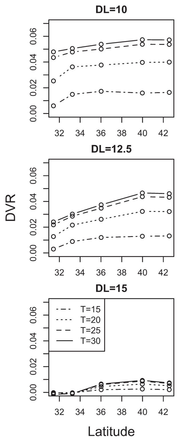
The relationship between the estimated developmental rate (DVR) and latitude as a function of temperature at 10 h, 12.5 h, 15 h day length. Circles represents estimated DVR and the cases at same temperature were connected with lines. In the plot, the horizontal axis shows the latitude at which each accession was collected. * the result of 30°C came from extrapolation.
Discussion
Model evaluation
As a result of quasi-R2 based on the PRESS for all five accessions, the nonlinear models were superior to the linear models (Table 4). In addition, the nonlinear models had the lowest values of Akaike’s information criterion (AIC; Akaike 1973). The difference between the quasi-R2 and AIC values for the nonlinear and linear models decreased with decreasing latitude. This result and sectional views in Fig. 2 demonstrated that photoperiod sensitivity had strong non-linearity in the accessions of Hokkaido and Akita, thus non-linear model was suited. In northern areas of Japan, suitable periods for wild soybean to flower would be shorter than in southern areas of Japan, therefore even in longer photoperiod season, these accessions need to prepare for flowering; as a result, DVR stayed high even in the conditions close to critical day length, and it caused the non-linearity. As the large estimated linear parameter shown in Table 3 indicates, DVR was almost proportional to day length in the case of accession of Miyazaki. Thus, the quasi-R2 based on PRESS and AIC of linear model and non-linear model shown in Table 4 were not quite different.
Evaluation of the model accuracy by comparing the observed flowering initiation with the simulated values
The results of simulations (described in Table 5) showed that corrected models predicted flowering initiation well in the case observed in original area for each accession. Residual days between predicted and observed date were just one day in the cases of Ibaraki and Miyazaki accessions planted in original area. Implementation of the correction with effective day length worked well to predict the flowering initiation at open air field.
The prediction of the flowering initiation for accession of Saga planted in Saga was not so good as others; it was too early than actual flowering initiation. The simulated DVR of Ibaraki and Saga before the summer solstice were higher than other cases, as is shown in Fig. 3. As we could see in sectional views of Fig. 2, the estimated DVR for accessions of Ibaraki and Saga (0.0248 and 0.0228, respectively) at the condition, T = 25 and DL = 14, were higher than observed DVR (0.0148 and 0.0143, respectively). In the period between late April and early May, the day length in Ibaraki and Saga are around 14 hours, then the overestimation for these periods would make predictions faster than actual cases. The relatively low accuracy in Saga accession might be affected by this overestimation.
The effects of shoot emergence date to flowering initiation date
Since our model assumed that counting of development index starts from immediately after shoot emergence, it is important to evaluate the effects of those timings. In our study, the number of days to shoot emergence at the condition of T = 15°C were clearly longer than other conditions, but did not vary greatly among accessions and day lengths (Table 2) because we scarified the seed surface before sowing. However, most accessions of wild soybean in Japan are known to exhibit seed dormancy (Shimamoto 1994), the shoot emergence date would vary more widely due to variations in precipitation, temperature, or various kinds of disturbance under natural conditions. Thus, the uncertainty in the models of predicting the shoot emergence would increase, and it must be hard to predict the variations in shoot emergence dates.
Given the difficulty in predicting the shoot emergence timing, how far the variations in shoot emergence timing affects the timing of flowering initiation. Our results suggest that the shoot emergence date did not correspond directly to flowering initiation date. In accessions of Hokkaido and Akita, despite the assumed shoot emergence dates are different for 2 months, the predicted flowering initiation timings were almost unchanged (2 days and 6 days, respectively). Considering that flowering duration of an individual of wild soybean last for about 1 month (Nakayama and Yamaguchi 2002), the large variation in the shoot emergence date within a population would not affect the whole flowering duration of the population so much in the northern population of wild soybean. On the one hand, the cases of accessions in the area south from Ibaraki would be otherwise, the predicted flowering initiation dates were delayed for 14–29 days with the 2 month delay of assumed shoot emergence dates. Considering this result, whole flowering duration of the population might be extended for nearly a month in those areas. It is necessary to consider the shoot emergence timing for risk assessment of gene flow from GM soybean, especially in the southern part of Japan. It will be useful in those area to survey the shoot emergence timing and its variances and to use the observed data for the prediction of flowering initiation.
Latitudinal cline
Under short-day conditions, there were no clear differences among accessions, except for a lower DVR for the Miyazaki accession (Fig. 4). This indicates that the Miyazaki accession required higher temperatures and longer growth period, even under short-day conditions. At longer photoperiods, the latitudinal cline became clearer (Fig. 4). For example, at DL = 12.5, clear cline of DVR were observed between Akita (39.98 °N) to Miyazaki (31.43 °N) regardless of temperature conditions. However, in some cases between relatively close areas, such as Hokkaido and Akita at all day length or Saga and Miyazaki at DL = 15, the relationship between latitudes and photoperiodic sensitivity were not proportional. It may be due to the relatively small genetic differentiation in those areas. In either way, a clear latitudinal cline of photoperiodic sensitivity was observed on the scale of Japan as a whole. This result suggests that the rough prediction of flowering initiation would be possible based on latitude.
In the case of cultivated soybean, four major loci, E1, E2, E3 and E4 are known to be associated in response to longer photoperiod conditions (Buzzell 1971, Buzzell and Voldeng 1980, Cober et al. 1996, Cober and Voldeng 2001, Saindon et al. 1989). It is known their loss-of-function causes earlier flowering initiation, and those traits were selected artificially to be adopted cultivated soybean to higher latitudes. For example, a loss-of-function single-nucleotide allele at locus E1 (e1-as), which regulates the suppression of flowering locus T, leads to earlier flowering (Xia et al. 2012). Tsubokura et al. (2014) examined the relationship between the genotypes at the E1–E4 loci and the flowering timing of 63 accessions covering several ecological types, and reported that 62–66% of variation of flowering timing were explained by allelic combinations of these genotypes.
Zhang et al. (2008) reported that the circadian rhythmic expression of the blue light receptor GmCRY1a protein correlates with photoperiodic flowering and latitudinal distribution of soybean cultivars. Ishibashi and Setoguchi (2012) examined the relationships between polymorphism in GmCRY1a and a latitudinal cline of wild soybean, then concluded that the polymorphism was not associated with photoperiodic flowering cline of wild soybean, and speculated that the balancing selection of GmCRY1a might be involved in the photoperiodic flowering of wild soybean along a latitudinal cline. The observed latitudinal cline in photoperiodic sensitivity of wild soybean in Japan may be associated with the allelic combinations in genotypes of E1–E4 loci or unidentified genes.
Future challenges
If we can predict the flowering duration of crops and wild relatives such as the case of GM soybean and wild soybean before the determination of sowing date or the variety of crops, the risk of introgression would be reduced by temporal isolation with adjusting sowing date of varieties.
Our research focused on the sensitivity of flowering initiation to photoperiod and temperature for wild soybean: we were able to obtain reliable nonlinear predictive models for flowering initiation. Prediction of the timings of flowering initiation of soybean and wild soybean is the first step for the predicting the whole flowering duration. However, it is also necessary to predict the flowering pattern (initiation, peak or flowering end) to evaluate the risk of outcrossing between soybean and wild soybean, because it would affect the degree of flowers of 2 species existing simultaneously.
Acknowledgments
This research was supported by our colleagues from the Experimental Farm Management Division of the National Institute for Agro-Environmental Sciences. We thank K. Abe, T. Ara, Y. Iizumi, H. Yamaguchi and K. Watanabe. The survey of flowering in open air fields was supported by H. Araki (Hokkaido University), H. Tsuyuzaki (Akita Prefectural University), S. Horimoto (ex-Saga University), A. Nishiwaki (Miyazaki University) and their staffs. We also thank G. Sakurai and T. Miwa (NIAES) for useful advice with statistical analysis and positive comments on the early versions of this manuscript. We thank anonymous reviewers for their useful and kindful comments to improve our manuscripts. This research was supported by the project, “Genomics for agricultural innovation”, from the Ministry of Agriculture, Forestry and Fisheries of Japan.
Literature Cited
- Akaike, H. (1973) Information theory and an extension of the maximum likelihood principle. In: Petrov, B.N. and Csaki F. (eds.) 2nd International Symposium on Information Theory, Akademiai Kiado, Budapest, pp. 267–281. [Google Scholar]
- Allen, D.M. (1974) The relationship between variable selection and data augmentation and a method for prediction. Technometrics 16: 125–127. [Google Scholar]
- Buzzell, R.I. (1971) Inheritance of a soybean flowering response to fluorescent-daylength conditions. Can. J. Genet. Cytol. 13: 703–707. [Google Scholar]
- Buzzell, R.I. and Voldeng, H.D. (1980) Inheritance of insensitivity to long daylength. Soyb. Genet. Newsl. 7: 26–29. [Google Scholar]
- Chiang, Y.C. and Kiang, Y.T. (1987) Geometric position of genotypes, honeybee foraging patterns and outcrossing in soybean. Bot. Bull. Acad. Sinica 8: 1–11. [Google Scholar]
- Cober, E.R., Tanner, J.W. and Voldeng, H.D. (1996) Genetic control of photoperiod response in early-maturing, near-isogenic soybean lines. Crop Sci. 36: 601–605. [Google Scholar]
- Cober, E.R. and Voldeng, H.D. (2001) A new soybean maturity and photoperiod-sensitivity locus linked to E1 and T. Crop Sci. 41: 698–701. [Google Scholar]
- De Wit, C.T., Bronwer, R. and Penning de Vries, F.W.T. (1970) The simulation of photosynthetic systems. Proc. of the IBP/P1, Technical Meeting, Trebon (1969, PUDOC), Wageningen, pp. 47–60. [Google Scholar]
- Ellizondo, D.A., McClendon, R.W. and Hoogenboom, G. (1994) Neural network models for predicting flowering and physiological maturity of soybean. Trans. ASAE 37: 981–988. [Google Scholar]
- Ellstrand, N.C., Prentice, H.C. and Hancock, J.F. (1999) Gene flow and introgression from domesticated plants into their wild relatives. Ann. Rev. Ecol. Syst. 30: 539–563. [Google Scholar]
- Fehr, W.R. and Caviness, C.E. (1977) Stages of Soybean Development. Cooperative Extension Service, Agriculture and Home Economics Experiment Station Iowa State University, Ames, Iowa. [Google Scholar]
- Golub, G. and Pereyra, V. (2003) Separable nonlinear least squares: the variable projection method and its applications. Inverse Probl. 19: 1–26. [Google Scholar]
- Horie, T. and Nakagawa, H. (1990) Modelling and prediction of developmental process in rice: I. Structure and method of parameter estimation of a model for simulating developmental process toward heading. Japan. Jour. Crop Sci. 59: 687–695. [Google Scholar]
- Hymowitz, T. and Newell, C.A. (1981) Taxonomy of the genus Glycine, domestication and uses of soybeans. Econ. Bot. 35: 272–288. [Google Scholar]
- Ishibashi, N. and Setoguchi, H. (2012) Polymorphism of DNA sequences of cryptochrome genes is not associated with the photoperiodic flowering of wild soybean along a latitudinal cline. J. Plant Res. 125: 483–488. [DOI] [PubMed] [Google Scholar]
- Kaga, A., Tomooka, N., Phuntsho, U., Kuroda, Y., Kobayashi, S., Isemura, T., Gilda, M.J. and Vaughen, D.A. (2005) Exploration and collection for hybrid derivatives between wild and cultivated soybean: preliminary survey in Akita and Hiroshima Prefectures, Japan. Ann. Rep. Exp. Intro. Plant Genet. Resour. 21: 59–71. [Google Scholar]
- Kuroda, Y., Kaga, A., Tomooka, N. and Vaughan, D.A. (2006) Population genetic structure of Japanese wild soybean (Glycine soja) based on microsatellite variation. Mol. Ecol. 15: 959–974. [DOI] [PubMed] [Google Scholar]
- Ma, F.S., Cholewa, E., Mohamed, T., Peterson, C.A. and Gijzen, M. (2004) Cracks in the Palosade cuticle of soybean seed coats correlate with their permeability to water. Ann. Bot. 94: 213–228. [DOI] [PMC free article] [PubMed] [Google Scholar]
- Masuda, M. and Washitani, I. (1990) A comparative ecology of the seasonal schedules for “Reproduction by Seeds” in a moist tall grassland community. Funct. Ecol. 4: 169–182. [Google Scholar]
- Nakayama, Y. and Yamaguchi, H. (2000) Life history of wild soybean on natural populations. J. Weed Sci. Tech. 39: 182–183. [Google Scholar]
- Nakayama, Y. and Yamaguchi, H. (2002) Natural hybridization in wild soybean (Glycine max ssp. soja) by pollen flow from cultivated soybean (Glycine max ssp. max) in a designed population. Weed Biol. Manag. 2: 25–30. [Google Scholar]
- Ohigashi, K., Mizuguti, A., Yoshimura, Y., Matsuo, K. and Miwa, T. (2014) A new method for evaluating flowering synchrony to support the temporal isolation of genetically modified crops from their wild relatives. J. Plant Res. 127: 109–117. [DOI] [PubMed] [Google Scholar]
- Piper, E.L., Boote, K.J., Jones, J.W. and Grimm, S.S. (1996) Comparison of two phenology models for predicting flowering and maturity date of soybean. Crop Sci. 36: 1606–1614. [Google Scholar]
- Saindon, G., Beversdorf, W.D. and Voldeng, H.D. (1989) Adjusting of the soybean phenology using the E4 loci. Crop Sci. 29: 1361–1365. [Google Scholar]
- Sakamoto, S. and Toriyama, K. (1967) Studies on the breeding of non-seasonal short duration rice varieties, with special reference to the heading characteristics of Japanese varietes. Phyton. 22: 177–185. [Google Scholar]
- Sameshima, R. (2000) Modeling soybean growth and development responses to environmental factors. Bull. National Agricultural Research Center 32: 1–119. [Google Scholar]
- Setiyono, T.D., Weiss, A., Specht, J., Bastidas, A.M., Cassman, K.G. and Dobermann, A. (2007) Understanding and modeling the effect of temperature and daylength on soybean phenology under high-yield conditions. Field Crop Res. 100: 257–271. [Google Scholar]
- Shimamoto, Y. (1994) Wild soybean distribute in Hokkaido—its ecology and genetic structure—. Bull. Tohoku University, Institutes of Genetic Ecology 25: 1–4. [Google Scholar]
- Thomas, B. and Vince-Prue, D. (1997) Photoperiodism in plants (Academic, New York: ). [Google Scholar]
- Tollenaar, M., Daynard, T.B. and Hunter, R.B. (1979) Effect of temperature on rate of leaf appearance and flowering date in maize. Crop Sci. 19: 363–366. [Google Scholar]
- Tsubokura, Y., Watanabe, S., Xia, Z.G., Kanamori, H., Yamagata, H., Kaga, A., Katayose, Y., Abe, J., Ishimoto, M. and Harada, K. (2014) Natural variation in the genes responsible for maturity loci E1, E2, E3 and E4 in soybean. Ann. Bot. 113: 429–441. [DOI] [PMC free article] [PubMed] [Google Scholar]
- Warrington, J. and Kanemasu, E.T. (1983) Corn growth response to temperature and photoperiod. 1. Seedling emergence, tassel initiation and anthesis. Agron. J. 75: 749–754. [Google Scholar]
- Wen, Z.L., Ding, Y., Zhao, T. and Gai, J. (2009) Genetic diversity and peculiarity of annual wild soybean (G. soja Sieb. et Zucc.) from various eco-regions in China. Theor. Appl. Genet. 119: 371–381. [DOI] [PubMed] [Google Scholar]
- Wilkerson, G.G., Jones, J.W., Boote, K.J., Ingrain, K.T. and Mishoe, J.W. (1983) Modeling soybean growth for management. Trans. ASAE 26: 63–73. [Google Scholar]
- Wilson, H.K. (1928) Wheat, soybean, and oat germination studies with particular reference to temperature relationships. Agron. J. 20: 599–619. [Google Scholar]
- Xia, Z.G., Watanabe, S., Yamada, T., Tsubokura, Y., Nakashima, H., Zhai, H., Anai, T., Sato, S., Yamazaki, T., Lü, S.X.et al. (2012) Positional cloning and characterization reveal the molecular basis for soybean maturity locus E1 that regulates photoperiodic flowering. Proc. Natl. Acad. Sci. USA 109: E2155–E2164. [DOI] [PMC free article] [PubMed] [Google Scholar]
- Zhang, Q.Z., Li, H.G., Li, R., Hu, R.B., Fan, C.M., Chen, F.L., Wang, Z.H., Liu, X., Fu, Y. and Lin, C.T. (2008) Association of the circadian rhythmic expression of GmCRY1a with a latitudinal cline in photoperiodic flowering of soybean. Proc. Natl. Acad. Sci. USA 105: 21028–21033. [DOI] [PMC free article] [PubMed] [Google Scholar]