Abstract
Brain activity is a dynamic combination of different sensory responses and thus brain activity/state is continuously changing over time. However, the brain’s dynamical functional states recognition at fast time-scales in task fMRI data have been rarely explored. In this work, we propose a novel 5-layer deep sparse recurrent neural network (DSRNN) model to accurately recognize the brain states across the whole scan session. Specifically, the DSRNN model includes an input layer, one fully-connected layer, two recurrent layers and a softmax output layer. The proposed framework has been tested on seven task fMRI datasets of Human Connectome Project. Extensive experiment results demonstrate that the proposed DSRNN model can accurately identify the brain’s state in different task fMRI datasets and significantly outperforms other auto-correlation methods or non-temporal approaches in dynamic brain state recognition accuracy. In general, the proposed DSRNN offers a new methodology for basic neuroscience and clinical research.
Index Terms: dynamic brain state, recurrent neural network, fMRI, brain networks
I. Introduction
UNDERSTANDING the nature of brain’s activities and functions has been one of the major goals since the inception of neuroscience. During the past few decades, researchers have developed various methods to characterize and analyze the brain activity patterns, such as GLM [1], ICA [2], and sparse representation based methods [3–7]. The underlying assumption used in previous studies is that the brain networks and activation patterns/states are temporally stationary across the entire fMRI scan session. However, there are accumulating evidences [8–12] indicating that brain activities and states are under dramatic temporal changes at various time scales. For instance, it has been found that each cortical brain area runs different “programs” according to the cognitive context and the current perceptual requirements [9], and the intrinsic cortical circuits mediate the moment-by-moment functional state changes in the brain [9]. That is, in the brain’s dynamic functional process, parts of the brain engage and disengage in time, allowing a person to perceive objects or scenes, and to separate remembered parts of an experience, and to bind them all together into a coherent whole [8, 13]. What’s more, it is still under dynamic changes even in resting state within time scales of seconds to minutes [14]. Inspired by these observations, more and more researchers are motivated to examine the temporal dynamics of functional brain activities [15–19].
Currently, a dominant analysis technique used for describing the temporal dynamics of functional brain activities is the use of sliding windows [16, 20, 21]. Sliding window based approaches pre-specify the temporal resolution of the changing pattern (window size), and map the spatial distribution of the networks and provide measures of dependence, e.g., linear correlation between the timecourse for interested pair of voxels, regions, or networks [22]. These methods range from windowed versions of standard seed-based correlation or independent component analysis (ICA) techniques to new methods that consider information from individual time points [14, 16, 19–21, 23–27]. In addition to sliding window approaches, researchers also tried some alternative methods over the past few years. For instance, change point detection methods have been proposed to determine “brain state” changes based on the properties of data-driven partitioned resting state fMRI (rs–fMRI) data, such as amplitude and covariance of time series [10, 15, 18, 28–31]. In contrast to methods based on relationships between brain regions, event-based approaches assume that the brain activity is primarily composed of distinct events and these events can be deciphered from the BOLD fluctuations [32, 33] or through deconvolution of a given hemodynamic model from the time series [34, 35]. More recently, Vidaurre and his colleagues proposed to describe brain activity as a dynamic sequence of discrete brain states using Hidden Markov Model (HMM) to provide a rich description of the brain activities [36, 37]. In general, these approaches have enriched the description of functional brain activities and contributed to the better understanding of the temporal dynamics underlying brain activities.
However, these approaches might still have possible limitations. First, as the most widely used approach, the parameters of sliding window techniques are debatable, such as the window length and type. For example, a long temporal).window will miss fast dynamics, while short window will have insufficient data to provide reliable estimation, and it is difficult to achieve convincible results without “gold standard”. Second, most of these approaches make conclusions based on the relative changes between paired voxels or brain regions which ignore the temporal dependence of the whole sequence of brain activities/states. In addition, with the limited time scales, they may not be able to catch the fast temporal scale dynamics. Last but not least, many of these methods are designed for rs-fMRI data [22] and how to model the temporal dynamics of task fMRI (tfMRI) data has been rarely explored. Therefore, developing a comprehensive and systematic spatial-temporal brain dynamic activity modelling framework that can naturally recognize dynamic brain states at fast time-scales from task fMRI data is still needed.
Recently, Recurrent Neural Networks (RNNs) have shown particularly outstanding performances in many research areas, such as handwriting recognition [38, 39], language modeling [38,40], machine translation [41], and speech recognition [42], which involve modeling sequential signals. Furthermore, a few attempts using RNNs in neural encoding [42] and responding [48] have shown that RNNs are feasible in modeling dynamic biological signals. A prominent feature of RNNs is that they can easily and effectively capture both short and long term temporal dependences in data sequences and model the inner dependent relationships using their internal memories. Specifically, RNNs maintain memory cells to preserve the information of the past sequences and learn when and how to restore these memories to make predictions, rather than predicting based only on local neighborhoods in time. Therefore, RNNs can inherently acquire the temporal dependence of the sequential data, which is quite suitable for the problem of modeling temporal dynamic activities and recognizing the fast time-scale brain states in task fMRI data.
Inspired by the great ability in modeling the temporal dependence of sequential data using RNN models, in this paper, we propose a five-layer deep sparse recurrent neural network (DSRNN) to recognize the dynamical brain states at fast time-scales in tfMRI data. Briefly, the proposed DSRNN model includes an input layer, one fully-connected layer, two recurrent layers and a softmax output layer. We tested the proposed DSRNN model with more than 800 subjects in the seven task fMRI datasets provided by the Human Connectome Project (HCP), including working memory, gambling, motor, language, social, relational, and emotion tasks [49]. Notably, the proposed DSRNN model achieved outstanding brain state recognition accuracy (over 90 percent averagely), compared with auto-correlation methods (Adaptive Autoregressive Classifier, AAR [50, 51]) and traditional non-temporal modeling approaches (Softmax and SVM). Also, the associated important brain regions in recognized brain states show meaningful consistence with traditional task-activated areas, which provides us novel insight on understanding the brain activities and functions. In general, our work demonstrate that the proposed DSRNN model has great advantage in recognizing the dynamical brain states at fast time-scales, and it offers a novel methodology for the study of dynamical functional brain activities.
II. Materials and Methods
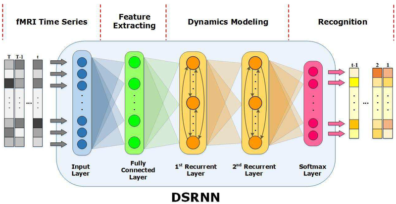
The proposed deep sparse recurrent neural network (DSRNN) is a five-layer deep neural network model, including an input layer, one fully-connected layer, two recurrent layers and a softmax output layer. Specially, the fully-connected layer plays a role of extracting activated brain regions and reducing data dimension, and the cascaded recurrent layers are used to capture temporal dependence in time series. In this section, we will introduce the fMRI datasets, basic theory of recurrent neural network, and the structure and mechanism of DSRNN in details.
A. Data Acquisition and Pre-processing
In this paper, we adopted the Human Connectome Project (HCP) 900 Subjects Data Release as test beds, which include behavioral and 3T MR imaging data for over 900 healthy adult participants [52]. Seven categories of behavioral tasks are involved, including Working memory, Gambling, Motor, Language, Social, Relational, Emotion tasks. The design information of seven tasks is shown in Table 1. In total, there are 788 subjects executed all seven behavioral tasks, and 786 subjects’ task fMRI (tfMRI) time series with good data quality are used in this work. All the datasets are available on https://db.humanconnectome.org. The detailed acquisition parameters were set as follows: 220 mm FOV, inplane FOV: 208×180 mm2, flipangle=52, BW=2290 Hz/Px, 2 × 2 × 2 mm3 spatial resolution, 90×104 matrix, 72 slices, TR=0.72s, TE=33.1ms. The preprocessing of these tfMRI data sets includes skull removal, motion correction, slice time correction, spatial smoothing, and global drift removal (high-pass filtering). In our implementation, a 4 × 4 × 4 mm3 downsampling is applied to reduce computational cost. Next, we will introduce these tasks briefly and more detailed procedures are available in section A of supplementary materials. Supplementary materials are available in the supplementary files /multimedia tab.
TABLE I.
Properties of HCP task-fMRI datasets
| Parameters╲Task | Working Memory | Gambling | Motor | Language | Social | Relational | Emotion |
|---|---|---|---|---|---|---|---|
| # of Frames | 405 | 253 | 284 | 316 | 274 | 232 | 176 |
| Duration (Min) | 5:01 | 3:12 | 3:34 | 3:57 | 3:27 | 2:56 | 2:16 |
| # of Task Blocks | 8 | 4 | 10 | 8 | 5 | 6 | 6 |
| # of Block Labels | 3 | 3 | 6 | 3 | 5 | 3 | 3 |
| Duration of Blocks(s) | 25 | 28 | 12 | See Text | 23 | 16 | 18 |
In working memory (WM) task, a version of the N-back task was used to assess working memory [53]. It was reported that the associated brain activations were reliable across subjects [53] and time [54]. Gambling task was adapted from Delgado et al. [55], and prior works demonstrated that the task elicits activations in the striatum and other reward related regions which are robust and reliable across the subjects [55–58]. Motor task was developed by Buckner and his colleagues which has been proven that it could identify effector specific activations in individual subjects [59]. Language task was developed by Binder et al. [60]. There are two subtasks: story and math where the math blocks was designed to provide a comparison task that was attentional demanding. In Social task, an engaging and validated video task was chosen as a measure of social cognition, giving evidence that it generates robust task related activation in brain regions associated with social cognition and it is reliable across subjects [61–64]. Relational task was adapted from the one developed by Smith et al. [65] which demonstrated to localize activation in anterior prefrontal cortex in individual subjects. Emotion task was adapted from Hariri and his colleagues who have shown this task could be used as a functional localizer [66] with moderate reliability across time [67].
B. Recurrent Neural Networks
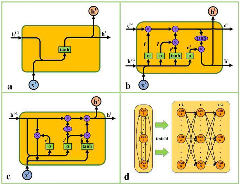
Recurrent neural networks (RNNs) are feedforward neural networks with edges connecting adjacent time steps. This distinct architecture is similar to biological neuronal networks, where lateral and feedback interconnections are widespread. The internal states of RNNs preserve memories of previous state information and capture the temporal dependences of input signals. RNNs have been applied successfully in many diverse sequence modeling tasks [38–48, 68]. Fig. 1(a) illustrates a specific and basic recurrent cell unit and its recursive equation is as follows:
| (1) |
where U , W are the weight matrices for hidden states and input features and b is bias parameters. ht denotes the hidden state. Typically, vanilla RNNs (established by basic recurrent cell units) are very dificult to train due to the vanishing gradient problem [69]. In contrast, LSTM (Long Short-Term Memory) units [70] and GRU (Gated Recurrent Unit) units [41] were specifically designed to overcome this problem and have since become the most widely-used cell architectures.
Fig. 1.
A schematic illustration of RNN cell models. (a) The nonlinear basic recurrent cell unit; (b) Long short-term memory unit; (c) Gated recurrent unit; (d) The interconnections in a common recurrent hidden layer. Neurons in recurrent layer are fully interconnected and new hidden states can be influenced by all former states. Squares indicate linear combination and nonlinearity. Circles indicate element wise operations. Gates in the units control the information flow between adjacent time points.
Each LSTM unit maintains a cell state that acts as its internal memory by storing information from previous time series. The contents of the cell state are controlled by the gates of the unit, and determine unit’s hidden state. The first–layer hidden state of an LSTM unit is defined as follows:
| (2) |
| (3) |
where ⊙ denotes elementwise multiplication, ct is the cell state, and ot is the output gate activation. The output gate controls what information would be retrieved from the cell state. The cell state of an LSTM unit is defined as:
| (4) |
| (5) |
| (6) |
| (7) |
where ft is the forget gate activation, it is the input gate activation, and is an auxiliary variable. Forget gate controls what old information would be abandoned from the cell state, while input gate controls what new information would be stored in cell state. Furthermore, U f, U i, U c and W f, W i, W c are the corresponding weights and b f, bi, bc are the biases (i.e., the learnable parameters of the model).
The GRU unit is a simpler alternative to LSTM unit. They combine hidden state with cell state, and input gate with forget gate. The first-layer hidden state of GRU unit is defined as follows:
| (8) |
| (9) |
| (10) |
| (11) |
where zt is update gate activation, rt is reset gate activation, and is an auxiliary variable. Like the gates in LSTM unit, those in GRU unit also control the information flow. As LSTM, trainable parameters, such as weights U z, U r , U h and W z, Wr, W h, and biases b z, b r, b h, determine the activations of the gates.
As shown in Fig. 1(d), a recurrent neural network can be unfolded as a deep feedforward network along time. Conversely, when the numbers of units and connections are limited, a desirable function computed by a very large feedforward network might alternatively be approximated by recurrent computations in a smaller network. Recurrent network can expand computational power by multiplying the limited physical resources for computation along time.
C. Deep Sparse Recurrent Neural Network
As described beforehand, the feedforward sweep alone might not provide the sufficient evidences that the output layer needs to confidently recognize brain states. Instead, an ideal model should integrate later-arriving lateral and top-down signals to converge on its ultimate response. Therefore, in order to better capture the temporal dependences preserved in fMRI time series and recognize the dynamical brain states, a five-layer DSRNN model is proposed, as shown in Fig 2. Adjacent layers are fully connected, and the connections between layers are forward. The fully connected layer plays a role as a filter of activated brain regions, which aims to winnow and combine significant fMRI volumes with proper weight values. Then, two recurrent layers are employed following the same structure, as shown in Fig.2, so that various scales of temporal dependences can be captured. The hidden state of second recurrent layer is defined similarly to that of first recurrent layer, except for replacing the input with the hidden state of first layer. Finally, we apply a softmax layer to obtain a vector of class probabilities:
| (12) |
| (13) |
where softmax .
Fig. 2.
Overview of the DSRNN model. The stretched fMRI vector sequences are fed to the input layer of DSRNN model. One fully connected layer is used to extract activated brain regions. Two recurrent layers with dropout are cascaded to model temporal dynamics. Finally, a softmax classifier is arranged for the brain state recognition.
In the training process of DSRNN, the optimization objective is made up of three components shown as follows:
| (14) |
The first term is the overall error cost. In the case of multiclass classification, the error cost is defined as the cross entropy (CE) between the true labels {y} and the predicted labels . The cross entropy for the discrete distributions P and Q over a given set is defined as follows:
| 15 |
The second term is the sparseness penalty of the activation (output) OFull of fully connected layer, and L1 norm helps to concentrate task related volumes in only a few patterns. β controls the weight of sparseness penalty term.
The last term is also a sparseness penalty which forces WFull to be sparse. WFull is the weight matrix of fully-connected layer. We use L1 norm as the penalty cost, and λ is the weight parameter of this penalty term. Because activated brain regions are extracted from WFull proper sparseness of WFull can help to remove those brain areas which are not sensitive to task events and to make significantly activated brain regions stand out.
DSRNN adopts the feedforward sweep to extract elementary features, and then uses subsequent recurrent computations to explain the nonlinear interactions of these features. In such a process, the information maintained in fMRI signals would be gradually uncluttered in the low-level representation and contextualized by the high-level representation. Therefore, the higher level brain states are recognized accurately and brain dynamics are modeled gradually.
The recognition accuracy is defined as the proportion of correctly recognized labels, and the calculation is as follows:
| 16 |
where LabelsRec are the recognized label sequences, and LabelsGT are the ground truth labels. Therefore, numerator is the number of time points which are correctly recognized.
In this paper, the DSRNN model is implemented with Ten-sorflow. Truncated back propagation through time is employed in conjunction with AdamOptimizer to train the models by iteratively minimizing the objective function (Equation (14)). Besides, dropout operation [71] was applied on the inputs of each recurrent layer, which enhances the generalization of DSRNN model. The DSRNN model was run on the computing platform with two GPUs (Nvidia GTX 1080 Ti, 12G Graphic Memory) and 64 G memory.
D. Random Fragment Strategy
In this paper, the datasets we used are from the Human Connectome Project (HCP) 900 Subjects Data Release. In HCP, all subjects followed the same task designs, and the recorded event label sequences were almost the same. However, if the whole fMRI series and event label sequences were used for training, it would cause a severe overfitting problem, that is, the DSRNN would only learn the task designs, rather than the temporal dependences hidden in fMRI time series, and the training process would be meaningless.
In order to overcome this drawback of datasets, we propose a novel training strategy: random fragment strategy (RFS). In this strategy, sequence fragment with random length is cut from random location of the sequence. Thus, in each iteration, new different sequence fragments are fed to DSRNN. In this paper, the fragment length ranges from 30%~50% of the whole sequence length. By creating huge amounts of distinct sequences with different lengths, RFS enriches the diversity of datasets and makes sure that the DSRNN learns the temporal dependences preserved in fMRI time series, rather than changeless arrangement of task events.
III. Results
A. Overview of the DSRNN Model
In order to validate the proposed DSRNN framework, we tested the DSRNN model on the Human Connectome Project (HCP) 900 Subjects Data release. Specifically, there are seven task fMRI datasets with more than 800 subjects which is one of the biggest publicly available tfMRI dataset. In the following sections, we will first go over the details of the DSRNN model and then discuss the brain state recognition results and associated important brain areas and the effects of different parameter settings. For convenience, we take motor task as an example, which includes the maximum stimulus events in HCP data sets.
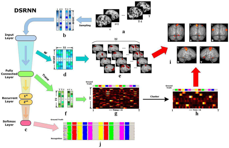
As shown in Fig. 3(a)~3(b), the 3-D whole brain fMRI recordings of time t , where brain state is hidden, are sent to the input layer of DSRNN after being stretched into a 1–D (28549∗1) vector. Then, the fully connected layer extracts activated brain regions, and converts the original large dimension (28549) recordings into small size (32) activations. Specially, activated brain regions are gradually filtered during the whole training process, and represented by the weights of fully connected layer, as shown in Fig. 3(d) ~ 3(e). As determined beforehand, we arranged 32 neuron units in fully connected layer, therefore, we obtained 32 groups of activated brain regions. After all the trainable parameters of DSRNN are settled, the activated brain regions are confirmed. In Fig. 3(e), it is easy to observe that there are a few specific brain areas activated in each group. In general, original recordings contain raw brain information, and they are definitely redundant. After this filtering process of fully connected layer, only those significant and distinctive information are preserved, and the redundancy is reduced largely (from 28,549 to 32). Therefore, the brain state corresponding to each task event can be indicated by only a few activated brain region groups. The activations of these region groups make up the outputs of fully connected layer, as shown in Fig. 3(f), where the vector size is much smaller than those in Fig. 3(b).
Fig. 3.
Illustration of DSRNN modeling process. (a) Raw brain tfMRI images series. (b) Vectorization of tfMRI image series after sampling. (c) Hierarchy diagram of DSRNN model. (d) Weight matrix between input layer and fully connected layer. (e) Visualization of activated brain region groups represented by weight matrix of fully connected layer. (f) Output time series of fully connected layer. Each column vector indicates the activation of 32 distinctive brain region groups. (g) Visualization of fully time-scale output time series of fully connected layer, also the activation traces of 32 brain region groups. Motor task is used as an example, and the ground-truth temporal distribution of event blocks is illustrated at the top. (h) Visualization of clustered activation traces.(i) Visualization of brain activation maps corresponding to 5 motions, based on 32 brain region groups (e) and their clustered activation traces (h). Brain activation maps from I to VI are corresponding to the motion events of right foot, left foot, tongue, left hand and right hand, respectively. (j) Recognition of brain states.
After assembling the output vectors (Fig. 3(f)) along time, we can obtain an activation trace map, as shown in Fig. 3(g), where the brain state shift can be illustrated more clearly. In this paper, we regard task design as ground truth since different task stimulus events are presented to the participants according to the task design paradigm. Comparing activation traces with the ground truth at the top of Fig. 3(g), it is easy to recognize matching relations between them. In addition, some activated region groups have similar shapes in activation trace, which indicates that these groups of regions may be activated simultaneously and they functionally cooperate with each other. Then, we further cluster all the region groups into several classes based on their activation traces, and the clustered trace map is shown in Fig. 3(h). In motor task, there are five different motion events: left foot, right foot, left hand, right hand, tongue. In Fig. 3(h), it is easy to observe that there are 5 clustered activation traces matching 5 motion events closely. We pick up the brain activation map corresponding to each motion, and show them in Fig. 3(i). In this way, the whole brain activation maps of each task event are obtained.
In addition, the activation traces are fed to recurrent layers to capture temporal dependences, which is vitally important to model dynamic system. With the outputs of the 2nd recurrent layer, softmax classifier can make an accurate recognition of brain states, as shown in Fig. 3(j).
B. Brain State Recognition via DSRNN
In this paper, we adopted HCP 900 Subjects data release as testbeds, including 786 subjects with good data quality, which guarantees the diversity and universality of the experiment. Although a 4 × 4 × 4 mm3 down-sampling is applied to reduce training data size, we still cannot put all subjects’ data in our computing platform’s memory (64G Memory, 24G Graphic Memory in total). Thus, we have to randomly pick up as many subjects as memory can hold. The quantity of training and testing subjects of each task is shown in Table 2.
TABLE II.
Training and testing subject numbers of seven tasks.
| Task | Train | Test |
|---|---|---|
| WM | 240 | 240 |
| GAMBLING | 320 | 320 |
| MOTOR | 320 | 320 |
| LANGUAGE | 300 | 300 |
| SOCIAL | 320 | 320 |
| RELATIONAL | 320 | 320 |
| EMOTION | 400 | 360 |
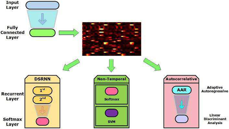
In Fig. 3(f) ~ 3(g), activation traces are obtained from fully connected layer, before where all processes have no relationships with temporal dependences processing. Since the human brain is a deep and complicated neural network[44], in which feedforward, lateral, and feedback connections are widespread, we suppose that there must be recurrent information flow of dynamics hidden in the fMRI time series. This is also the reason why we employed recurrent layers in DSRNN model. To validate this supposition, we compared the recurrent classifier (DSRNN model) with an auto correlative classifier (Adaptive Autoregressive Classifier, AAR) and two non-temporal classifiers (Softmax and SVM) respectively, as shown in Fig. 4.
Fig. 4.
Brain states recognition with recurrent layers, Softmax, SVM and AAR based on activation traces.
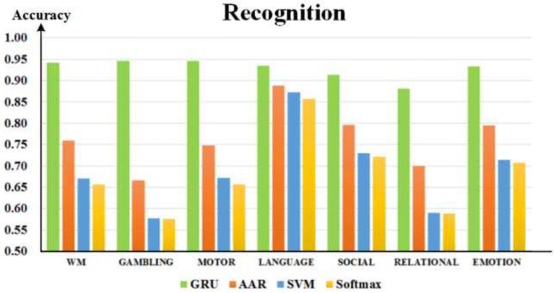
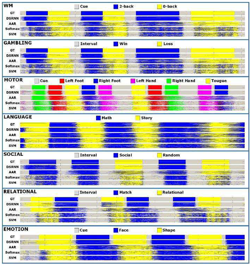
After training hundreds of subjects, DSRNN model achieved outstanding performance in test datasets, and the results are illustrated in Fig.5 and Fig. 6. From Fig. 5, it is easy to appreciate that DSRNN model recognized brain states of seven tasks with the highest accuracies (above 90%, except relational task 88%). The rank of recognition accuracy from high to low is: DSRNN > AAR > Softmax ≈SVM. Fig. 6 illustrates the recognized brain states using different methods across all subjects. It is easy to observe from Fig. 6 that DSRNN model detected every subtask block in each task accurately. It accurately recognized not only the task durations, but also the change points of states. In DSRNN’s series, event blocks are very clear, even for the “Interval/Cue” blocks. In contrast with DSRNN, auto-correlation classifier (AAR) and non-temporal classifiers (Softmax and SVM) perform much worse at the state change points, and there are also plenty of noises which make event blocks ambiguous. Besides, DSRNN’s recognition of the first event block in each task is not so accurate, compared with other blocks behind. This is quite reasonable, because DSRNN needs some input sequences to initially build its preservation of memory.
Fig. 5.
Brain state recognition accuracies of seven tasks.
Fig. 6.
Brain state series of seven tasks. In each subgraph, five state series from top to bottom are ground truth (GT), and series recognized by DSRNN,AAR, Softmax and SVM, respectively.
Before maintaining enough temporal information of previous series, the recognition cannot reach the best performance. This result further indicates the importance of temporal dependences in brain state recognition.
To conclude, our works demonstrated that DSRNN has better performance in brain state recognition than other models, especially those non-temporal classifiers.
C. Brain Activation Maps
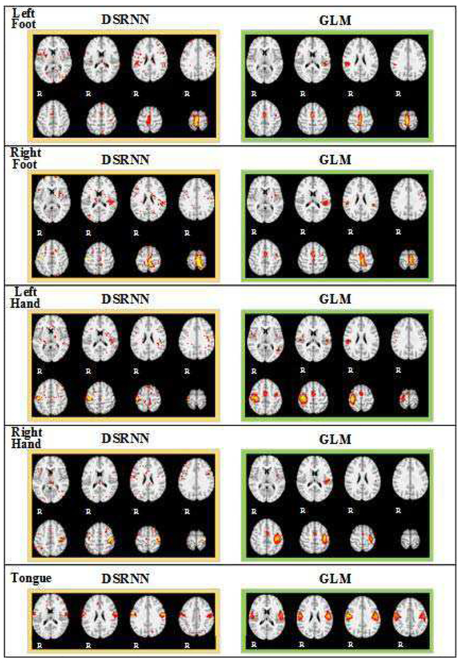
An important characteristic of the proposed DSRNN model is that we can also obtain the important activated brain areas involved in brain state recognition. During brain state recognition, distinctive activated brain regions for each task event were extracted (illustrated in Fig. 3(i)). In this paper, we applied DSRNN model on seven HCP tasks, therefore, seven groups of brain activation maps of each task were obtained. In order to interpret these associated brain areas involved in brain state recognition, we compared these spatial maps with the activation maps obtained by GLM method, we find that interesting correspondence between these maps. For convenience, we also take motor task as an example and put other task’s result into the section B of supplementary materials. Supplementary materials are available in the supplementary files /multimedia tab.
The activation maps for the motor task are shown in Fig. 7. Events of Left foot and right foot show great activations in the posterior portion of the frontal lobe. For left hand and right hand, besides these distinctions, activations in precentral cortex are very clear. In addition, bilateral precentral cortex are activated during tongue movement. In motor task, we can see clear spatial differentiation of the activations in motor cortex: left and right hand/foot motion have expected contralateral activation locations, whereas tongue motion activates bilateral regions.
Fig. 7.
Activation maps of motor task.
D. Effects of hyper parameters in DSRNN
In DSRNN, there are a few hyper parameters, such as cell unit number of each layer, recurrent layer number, and recurrent cell unit type, which determine the performance of DSRNN. Therefore, before the experiment, we need to determine all these hyper parameters carefully. In this paper, we picked up 100 subjects from working memory task datasets as test samples. By five-fold cross validation (80 subjects for training and 20 for test in each trial), we explored the effects on DSRNN’s recognition performance of each hyper parameter, and the exploration results are shown in Fig. 8 and Fig. 9.
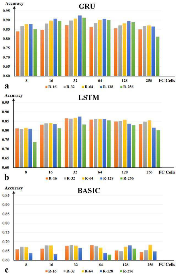
Fig. 8.
The exploration results of hyper parameters. (a) Results of GRUbased network. (b) Results of LSTM-based network. (c) Results of basic unitbased network. The horizontal axis represents the number of neurons in fully connected layer, and the vertical axis indicates the recognition accuracy. All networks contain two recurrent layers, and bars in different colors indicate different numbers of cell units per recurrent layer.
Fig. 9.
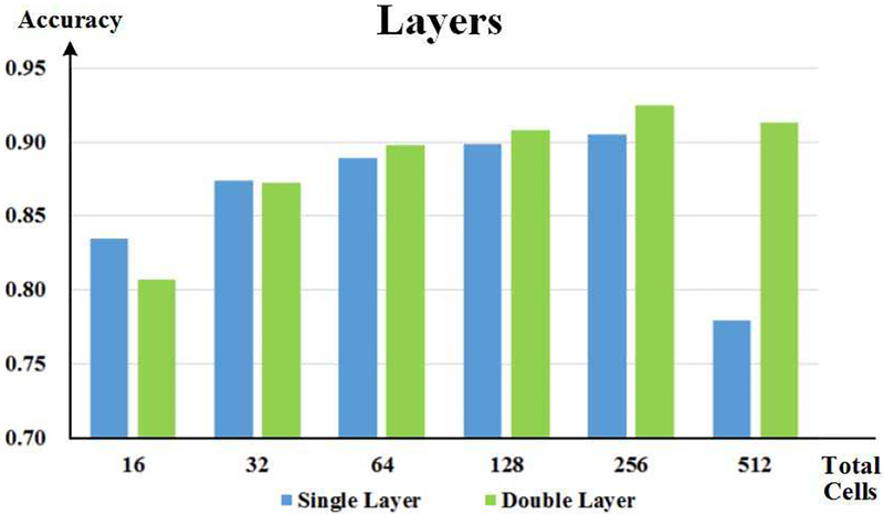
The exploration results of DSRNN with different numbers of recurrent layers. The horizontal axis represents the total number of recurrent cell units, and the vertical axis indicates the recognition accuracy. Bars in different colors indicate different recurrent layer numbers.
According to previous RNN studies [48], two recurrent layers might capture multi-scale temporal dependences in series, and they outperformed the network with only single recurrent layer. So in the exploration of hyper parameters, we assumed that DSRNN with two recurrent layers might perform better than only one layer. Based on this assumption, we explored the effects of three hyper parameters: the cell number of fully connected layer, the cell unit number of each recurrent layer, and the cell type of recurrent layer. In Fig. 8(a), with GRU unit being the recurrent cell, DSRNN reached the highest performance when fully connected layer cell number was 32, and 128 GRU units were in each recurrent layer. Then, we repeated the experiment with LSTM unit and basic cell unit, and the results are shown in Fig. 8(b) and Fig. 8(c). In Fig. 8(b), network with 32 cells in fully connected layer and 128 LSTM units in each recurrent layer also performed slightly better than others. Compared with the results of GRU units, LSTM units achieved lower recognition accuracy by about 5%, on average. As to basic recurrent unit, the accuracy of recognition was even worse, which was less than 70%, and some were even below 60%. Therefore, after comparing the performances of different combinations of three hyper parameters (the cell number of fully connected layer, the cell unit number of each recurrent layer, and the cell type of recurrent layer), we determined the architecture of DSRNN, which included a 32–cell fully connected layer, and two 128-GRU-based recurrent layers.
As all other hyper parameters were confirmed, we explored the influences of different recurrent layer numbers on DSRNN’s performances. In order to make a comparison, we made sure that both architectures had the same number of recurrent cell units (GRU), so that the performance would be only determined by the cell arrangement. The results are shown in Fig. 9. When there were only a small number of recurrent units, all units arranging in parallel in one layer achieved better recognition accuracy than cascaded arrangement. With the increase of cell number, the accuracies of both architectures improved, and the two-layer improved more. With a total of 256 recurrent cell units, both architectures reached the top, and two-layer architecture performed better. This result demonstrated that with sufficient cell units, arrangement of two cascaded recurrent layers could capture time dependences better than using only single layer arrangement.
E. Effects of free parameters in DSRNN
Based on the optimal structure of DSRNN, the free parameters of DSRNN, which should be determined before formal experiments, can be explored. In this paper, there are three free parameters that we needed to focus on: two sparseness penalty weights β and λ, and keeping proportion of dropout.
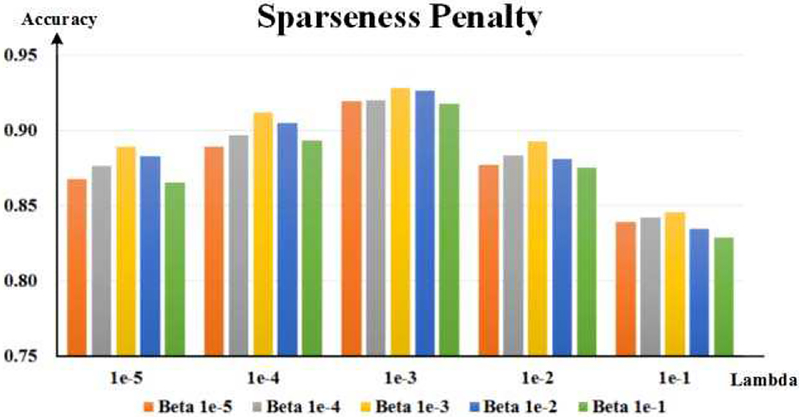
To investigate β and λ, we tried orders of magnitude ranging from 1e–6 to 1e–1. The recognition results of different combinations of β and λ are shown in Fig. 10. It is easy to see that λ has greater influences on DSRNN model than β, while β provides fine-tuning to DSRNN’s performance. When β and λ both were set 1e–3, DSRNN model achieved the best performance.
Fig. 10.
The exploration results of sparseness penalty weights: beta and lambda. The horizontal axis indicates the values of lambda, and the vertical axis denotes the recognition accuracy. Bars in different colors indicate different beta values.
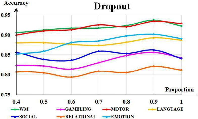
Dropout operation is also introduced to enhance the generalization of DSRNN model. As all other parameters are decided, it is feasible to select the best proportion based on all seven tasks. We tried the proportion from 0.4 to 1.0, and found that DSRNN performed the best at 0.9. It can be inferred that there is high consistency among subjects in each task, and DSRNN can model fast time-scale brain states effectively and robustly.
IV. Discussion and Conclusion
In this paper, a 5–layer deep sparse recurrent neural network (DSRNN) model is proposed to model the dynamic brain states in task fMRI data. With outstanding capability of capturing sequence temporal dependence, DSRNN can recognizes brain states accurately. In addition, the associated brain activated regions also demonstrate meaningful correspondence with traditional GLM activation results which provide us novel insight on functional brain activities. Comparing with common auto-correlation modeling method (AAR) and traditional nontemporal modeling approaches (Softmax and SVM), DSRNN achieved obviously outstanding recognition accuracy.
Though current DSRNN model has achieved excellent performances in brain states recognition accuracy, it still can be developed in a few aspects. Firstly, although the fully connected layer applied in DSRNN extracted distinctive activated brain regions successfully, there are many other neural network structures, such as CNN, DBN, etc., to be further revisited. These models are also widely used in computer vision and feature extraction, and have more complicated structure than fully connected layer. Better performance might be achieved if these models are employed. Secondly, in this paper, we recognize the brain states of each single task and obtained seven different state recognition models. Each model can identify subtasks or brain states of only one category of task. In the future, we can train one DSRNN model with all seven tasks. In this way, more distinctive activation maps and more differences can be obtained among tasks. Thirdly, as a proposal, DSRNN model might be applied online in the future. Because once the DSRNN model is trained successfully, real-time tfMRI data time seies can be fed online and the brain behaviors can be detected in quite a short time. This application can be used widely as a brain states identifier.
Finally, there are several potential applications in basic neuroscience and clinical research with the proposed DSRNN model. For instance, it has been observed that dynamic performance can be sensitive to psychiatric or neurologic disorders, and the associated brain areas in brain state recognition may provide novel insight for clinical diagnosis. Besides, many literatures suggest that the brain activities and states are under dynamical changes and the proposed model provide a useful tool to recognize the brain states at fast time-scale in task fMRI data. In general, our proposed DSRNN model offers a new methodology for basic and clinical neuroscience research.
Supplementary Material
Fig. 11.
The exploration of dropout proportion based on seven tasks. The horizontal axis indicates the proportion, and the vertical axis denotes the recognition accuracy. Curves in different colors indicate different tasks.
Acknowledgments
This work is supported by National Key R&D Program of China under contract No. 2017YFB1002201 and the Fundamental Research Funds for the Central Universities. H Wang was supported by the Fundamental Research Funds for the Central Universities, the National Natural Science Foundation of China (Grant No. 31627802). T. Liu is supported by NIH R01 DA–033393, NIH R01 AG–042599, NSF CAREER Award IIS–1149260, NSF BME-1302089, NSF BCS–1439051 and NSF DBI–1564736. S. Zhao was supported by the National Science Foundation of China under Grant 61806167, the Fundamental Research Funds for the Central Universities under grant 3102017zy030 and the China Postdoctoral Science Foundation under grant 2017 M613206. Li Xie was supported by the Zhejiang Province Science and Technology Planning Project No.2016C33069.
Contributor Information
Han Wang, College of Bio-medical Engineering & Instrument Science, Zhejiang University, 310027, Hangzhou, P. R. China..
Shijie Zhao, School of Automation, Northwestern Polytechnical University, Xi’an, 710072, China..
Qinglin Dong, Cortical Architecture Imaging and Discovery Lab, Department of Computer Science and Bioimaging Research Center, The University of Georgia, Athens, GA, 30602 USA..
Yan Cui, College of Bio-medical Engineering & Instrument Science, Zhejiang University, 310027, Hangzhou, P. R. China..
Yaowu Chen, College of Bio-medical Engineering & Instrument Science, Zhejiang University, 310027, Hangzhou, P. R. China..
Junwei Han, School of Automation, Northwestern Polytechnical University, Xi’an, 710072, China..
Li Xie, College of Bio-medical Engineering & Instrument Science, Zhejiang University, 310027, Hangzhou, P. R. China..
Tianming Liu, Cortical Architecture Imaging and Discovery Lab, Department of Computer Science and Bioimaging Research Center, The University of Georgia, Athens, GA, 30602 USA (corresponding author; phone: (706) 542-3478; tianming.liu@gmail.com).
References
- [1].Friston KJ, Holmes AP, Worsley KJ, Poline JP, Frith CD, and Frackowiak RSJ, Statistical parametric maps in functional imaging: A general linear approach, HUM BRAIN MAPP, vol. 2, (no. 4), pp. 189–210, 1994. [Google Scholar]
- [2].Mckeown MJ, Jung TP, Makeig S, Brown G, Kindermann SS, Lee TW, and Sejnowski TJ, Spatially independent activity patterns in functional MRI data during the stroop color-naming task, P NATL ACAD SCI USA, vol. 95, (no. 3), pp. 803–810, 1998. [DOI] [PMC free article] [PubMed] [Google Scholar]
- [3].Lv J, Jiang X, Li X, Zhu D, Chen H, Zhang T, Zhang S, Hu X, Han J, and Huang H, Sparse Representation of Whole-brain FMRI Signals for Identification of Functional Networks, MED IMAGE ANAL, vol. 20, (no. 1), pp. 112–134, 2014. [DOI] [PubMed] [Google Scholar]
- [4].Zhao S, Han J, Lv J, Jiang X, Hu X, Zhao Y, Ge B, Guo L, and Liu T, Supervised Dictionary Learning for Inferring Concurrent Brain Networks., IEEET MED IMAGING, vol. 34, (no. 10), pp. 2036, 2015. [DOI] [PubMed] [Google Scholar]
- [5].Jiang X, Zhao L, Liu H, Guo L, Kendrick KM, and Liu T, A Cortical Folding Pattern-Guided Model of Intrinsic Functional Brain Networks in Emotion Processing, FRONT NEUROSCI-SWITZ, vol. 12, 2018–08–21 2018. [DOI] [PMC free article] [PubMed] [Google Scholar]
- [6].Lv J, Jiang X, Li X, Zhu D, Zhang S, Zhao S, Chen H, Zhang T, Hu X, and Han J, Holistic atlases of functional networks and interactions reveal reciprocal organizational architecture of cortical function, IEEE T BIO-MED ENG, vol. 62, (no. 4), pp. 1120–1131, 2015. [DOI] [PubMed] [Google Scholar]
- [7].Zhao S, Han J, Jiang X, Huang H, Liu H, Lv J, Guo L, and Liu T, Decoding Auditory Saliency from Brain Activity Patterns during Free Listening to Naturalistic Audio Excerpts, NEUROINFORMATICS, (no. 4), pp. 1–16, 2018. [DOI] [PubMed] [Google Scholar]
- [8].Friston KJ, Transients, metastability, and neuronal dynamics, NEU-ROIMAGE, vol. 5, (no. 2), pp. 164–71, 1997-02-01 1997. [DOI] [PubMed] [Google Scholar]
- [9].Gilbert CD and Sigman AM, Brain States: Top-Down Influences in Sensory Processing, NEURON, vol. 54, (no. 5), pp. 677–696, 2007. [DOI] [PubMed] [Google Scholar]
- [10].Lindquist MA, Waugh C and Wager TD, Modeling state-related fMRI activity using change-point theory, NEUROIMAGE, vol. 35, (no. 3), pp. 1125–41, 2007–04–15 2007. [DOI] [PubMed] [Google Scholar]
- [11].Fox MD and Raichle ME, Spontaneous fluctuations in brain activity observed with functional magnetic resonance imaging, NAT REV NEU-ROSCI, vol. 8, (no. 9), pp. 700–711, 2007. [DOI] [PubMed] [Google Scholar]
- [12].Smith SM, Miller KL, Moeller S, Xu J, Auerbach EJ, Wool-rich MW, Beckmann CF, Jenkinson M, Andersson J, Glasser MF, Van Essen DC, Feinberg DA, Yacoub ES, and Ugurbil K, Temporally-independent functional modes of spontaneous brain activity, Proceedings of the National Academy of Sciences, vol. 109, (no. 8), pp. 3131–3136, 2012-02-21 2012. [DOI] [PMC free article] [PubMed] [Google Scholar]
- [13].Fingelkurts AA and Fingelkurts AA, Making complexity simpler: Multivariability and metastability in the brain, INT J NEUROSCI, vol. 114, (no. 7), pp. 843–862, 2009. [DOI] [PubMed] [Google Scholar]
- [14].Chang C and Glover GH, Time-frequency dynamics of resting-state brain connectivity measured with fMRI, NEUROIMAGE, vol. 50, (no.1), pp. 81–98, 2010. [DOI] [PMC free article] [PubMed] [Google Scholar]
- [15].Ou J, Lian Z, Xie L, Li X, Wang P, Hao Y, Zhu D, Jiang R, Wang Y, Chen Y, Zhang J, and Liu T, Atomic dynamic functional interaction patterns for characterization of ADHD, HUM BRAIN MAPP, vol. 35, (no. 10), pp. 5262–5278, 2014. [DOI] [PMC free article] [PubMed] [Google Scholar]
- [16].Li X, Zhu D, Jiang X, Jin C, Zhang X, Guo L, Zhang J, Hu X, Li L, and Liu T, Dynamic functional connectomics signatures for characterization and differentiation of PTSD patients., HUM BRAIN MAPP, vol. 35, (no. 4), pp. 1761–1778, 2014. [DOI] [PMC free article] [PubMed] [Google Scholar]
- [17].Zhang X, Li X, Jin C, Chen H, Li K, Zhu D, Jiang X, Zhang T, Lv J, and Hu X, Identifying and characterizing resting state networks in temporally dynamic functional connectomes., BRAIN TOPOGR, vol. 27, (no. 6), pp. 747–765, 2014. [DOI] [PubMed] [Google Scholar]
- [18].Zhang J, Li X, Li C, Lian Z, Huang X, Zhong G, Zhu D, Li K, Jin C, and Hu X, Inferring functional interaction and transition patterns via dynamic bayesian variable partition models, HUM BRAIN MAPP, vol. 35, (no. 7), pp. 3314, 2014. [DOI] [PMC free article] [PubMed] [Google Scholar]
- [19].Ou J, Xie L, Jin C, Li X, Zhu D, Jiang R, Chen Y, Zhang J, Li L, and Liu T, Characterizing and Differentiating Brain State Dynamics via Hidden Markov Models, BRAIN TOPOGR, vol. 28, (no. 5), pp. 666–679,2015. [DOI] [PMC free article] [PubMed] [Google Scholar]
- [20].DA H, V R, J G, and PA B, Periodic changes in fMRI connectivity, NEUROIMAGE, vol. 63, (no. 3), pp. 1712, 2012. [DOI] [PMC free article] [PubMed] [Google Scholar]
- [21].Allen EA, Damaraju E, Plis SM, Erhardt EB, Eichele T, and Calhoun VD, Tracking whole-brain connectivity dynamics in the resting state., CEREB CORTEX, vol. 24, (no. 3), pp. 663–676, 2014. [DOI] [PMC free article] [PubMed] [Google Scholar]
- [22].Keilholz SD, Caballerogaudes C, Bandettini P, Deco G, and Calhoun VD, Time-resolved resting state fMRI analysis: current status, challenges, and new directions., Brain Connectivity, 2017. [DOI] [PMC free article] [PubMed] [Google Scholar]
- [23].Hutchison RM, Womelsdorf T, Gati JS, Everling S, and Menon RS, Resting - networks show dynamic functional connectivity in awake humans and anesthetized macaques, HUM BRAIN MAPP, vol. 34, (no. 9), pp. 2154–2177, 2013. [DOI] [PMC free article] [PubMed] [Google Scholar]
- [24].Keilholz SD, Magnuson ME, Pan WJ, Willis M, and Thompson GJ, Dynamic Properties of Functional Connectivity in the Rodent, Brain Connectivity, vol. 3, (no. 1), pp. 31–40, 2013. [DOI] [PMC free article] [PubMed] [Google Scholar]
- [25].Petridou N, Gaudes CC, Dryden IL, Francis ST, and Gowland PA, Periods of rest in fMRI contain individual spontaneous events which are related to slowly fluctuating spontaneous activity., HUM BRAIN MAPP, vol. 34, (no. 6), pp. 1319, 2013. [DOI] [PMC free article] [PubMed] [Google Scholar]
- [26].Zhang X, Guo L, Li X, Zhang T, Zhu D, Li K, Chen H, Lv J, Jin C, Zhao Q, Li L, and Liu T, Characterization of task-free and task-performance brain states via functional connectome patterns, MED IMAGE ANAL, vol. 17, (no. 8), pp. 1106–1122, 2013. [DOI] [PMC free article] [PubMed] [Google Scholar]
- [27].Sakoğlu Ü, Pearlson GD, Kiehl KA, Wang YM, Michael AM, and Calhoun VD, A method for evaluating dynamic functional network connectivity and task-modulation: application to schizophrenia, Magnetic Resonance Materials in Physics Biology & Medicine, vol. 23, (no. 5–6), pp. 351–366, 2010. [DOI] [PMC free article] [PubMed] [Google Scholar]
- [28].Lian Z, Li X, Xing J, Lv J, Jiang X, Zhu D, Zhang S, Xu J, Potenza MN, and Liu T, Exploring functional brain dynamics via a Bayesian connectivity change point model, in Proc. IEEE International Symposium on Biomedical Imaging, 2014, pp. 600–603. [Google Scholar]
- [29].Lian Z, Lv J, Xing J, Li X, Jiang X, Zhu D, Xu J, Potenza MN, Liu T, and Zhang J, Generalized fMRI activation detection via Bayesian magnitude change point model, in Book Generalized fMRI activation detection via Bayesian magnitude change point model, SeriesGeneralized fMRI activation detection via Bayesian magnitude change point model, 2014, pp.∗21–24. [Google Scholar]
- [30].Xu Y and Lindquist MA, Dynamic connectivity detection: an algorithm for determining functional connectivity change points in fMRI data, FRONT NEUROSCI-SWITZ, vol. 9, pp. 285, 2015. [DOI] [PMC free article] [PubMed] [Google Scholar]
- [31].Chen S, Langley J, Chen X, and Hu X, Spatiotemporal Modeling of Brain Dynamics Using Resting-State Functional Magnetic Resonance Imaging with Gaussian Hidden Markov Model., Brain Connect, vol. 6, (no. 4), pp. 326–334, 2016. [DOI] [PubMed] [Google Scholar]
- [32].Tagliazucchi E, Balenzuela P, Fraiman D, Montoya P, and Chialvo DR, Spontaneous BOLD event triggered averages for estimating functional connectivity at resting state., NEUROSCI LETT, vol. 488, (no. 2), pp. 158–163, 2011. [DOI] [PMC free article] [PubMed] [Google Scholar]
- [33].Tagliazucchi E, Balenzuela P, Fraiman D, and Chialvo DR, Criticality in Large-Scale Brain fMRI Dynamics Unveiled by a Novel Point Process Analysis, FRONT PHYSIOL, vol. 3, (no. 15), pp. 15, 2012. [DOI] [PMC free article] [PubMed] [Google Scholar]
- [34].Caballero GC, Petridou N, Francis ST, Dryden IL, and Gowland PA, Paradigm free mapping with sparse regression automatically detects single-trial functional magnetic resonance imaging blood oxygenation level dependent responses., HUM BRAIN MAPP, vol. 34, (no.3), pp. 501–518, 2013. [DOI] [PMC free article] [PubMed] [Google Scholar]
- [35].Karahanoglu FI, Caballero-Gaudes C, Lazeyras F, and Ville DVD, Total activation: fMRI deconvolution through spatio-temporal regular-ization, NEUROIMAGE, vol. 73, (no. 8), pp. 121–134, 2013. [DOI] [PubMed] [Google Scholar]
- [36].Vidaurre D, Abeysuriya R, Becker R, Quinn AJ, Alfaro-Almagro F, Smith SM, and Woolrich MW, Discovering dynamic brain networks from big data in rest and task, NEUROIMAGE, 2017. [DOI] [PMC free article] [PubMed] [Google Scholar]
- [37].Vidaurre D, Quinn AJ, Baker AP, Dupret D, Tejerocantero A, and Woolrich MW, Spectrally resolved fast transient brain states in electrophysiological data, NEUROIMAGE, vol. 126, pp. 81–95, 2016. [DOI] [PMC free article] [PubMed] [Google Scholar]
- [38].Graves A, Generating Sequences With Recurrent Neural Networks, Computer Science, 2014. [Google Scholar]
- [39].Graves A, Liwicki M, Ferna Ndez S, Bertolami R, Bunke H, and Schmidhuber JR, A Novel Connectionist System for Unconstrained Handwriting Recognition, IEEE Transactions on Pattern Analysis & Machine Intelligence, vol. 31, (no. 5), pp. 855–68, 2008. [DOI] [PubMed] [Google Scholar]
- [40].Sutskever I, Martens J and Hinton GE, Generating Text with Recurrent Neural Networks, in Book Generating Text with Recurrent Neural Networks, SeriesGenerating Text with Recurrent Neural Networks, 2011, pp.∗1017–1024. [Google Scholar]
- [41].Cho K, Merrienboer BV, Gulcehre C, Bahdanau D, Bougares F, Schwenk H, and Bengio Y, Learning Phrase Representations using RNN Encoder-Decoder for Statistical Machine Translation, Computer Science, 2014. [Google Scholar]
- [42].Sak H, Senior A and Beaufays F, Long Short-Term Memory Based Recurrent Neural Network Architectures for Large Vocabulary Speech Recognition, Computer Science, pp. 338–342, 2014. [Google Scholar]
- [43].Güçlü U and van Gerven MA, Deep Neural Networks Reveal a Gradient in the Complexity of Neural Representations across the Ventral Stream, Journal of Neuroscience the Official Journal of the Society for Neuroscience, vol. 35, (no. 27), pp. 10005, 2015. [DOI] [PMC free article] [PubMed] [Google Scholar]
- [44].Kriegeskorte N, Deep Neural Networks: A New Framework for Mod-eling Biological Vision and Brain Information Processing, ANNU REV VIS SCI, vol. 1, (no. 1), pp. 417, 2015. [DOI] [PubMed] [Google Scholar]
- [45].Dipietro R, Lea C, Malpani A, Ahmidi N, Vedula SS, Lee GI, Lee MR, and Hager GD, Recognizing Surgical Activities with Recurrent Neural Networks,, 2016. [Google Scholar]
- [46].Yamins DL and Dicarlo JJ, Using goal-driven deep learning models to understand sensory cortex, NAT NEUROSCI, vol. 19, (no. 3), pp. 356,2016. [DOI] [PubMed] [Google Scholar]
- [47].Xue W, Brahm G, Pandey S, Leung S, and Li S, Full left ventricle quantification via deep multitask relationships learning., MED IMAGE ANAL, 2017. [DOI] [PubMed] [Google Scholar]
- [48].Güçlü U and van Gerven MAJ, Modeling the Dynamics of Human Brain Activity with Recurrent Neural Networks, FRONT COMPUT NEUROSC, vol. 11, 2017-02-09 2017. [DOI] [PMC free article] [PubMed] [Google Scholar]
- [49].Barch DM, Burgess GC, Harms MP, Petersen SE, Schlaggar BL, Corbetta M, Glasser MF, Curtiss S, Dixit S, and Feldt C, Function in the human connectome: task-fMRI and individual differences in behavior., NEUROIMAGE, vol. 80, (no. 8), pp. 169, 2013. [DOI] [PMC free article] [PubMed] [Google Scholar]
- [50].Pfurtscheller G, Neuper C, Schlogl A, and Lugger K, Separability of EEG signals recorded during right and left motor imagery using adaptive autoregressive parameters, IEEE Transactions on Rehabilitation Engineering, vol. 6, (no. 3), pp. 316–325, 1998. [DOI] [PubMed] [Google Scholar]
- [51].Schlögl A, Flotzinger D and Pfurtscheller G, Adaptive autoregressive modeling used for single-trial EEG classification., Biomedizinische Technik Biomedical Engineering, vol. 42, (no. 6), pp. 162, 1997. [DOI] [PubMed] [Google Scholar]
- [52]., WU-Minn HCP 900 Subjects Data Release: Reference Manual,.
- [53].Drobyshevsky A, Baumann SB and Schneider W, A rapid fMRI task battery for mapping of visual, motor, cognitive, and emotional function., NEUROIMAGE, vol. 31, (no. 2), pp. 732–744, 2006. [DOI] [PMC free article] [PubMed] [Google Scholar]
- [54].Caceres A, Hall DL, Zelaya FO, Williams SC, and Mehta MA, Measuring fMRI reliability with the intra-class correlation coefficient, NEUROIMAGE, vol. 45, (no. 3), pp. 758–68, 2009. [DOI] [PubMed] [Google Scholar]
- [55].Delgado MR, Nystrom LE, Fissell C, Noll DC, and Fiez JA, Tracking the hemodynamic responses to reward and punishment in the striatum, J NEUROPHYSIOL, vol. 84, (no. 6), pp. 3072–7, 2000-12-01 2000. [DOI] [PubMed] [Google Scholar]
- [56].Forbes EE, Hariri AR, Martin SL, Silk JS, Moyles DL, Fisher PM, Brown SM, Ryan ND, Birmaher B, Axelson DA, and Dahl RE, Altered Striatal Activation Predicting Real-World Positive Affect in Adolescent Major Depressive Disorder, AM J PSYCHIAT, vol. 166, (no. 1), pp. 64–73, 2009. [DOI] [PMC free article] [PubMed] [Google Scholar]
- [57].May JC, Delgado MR, Dahl RE, Stenger VA, Ryan ND, Fiez JA, and Carter CS, Event-related functional magnetic resonance imaging of reward-related brain circuitry in children and adolescents, BIOL PSYCHIAT, vol. 55, (no. 4), pp. 359–366, 2004. [DOI] [PubMed] [Google Scholar]
- [58].Tricomi EM, Delgado MR and Fiez JA, Modulation of caudate activity by action contingency, NEURON, vol. 41, (no. 2), pp. 281–92, 2004-01-22 2004. [DOI] [PubMed] [Google Scholar]
- [59].Buckner RL, Krienen FM, Castellanos A, Diaz JC, and Yeo BT, The organization of the human cerebellum estimated by intrinsic functional connectivity., J NEUROPHYSIOL, vol. 106, (no. 3), pp. 1125, 2011. [DOI] [PMC free article] [PubMed] [Google Scholar]
- [60].Binder JR, Gross WL, Allendorfer JB, Bonilha L, Chapin J, Edwards JC, Grabowski TJ, Langfitt JT, Loring DW, and Lowe MJ, Mapping anterior temporal lobe language areas with fMRI: A multicenter normative study, NEUROIMAGE, vol. 54, (no. 2), pp. 1465, 2011. [DOI] [PMC free article] [PubMed] [Google Scholar]
- [61].Castelli F, Happe F, Frith U, and Frith C, Movement and mind: a functional imaging study of perception and interpretation of complex intentional movement patterns., NEUROIMAGE, vol. 12, (no. 3), pp. 314–25, 2000. [DOI] [PubMed] [Google Scholar]
- [62].Castelli F, Frith C, Happe F, and Frith U, Autism, Asperger syndrome and brain mechanisms for the attribution of mental states to animatedshapes, BRAIN, vol. 125, (no. Pt 8), pp. 1839–49, 2002-08-01-2002. [DOI] [PubMed] [Google Scholar]
- [63].Wheatley T, Milleville SC and Martin A, Understanding Animate Agents: Distinct Roles for the Social Network and Mirror System, Psychological Science, vol. 18, (no. 6), pp. 469–474, 2007. [DOI] [PubMed] [Google Scholar]
- [64].White SJ, Coniston D, Rogers R, and Frith U, Developing the Frith-Happé animations: A quick and objective test of Theory of Mind for adults with autism, AUTISMRES, vol. 4, (no. 2), pp. 149–154, 2011. [DOI] [PubMed] [Google Scholar]
- [65].Smith R, Keramatian K and Christoff K, Localizing the rostrolateral prefrontal cortex at the individual level, NEUROIMAGE, vol. 36, (no.4) , pp. 1387–1396, 2007. [DOI] [PubMed] [Google Scholar]
- [66].Hariri AR, Tessitore A, Mattay VS, Fera F, and Weinberger DR, The amygdala response to emotional stimuli: a comparison of faces and scenes., NEUROIMAGE, vol. 17, (no. 1), pp. 317, 2002. [DOI] [PubMed] [Google Scholar]
- [67].Manuck SB, Brown SM, Forbes EE, and Hariri AR, Temporal stability of individual differences in amygdala reactivity., AM J PSYCHIAT, vol. 164, (no. 10), pp. 1613, 2007. [DOI] [PubMed] [Google Scholar]
- [68].Z. HG Schaefer AM, Recurrent neural networks are universal approximators, INT JNEURAL SYST, vol. 04, (no. 17), pp. 253–263, 2007. [DOI] [PubMed] [Google Scholar]
- [69].Bengio Y, Simard P and Frasconi P, Learning long-term dependencies with gradient descent is difficult, IEEE Trans Neural Netw, vol. 5, (no.2), pp. 157–66, 1994-01-19 1994. [DOI] [PubMed] [Google Scholar]
- [70].Hochreiter S and Schmidhuber J, Long Short-Term Memory, NEURAL COMPUT, vol. 9, (no. 8), pp. 1735, 1997. [DOI] [PubMed] [Google Scholar]
- [71].Hinton GE, Srivastava N, Krizhevsky A, Sutskever I, and Salakhutdinov RR, Improving neural networks by preventing co-adaptation of feature detectors, Computer Science, vol. 3, (no. 4), pp. págs. 212–223, 2012. [Google Scholar]
Associated Data
This section collects any data citations, data availability statements, or supplementary materials included in this article.


