Automatic multiorgan segmentation in thorax CT images using U‐net‐GAN

Abstract

Purpose

Accurate and timely organs‐at‐risk (OARs) segmentation is key to efficient and high‐quality radiation therapy planning. The purpose of this work is to develop a deep learning‐based method to automatically segment multiple thoracic OARs on chest computed tomography (CT) for radiotherapy treatment planning.

Methods

We propose an adversarial training strategy to train deep neural networks for the segmentation of multiple organs on thoracic CT images. The proposed design of adversarial networks, called U‐Net‐generative adversarial network (U‐Net‐GAN), jointly trains a set of U‐Nets as generators and fully convolutional networks (FCNs) as discriminators. Specifically, the generator, composed of U‐Net, produces an image segmentation map of multiple organs by an end‐to‐end mapping learned from CT image to multiorgan‐segmented OARs. The discriminator, structured as an FCN, discriminates between the ground truth and segmented OARs produced by the generator. The generator and discriminator compete against each other in an adversarial learning process to produce the optimal segmentation map of multiple organs. Our segmentation results were compared with manually segmented OARs (ground truth) for quantitative evaluations in geometric difference, as well as dosimetric performance by investigating the dose‐volume histogram in 20 stereotactic body radiation therapy (SBRT) lung plans.

Results

This segmentation technique was applied to delineate the left and right lungs, spinal cord, esophagus, and heart using 35 patients’ chest CTs. The averaged dice similarity coefficient for the above five OARs are 0.97, 0.97, 0.90, 0.75, and 0.87, respectively. The mean surface distance of the five OARs obtained with proposed method ranges between 0.4 and 1.5 mm on average among all 35 patients. The mean dose differences on the 20 SBRT lung plans are −0.001 to 0.155 Gy for the five OARs.

Conclusion

We have investigated a novel deep learning‐based approach with a GAN strategy to segment multiple OARs in the thorax using chest CT images and demonstrated its feasibility and reliability. This is a potentially valuable method for improving the efficiency of chest radiotherapy treatment planning.

1. Introduction

Lung cancer is the second most common form of cancer, and the leading cause of cancer death for both males and females.^{1, 2, 3} Depending on the stage and cancer type, 30%–60% of lung cancer patients receive radiation therapy during their treatment.¹ Radiotherapy is also the standard of care for certain lung cancers.⁴ The success of radiotherapy depends highly on the control of radiation exposure to organs at risk (OARs), such as the normal lungs, esophagus, spinal cord and heart, etc. Therefore, accurate normal tissue delineation is crucial for the outcome of radiotherapy, especially highly conformal radiotherapy such as intensity‐modulated radiotherapy (IMRT), proton therapy, and stereotactic body radiotherapy (SBRT). These highly conformal treatments are designed to shape radiation dose to the target volume while sparing dose to OARs and are usually planned with sharp dose drop‐off. Slight mis‐delineation could result in catastrophically high dose to OARs. In current clinical practice, targets and OARs are normally delineated manually by clinicians on computed tomography (CT) images, which is tedious, time consuming, and laborious. CT images provide accurate geometry information and electron density for inhomogeneity correction but are of low soft tissue contrast. This makes the manual delineation of soft tissues, such as the esophagus, particularly difficult and prone to errors arising from inter‐ and intraobserver variability.^{5, 6, 7, 8, 9, 10} For the last few decades, researchers and clinicians have spent enormous effort to develop automatic contouring methods to provide accurate and consistent organ delineation.

The atlas‐based method^{11, 12, 13} is a straightforward approach for automatic segmentation, which is available in several commercial products. This method registers atlas templates that contain precontoured structures, with the images to be segmented, and the precontoured structures are propagated to the new images. The segmentation accuracy of this technique depends highly on the accuracy of image registration. Because of organ morphology, variability across patients, and image artifacts, accurate registration is not always guaranteed. This issue can be alleviated with a larger and more variable atlas dataset. However, the unpredictability of tumor shape makes it difficult to include all possible cases in the templates. Moreover, deformable image registration is costly in computation, and a large pool of atlas templates increases segmentation accuracy with skyrocketed computational cost. The model‐based method makes use of statistical shape models for automated segmentation.^{14, 15, 16} The accuracy of those methods depends on the reliability of the models. While models are built based on anatomical knowledge of established datasets, the generalized models show limited performances on irregular images.

Deep learning has demonstrated enormous potential in computer vision.¹⁷ This data‐driven method explores millions of image features to facilitate various vision tasks, such as image classification,¹⁸ object detection^{19, 20}, and segmentation.^{21, 22} Observing the success of deep learning in computer vision, researchers extended the deep learning‐based techniques to medical imaging and developed automated segmentation techniques.^{23, 24, 25, 26} Ibragimov and Xing proposed a convolutional neural network (CNN)‐based algorithm to segment OARs in the head and neck region. With conventional CNN and postprocessing with Markov random fields, they obtained similar segmentation accuracy to state‐of‐the‐art automatic segmentation algorithms.²⁷ Roth et al. modified the conventional CNN with a coarse‐to‐fine scheme, and applied it for pancreas segmentation.²⁸ Conventional CNN architectures are usually composed of multiple hidden convolutional layers, with each convolutional layer followed by rectified linear unit (ReLU) and pooling layers. The deep features obtained by these hidden layers are then fed into fully connected layers to generate the output. Long et al. proposed a fully convolutional network (FCN) architecture which enables end‐to‐end training and pixel‐to‐pixel segmentation,²¹ that is, equal‐sized input image patch and output segmented patch. FCNs replace the fully connected layers in conventional CNNs with up‐sampling layers. Combining the outputs from contracting layers with up‐sampling outputs, FCNs improve output resolution with more precise localization information. Ronneberger et al. developed U‐Net based on FCN,²⁹ which contains more contextual information obtained from contracting layers and more structural information obtained from up‐sampling layers.

Since its introduction in 2014, generative adversarial network (GAN) has achieved remarkable success in generative image modeling and has shown outstanding performances in numerous applications.^{30, 31, 32, 33} The architecture of the generative adversarial network integrates two competing networks, a generative network and a discriminative network, into one framework. The generator is to map given data to synthetic samples, and the discriminator is to differentiate the generated synthetic samples from the real samples. The two networks are trained sequentially and iteratively in a competing manner to boost the performance of the other, and the final goal is to generate synthetic samples that cannot be differentiated from real samples.

In this work, we employ the GAN strategy, with U‐Net as a generator and FCN as a discriminator and achieve segmentation accuracy superior or comparable to state‐of‐the‐art methods. To the best of our knowledge, the proposed method is the first thoracic CT automatic segmentation method utilizing GAN technique. The contributions of this work are: (a) we formulate a multiple OARs segmentation in thorax CT images with three‐dimensional (3D) GAN, (b) a residual loss function is used to balance the unfairness between large regions and small regions, and (c) anatomical constraints are utilized to localize structures of low contrast for improved computational cost and segmentation accuracy.

2. Materials and methods

The proposed multiple OARs’ segmentation algorithm consists of a training stage and a segmentation stage. Figure 1 outlines the workflow schematic of our segmentation method. For a given set of thorax CT images and its corresponding manually segmented OARs that include the heart, left lung, right lung, spinal cord, and esophagus, the manual contours were used as the deep learning targets of the thorax CT images. Since spinal cord and esophagus are much smaller than heart and lungs, it will be hard to simultaneously segment all the contours using only one segmentation model. To address this issue, we first train a three‐label–based segmentation model to simultaneously segment the heart, left lung, and right lung. Each label of the segmentation model represents a referred region. The segmentation model is implemented by a 2.5D end‐to‐end patch‐based GAN model,³⁴ which takes four continuous slices of CT images as an input patch, that is, patch size of 512 × 512 × 4, and outputs the equal‐sized heart, left lung, and right lung segmentations. Esophagus and spinal cord segmentation are trained separately with 3D GAN on cropped region of interest (ROI) patches. These ROIs are obtained based on the relative position of the esophagus and spinal cord to the lungs. We first locate the slice that contains the largest total lung volume, and the center of esophagus ROI is set as the centroid (mean position of all points) of the total lung. Similarly, the center of spinal cord ROI is set as the midpoint of the two most posterior points of left lung and right lung in the same slice. The ROI size is set as 64 × 64 to ensure that the esophagus or spinal cord is included in the cropped region along all CT slices, serving as a buffer for anatomical outliers or potential errors in the first network that the ROIs are drawn from. The 3D GAN models for esophagus and spinal cord segmentation employ the same architecture, which take 64 × 64 × 64 CT patches as input and output equal‐sized binary segmentations. For both 2.5 D and 3D GAN models, the input patch is obtained by patch cropping with step size 1 × 1×2, that is, every two neighboring patches has two slices overlapping.

Figure 1.

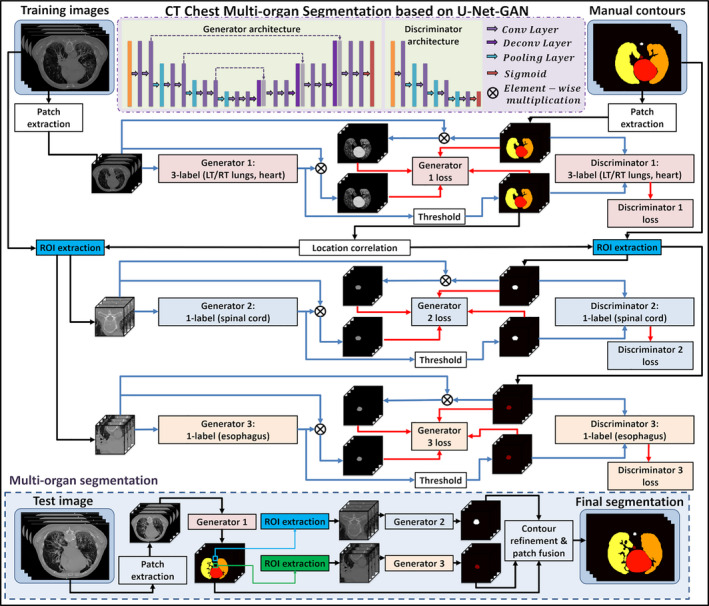
Schematic flowchart of the proposed algorithm for thoracic computed tomography (CT) multiorgan segmentation. The upper part (white) shows the training stage of the proposed method, which consists of three generative adversarial networks (GANs). The lower part (light blue) shows the segmentation stage. In segmenting stage, CT patches are fed into the three well‐trained models to get organ‐at‐risk segmentations. [Color figure can be viewed at wileyonlinelibrary.com]

In the segmentation stage, patches consisting of four continuous slices were first extracted from new CT images and fed into the first segmentation model to obtain the heart, left lung and right lung contours. Then, the ROIs of esophagus and spinal cord were cropped based on the lung contours generated by the first model. 3D ROI patches were fed into the well‐trained second and third segmentation models to get the end‐to‐end esophagus and spinal cord contour segmentation, respectively. Finally, all the segmentations had their respective locations determined based on the spatial information of the original CT patches. The OAR contours are reconstructed with patch fusion and refined by contour refinement, such as filling holes, eroding, and dilating operations.

2.A. Data

The 35 sets of thoracic CT images used in this study are obtained from 2017 AAPM Thoracic Auto‐segmentation Challenges.^{35, 36, 37} Each scan contains the entire thoracic region, and manual contours are delineated according to RTOG1106 guidelines. The detailed descriptions of the datasets can be found in references.^{35, 36}

2.B. Generative adversarial network

Due to the contrast limitation of CT images, manual contouring, especially contouring around organ boundaries, is prone to interobserver variability. Since manual contours serve as the targets of the segmentation network, the contouring variability results in instability of end‐to‐end network models, such as U‐Net. GAN models take an end‐to‐end network as a generator and introduce extra judgment with a discriminator to help the generator find the optimal solutions. As illustrated in Fig. 2, GAN‐based segmentation model consists of a generator network and a discriminator network. The two networks were optimized one after the other in a zero‐sum game framework. The generator's training objective is to increase the judgment error of the discriminative network (i.e., “fool” the discriminator by producing novel segmented contours that are indistinguishable from manual contours). The discriminator's training objective is to decrease the judgment error of the discriminator network and enhance the ability of differentiating the real from the fake. Back‐propagation is applied in both networks so that the generator produces more realistic segmentation, while the discriminator becomes more skilled at flagging segmented contours against manual contours. Therefore, we applied this well‐known network, GAN, in our algorithm.

Figure 2.

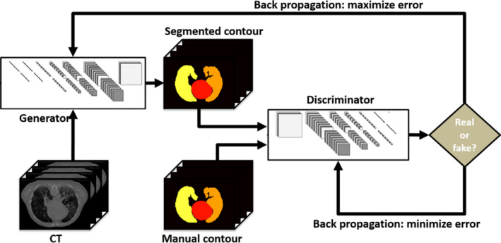
An example illustrating the process of generative adversarial network. [Color figure can be viewed at wileyonlinelibrary.com]

The details of the proposed GAN model are illustrated as follows. The CT patches were fed into the generator network, U‐Net,²⁹ to get the end‐to‐end segmented contours. As shown in generator architecture part of Fig. 1, the generator network consists of a compression path (left side), decompression path (right side), and a bridge path (middle side) connecting these two paths. The compression path is composed of two convolutional layers followed by a pooling layer to reduce the resolution. In each convolution layer, feature representations can be extracted via 3D convolutions followed by the parametric rectified linear unit (PReLU). The decompression path is constructed by two convolutional layers followed by a deconvolutional layer to enhance the resolution. The decompression path has a similar structure to the compression path, except that the compression path has no strided convolution. The decompression path uses a bridge path to concatenate features from equal‐sized compression and decompression paths. U‐Net with such concatenation, that is, a dense block network, encourages each path to obtain both high‐frequency information (such as textural information) and low‐frequency information (such as structural information) to represent the image patch. In order to output equal‐sized segmented contour probability maps, deconvolutions with 2 × 2 × 2 stride size are used. At the end of the generator, probability maps of contours are generated with soft‐max operators. A threshold was used to binarize the probability maps to binary masks of contours, called as generated contours. Then, as shown in discriminator architecture part, the discriminator was used to judge the authenticity of generated contours against the reference manual contours. The discriminator is a typical classification‐based FCN, which consists of several convolution layers, each of which was followed by a pooling layer. The discriminator outputs a 1 × 1 × 1 variable with 1 denoting real and 0 denoting fake.

The generator loss was computed as the sum of mean squared error (MSE) of the “residual” images, and the binary cross entropy loss of contour images. The “residual” images are calculated as the element‐wise multiplication of the original CT patches with the probability maps of generated contours, and the reference “residual” images are calculated as the multiplication of CT patches and segmentation masks generated by manual contouring. The binary cross entropy is used as the discriminator loss. An Adam optimizer for gradient descent was applied to minimize these two losses. The generator and discriminator are implemented with the TensorFlow python toolbox. Batch sizes are set to 40 for the 2.5D network and 20 for the 3D networks. The training for the three GANs ran for 180 epochs, which took 2 h for the first network and 3.5 h for the second and third networks on a Titan XP 12 GB GPU. The network training normally converges after 100 epochs, and we added more epochs for robustness.

2.C. Residual loss for generator optimization

During training, traditional generators use similarity or dissimilarity loss functions, for example, binary cross entropy or Dice loss to compute the generator loss. However, since the region sizes between different labels are usually different, putting them together in one loss will be unfair. Therefore, we propose to use residual loss to cope with this unfairness. The “residual” images are generated by computing the element‐wise multiplication of probability maps of generated contours and original CT patches. The MSE of the “residual” images is combined with binary cross entropy loss of contour images to compute the generator loss.

2.D. Evaluation

We implemented the proposed method on 35 sets of thoracic CT images with leave‐one‐out cross validation. In other words, we had 34 sets of images for training and validation and the remaining set for testing. The proposed network was run 35 times and generated 35 sets of test results. The performance of the proposed method was quantified with six metrics: dice similarity coefficient (DSC), sensitivity, specificity, 95% Hausdorff distance (HD95), mean surface distance (MSD), and residual mean square deviation (RMSD). DSC calculates the overlapping of ground truth contours and the contours generated with proposed method,

$$DSC=\frac{2\times |X\cap Y|}{|X|+|Y|}$$ (1)

where X and Y are the ground truth contours and the contours obtained with proposed method, respectively. Sensitivity and specificity quantify the overlapping ratio inside and outside the ground truth volume,

$$Sensitivity=\frac{|X\cap Y|}{|X|}$$ (2)

$$Specificity=\frac{|\overline{X}\cap \overline{Y}|}{|\overline{X}|}$$ (3)

where $\overline{X}$ and $\overline{Y}$ are the volumes outside the ground truth contours and autosegmented contours, respectively. Mean surface distance (MSD) calculates the average of two directed mean surface distances,

$$MSD=\frac{{\overrightarrow{d}}_{H,avg}(X,Y)+{\overrightarrow{d}}_{H,avg}(Y,X)}{2}$$ (4)

where directed mean surface distance is ${\overrightarrow{d}}_{H,avg}(X,Y)=\frac{1}{|X|}{\sum }_{x\in |X|}{min}_{y\in |Y|}d(x,y)$, calculating the average distance of a point in X to its nearest neighbor in Y. Directed 95% Hausdorff distance measures the 95th percentile distance of all distances between points in X and the nearest point in Y, ${\overrightarrow{d}}_{H,avg}(X,Y)=K_{95}\left(mi{n}_{y\in |Y|}d(x,y)\right)$. HD95 is calculated as the mean of two directed 95% Hausdorff distances,

$$HD95=\frac{{\overrightarrow{d}}_{H,95}(X,Y)+{\overrightarrow{d}}_{H,95}(Y,X)}{2}$$ (5)

Residual mean square deviation calculates the residual mean square distance between segmented contour and manual contour. RMSD is calculated as

$$\begin{array}{cc}& \mathit{RMSD}\hfill \\ & =\sqrt{\frac{1}{|X|}{\sum }_{x\in |X|}\underset{y\in |Y|}{min}d{(x,y)}^2+\frac{1}{|Y|}{\sum }_{y\in |Y|}\underset{x\in |x|}{min}d{(y,x)}^2}\hfill \end{array}$$ (6)

To evaluate the dosimetric impact of the proposed autosegmentation method, we made 20 lung SBRT plans with ground truth contours and planning target volume (PTV) which are defined on abnormal spots in lungs on each CT image dataset. We then calculated the dose‐volume histogram (DVH) differences between ground truth contours and autosegmented contours. Compared to conventional fractionated radiotherapy, SBRT usually demonstrates sharper dose drop‐off, thus demanding higher delineation accuracy. Therefore, the evaluation plans are made according to SBRT guidance. All 20 plans are prescribed to 10 Gy per fraction for five fractions and normalized as 100% prescription dose to 95% of PTV volume. We calculated Dmean, D95, D50, D5, Dmin, and Dmax differences between ground truth contours and autosegmented contours to access the clinical feasibility of the proposed method. For total lungs, we also calculated more clinically relevant dose metrics, D1000 cc, and D1500 cc.

3. Results

Figures 3 and 4 show the 2D and 3D segmentation results on one patient using the proposed U‐Net‐GAN method. The proposed method segments bilateral lungs, heart, and spinal cord, and successfully delineates the esophagus. The OARs obtained with our method show great resemblance to the ground truth contours.

Figure 3.

(a) Three transverse computed tomography slices on one patient and the corresponding organ‐at‐risk contours obtained from (b) manual contouring (ground truth) and (c) the proposed method. [Color figure can be viewed at wileyonlinelibrary.com]

Figure 4.

3D visualization the organ‐at‐risk contours on the same patient in Fig. 3 obtained with (a) manual contouring and (b) the proposed method. [Color figure can be viewed at wileyonlinelibrary.com]

The quantitative evaluation results are summarized in Fig. 5 and Table 1. Figure 5 shows six evaluation metrics — DSC, sensitivity, specificity, HD95, MSD, and RMSD — calculated on all 35 patients, and their mean and standard deviation are listed in Table 1. As illustrated in Fig. 5 and Table 1, the proposed method achieves superior segmentation accuracy on the left lung, right lung and spinal cord, with respective mean DSC of 0.97, 0.97, and 0.90, mean HD95 of 2.07, 2.50, and 1.19 mm, and all average MSD less than 1 mm. Heart segmentation is not as straightforward as lung and spinal cord segmentation due to the reduced image contrast. The quantitative evaluations demonstrate close matching of the proposed method and the ground truth on heart delineation. The mean DSC is 0.87, mean HD95 is 4.58 mm, and mean MSD is 1.49 mm. Esophagus is of the lowest contrast among the five OARs on CT images, thus the most difficult one to delineate. The proposed method obtains 0.75 ± 0.08 DSC, 4.52 ± 3.81 mm HD95, and 1.05 ± 0.66 mm MSD on esophagus segmentation. Sensitivity evaluates the true OAR volume overlapped by the volume obtained from the proposed method, and specificity quantifies the overlapped portion outside the true volume. The proposed method achieves average segmentation sensitivity of 0.74–0.97, with the highest on bilateral lungs, and the lowest on esophagus. Specificity of all five OARs is close to unity. The mean RMSD ranges from 0.8 to 3.1 mm on the five OARs.

Figure 5.

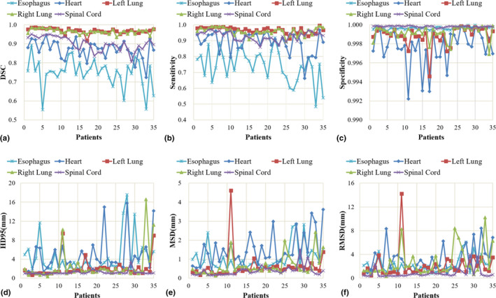
The six evaluation metrics, (a) dice similarity coefficient, (b) Sensitivity, (c) Specificity, (d) 95% Hausdorff distance, (e) mean surface distance, and (f) residual mean square deviation of the five organs‐at‐risk calculated on 35 patients. [Color figure can be viewed at wileyonlinelibrary.com]

Table 1.

Mean and standard deviation of DSC, sensitivity, specificity, HD95, MSD, and RMSD. The minimum and maximum values are listed in parentheses

	Esophagus	Heart	Left lung	Right lung	Spinal cord
DSC	0.75 ± 0.08	0.87 ± 0.05	0.97 ± 0.01	0.97 ± 0.01	0.90 ± 0.04
	(0.55, 0.89)	(0.72, 0.95)	(0.92, 0.99)	(0.93, 0.99)	(0.81, 0.95)
Sensitivity	0.74 ± 0.10	0.89 ± 0.07	0.97 ± 0.02	0.96 ± 0.02	0.93 ± 0.03
	(0.48, 0.92)	(0.66, 0.97)	(0.91, 0.998)	(0.90, 0.99)	(0.86, 0.97)
Specificity	0.9997 ± 0.0001	0.9977 ± 0.0020	0.9989 ± 0.0010	0.9992 ± 0.0007	0.9998 ± 0.00001
	(0.9993, 0.9997)	(0.9922. 0.9999)	(0.9946, 0.9999)	(0.9969, 0.9999)	(0.9996, 0.99995)
HD95 (mm)	4.52 ± 3.81	4.58 ± 3.67	2.07 ± 1.93	2.50 ± 3.34	1.19 ± 0.46
	(1.58, 17.56)	(1.33, 15.77)	(0.67, 9.43)	(0.33, 16.58)	(0.67, 3.50)
MSD (mm)	1.05 ± 0.66	1.49 ± 0.85	0.61 ± 0.73	0.65 ± 0.53	0.38 ± 0.27
	(0.46, 2.83)	(0.40, 3.62)	(0.16, 4.62)	(0.13, 2.43)	(0.15, 1.51)
RMSD (mm)	2.24 ± 1.36	3.14 ± 2.19	2.12 ± 2.32	2.66 ± 2.46	0.82 ± 0.85
	(0.82, 6.03)	(0.82, 8.39)	(0.46, 14.24)	(0.35, 10.24)	(0.33, 3.95)

DSC: dice similarity coefficient; HD95: 95% Hausdorff distance; MSD: mean surface distance; RMSD: residual mean square deviation.

Figure 6 shows linear regression analysis between ground truth and the proposed methods of the five OAR volumes. The linear correlation, R ², is larger than 0.84, and all P < 0.001, which indicates strong statistical correlations between the ground truth volumes and those obtained with the proposed method.

Figure 6.

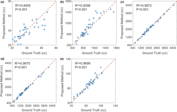
Linear regression analysis of (a) esophagus, (b) heart, (c) left lung, (d) right lung, and (e) spinal cord volumes obtained with manual contouring (ground truth) and proposed method. Blue circles indicate individual patient measurement, and the dashed red line is the line of identity. [Color figure can be viewed at wileyonlinelibrary.com]

We also evaluate the dosimetric impact of the contours obtained with the proposed automatic segmentation method. As shown in Fig. 7, the DVH of the all five OARs of an exemplary patient obtained from manual contouring and the proposed method match well. We calculated Dmean, D95, D50, D5, Dmin, and Dmax differences on all five OARs obtained from manual contouring and the proposed method for all 20 plans. The mean, standard deviation, and corresponding P‐value of dose differences calculated on ground truth OAR doses and autosegmented OAR doses are summarized in Table 2. Twenty‐six of all 32 dosimetric metrics show P > 0.05, indicating no statistically significant dose differences between ground truth OAR and autosegmented OAR. The mean differences of Dmean, D95, D50, D5, and Dmin of all five OARs are all less than 0.7 Gy. The mean Dmax differences range from −0.06 to 1.5 Gy. The average dose differences on D1000 cc and D1500 cc of total lung are less than 0.02 Gy, with both P > 0.05.

Figure 7.

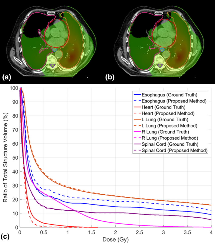
Dose distribution on one patient with (a) ground truth contours and (b) autosegmented contours, and (c) the corresponding dose‐volume histograms. Window width for (a) and (b): 0.1–1 Gy. [Color figure can be viewed at wileyonlinelibrary.com]

Table 2.

The mean and standard deviation (SD) of dose differences and P‐value calculated with ground truth organs‐at‐risk (OARs) dose and autosegmented OARs dose on 20 stereotactic body radiation therapy plans

	Dmin	D95	D50	D5	Dmean	Dmax
Esophagus
Mean (Gy)	0.010	0.012	0.048	0.213	0.145	1.003
SD (Gy)	0.016	0.017	0.068	0.626	0.240	2.740
P‐value	0.012	0.007	0.005	0.146	0.014	0.118
Heart
Mean (Gy)	−0.001	−0.002	0.002	0.280	0.056	0.247
SD (Gy)	0.006	0.010	0.028	1.092	0.173	2.926
P‐value	0.528	0.385	0.815	0.266	0.162	0.710
Left lung
Mean (Gy)	0.003	0.005	0.014	0.063	0.025	0.147
SD (Gy)	0.012	0.009	0.054	0.222	0.059	0.871
P‐value	0.254	0.035	0.257	0.219	0.073	0.461
Right lung
Mean (Gy)	−0.002	0.004	0.027	0.668	0.155	1.527
SD (Gy)	0.023	0.001	0.118	1.698	0.341	2.924
P‐value	0.695	0.088	0.319	0.095	0.057	0.031
Spinal cord
Mean (Gy)	0	0.001	0.002	0.028	‐0.001	‐0.055
SD (Gy)	0	0.002	0.015	0.144	0.065	0.203
P‐value	N/A	0.330	0.659	0.394	0.973	0.241
	D1000 cc	D1500 cc
Total lung
Mean (Gy)	0.017	0.005
SD (Gy)	0.043	0.025
P‐value	0.095	0.427

4. Discussion

Target and OAR delineation is the prerequisite for treatment planning, especially for highly conformal radiotherapy, since those treatment plans are optimized and evaluated based on the dose constraints on targets and OARs. Delineation accuracy directly impacts the quality of treatment plans. Manual contouring suffers from the notorious inter‐ and intraobserver variability, and contouring quality highly depends on the expertise and experience of clinicians. The proposed automatic segmentation method provides accurate and consistent organ delineations that are independent of observers. While manual contouring usually takes from about half an hour to several hours depending on anatomical sites, the well‐trained automatic segmentation method can finish multiple OAR contouring in several seconds. This greatly shortens the preparation process for treatment planning, and the saved time can be used to either obtain a better treatment plan or accelerate the treatment of fast‐growing tumors. Automatic segmentation also shows the potential to facilitate online adaptive radiotherapy (ART). Online ART adapts the daily changes with patients on table. The entire process, from daily imaging to organ contouring, replanning, and planning QA, needs to conclude in 10–20 min, therefore, it is desirable to minimize the processing time for each step. The proposed method was performed on an NVIDIA TITAN XP GPU with 12 GB of memory and segments all five organs within 6 s. With the help of more powerful GPUs, the segmentation time could be further reduced.

The U‐Net‐GAN improves upon the U‐Net approach by introducing a discriminator. To offer a concrete display of improvement, we conducted a leave‐one‐out experiment to compare the results generated by U‐Net with and without the adversarial network, shown in Table 3. All parameters of U‐Net were set based on the parameters that offered the best performance. As shown in the table, with the help of the adversarial network, majorities of the evaluation metrics are improved (DSC, Specificity and Sensitivity increased; HD95, MSD, and RMSD decreased).

Table 3.

The segmentation comparison between U‐Net and U‐Net–generative adversarial network (U‐Net‐GAN), the proposed method, with the mean and standard deviation of dice similarity coefficient (DSC), sensitivity, specificity, 95% Hausdorff distance (HD95), mean surface distance (MSD), and residual mean square deviation (RMSD) listed

	Esophagus	Heart	Left lung	Right lung	Spinal cord
DSC
U‐Net	0.71 ± 0.08	0.85 ± 0.05	0.97 ± 0.01	0.96 ± 0.01	0.83 ± 0.05
U‐Net‐GAN	0.75 ± 0.08	0.87 ± 0.05	0.97 ± 0.01	0.97 ± 0.01	0.90 ± 0.04
Sensitivity
U‐Net	0.71 ± 0.09	0.94 ± 0.05	0.97 ± 0.02	0.96 ± 0.02	0.97 ± 0.01
U‐Net‐GAN	0.73 ± 0.10	0.89 ± 0.07	0.97 ± 0.02	0.96 ± 0.02	0.93 ± 0.03
Specificity
U‐Net	0.9996 ± 0.0002	0.9958 ± 0.0029	0.9989 ± 0.0010	0.9992 ± 0.0007	0.9995 ± 0.0001
U‐Net‐GAN	0.9997 ± 0.0001	0.9977 ± 0.0020	0.9989 ± 0.0010	0.9992 ± 0.0007	0.9998 ± 0.00001
HD95 (mm)
U‐Net	4.91 ± 4.13	6.45 ± 4.03	2.07 ± 1.92	2.50 ± 3.33	1.98 ± 1.52
U‐Net‐GAN	4.52 ± 3.81	4.58 ± 3.67	2.07 ± 1.93	2.50 ± 3.34	1.19 ± 0.46
MSD (mm)
U‐Net	1.09 ± 0.67	1.91 ± 0.95	0.61 ± 0.73	0.65 ± 0.53	0.54 ± 0.29
U‐Net‐GAN	1.05 ± 0.66	1.49 ± 0.85	0.61 ± 0.73	0.65 ± 0.53	0.38 ± 0.27
RMSD (mm)
U‐Net	2.37 ± 1.40	3.68 ± 2.24	2.12 ± 2.32	2.66 ± 2.45	1.08 ± 1.32
U‐Net‐GAN	2.24 ± 1.36	3.14 ± 2.19	2.12 ± 2.32	2.66 ± 2.46	0.82 ± 0.85

The datasets used in this work are obtained from 2017 AAPM Thoracic Auto‐segmentation Challenges. Reference ³⁵ shows the segmentation results from seven institutes. Five of seven institutes developed deep learning‐based methods, and the other two (institute #4 and #6) used multiatlas‐based methods. We compared the segmentation results using our proposed method with results from the seven groups and listed the comparison results in Table 4. Our method generates similar DSC on bilateral lungs, heart, and spinal cord, but outperforms all seven methods on esophagus segmentation. MSD and HD95 obtained with proposed method are superior to all seven methods on all five OARs.

Table 4.

The segmentation comparison of the proposed method with the seven methods participated in 2017 AAPM thoracic autosegmentation challenges

	Method	Esophagus	Heart	Left Lung	Right lung	Spinal cord
DSC	1	0.72 ± 0.10	0.93 ± 0.02	0.97 ± 0.02	0.97 ± 0.02	0.88 ± 0.037
	2	0.64 ± 0.20	0.92 ± 0.02	0.98 ± 0.01	0.97 ± 0.02	0.89 ± 0.042
	3	0.71 ± 0.12	0.91 ± 0.02	0.98 ± 0.02	0.97 ± 0.02	0.87 ± 0.110
	4	0.64 ± 0.11	0.90 ± 0.03	0.97 ± 0.01	0.97 ± 0.02	0.88 ± 0.045
	5	0.61 ± 0.11	0.92 ± 0.02	0.96 ± 0.03	0.95 ± 0.05	0.85 ± 0.035
	6	0.58 ± 0.11	0.90 ± 0.02	0.96 ± 0.01	0.96 ± 0.02	0.87 ± 0.022
	7	0.55 ± 0.20	0.85 ± 0.04	0.95 ± 0.03	0.96 ± 0.02	0.83 ± 0.080
	Proposed	0.75 ± 0.08	0.87 ± 0.05	0.97 ± 0.01	0.97 ± 0.01	0.90 ± 0.04
MSD (mm)	1	2.23 ± 2.82	2.05 ± 0.62	0.74 ± 0.31	1.08 ± 0.54	0.73 ± 0.21
	2	6.30 ± 9.08	2.42 ± 0.82	0.61 ± 0.26	0.93 ± 0.53	0.69 ± 0.25
	3	2.08 ± 1.94	2.98 ± 0.93	0.62 ± 0.35	0.91 ± 0.52	0.76 ± 0.60
	4	2.03 ± 1.94	3.00 ± 0.96	0.79 ± 0.27	1.06 ± 0.63	0.71 ± 0.25
	5	2.48 ± 1.15	2.61 ± 0.69	2.90 ± 6.94	2.70 ± 4.84	1.03 ± 0.84
	6	2.63 ± 1.03	3.15 ± 0.85	1.16 ± 0.43	1.39 ± 0.61	0.78 ± 0.14
	7	13.10 ± 10.39	4.55 ± 1.59	1.22 ± 0.61	1.13 ± 0.49	2.10 ± 2.49
	Proposed	1.05 ± 0.66	1.49 ± 0.85	0.61 ± 0.73	0.65 ± 0.53	0.38 ± 0.27
HD95 (mm)	1	7.3 ± 10.31	5.8 ± 1.98	2.9 ± 1.32	4.7 ± 2.50	2.0 ± 0.37
	2	19.7 ± 25.90	7.1 ± 3.73	2.2 ± 10.79	3.6 ± 2.30	1.9 ± 0.49
	3	7.8 ± 8.17	9.0 ± 4.29	2.3 ± 1.30	3.7 ± 2.08	2.0 ± 1.15
	4	6.8 ± 3.93	9.9 ± 4.16	3.0 ± 1.08	4.6 ± 3.45	2.0 ± 0.62
	5	8.0 ± 3.80	8.8 ± 5.31	7.8 ± 19.13	14.5 ± 34.4	2.3 ± 0.50
	6	8.6 ± 3.82	9.2 ± 3.10	4.5 ± 1.62	5.6 ± 3.16	2.1 ± 0.35
	7	37.0 ± 26.88	13.8 ± 5.49	4.4 ± 3.41	4.1 ± 2.11	8.1 ± 10.72
	Proposed	4.52 ± 3.81	4.58 ± 3.67	2.07 ± 1.93	2.50 ± 3.34	1.19 ± 0.46

Bold indicates is best values.

To evaluate the dosimetric impact of the autosegmented contours, we made 20 Lung SBRT plans with ground truth contours and compared the dose of OARs from manual contouring and autocontouring. Among the 32 evaluation dose metrics, 29 metrics calculate the average dose difference to be less than 0.5 Gy, and 24 calculate the difference to be less than 0.1 Gy. Twenty‐six of 32 metrics have P‐value larger than 0.05, indicating no statistically significant differences. For the six dose metrics with P‐value smaller than 0.05, Table 5 lists their mean dose values on both ground truth contours and autosegmented contours. The esophagus Dmin, D95, D50, Dmean, and left lung D95 on both ground truth contours and autosegmented contours are all less 1.4 Gy, and the dose differences are less than 0.2 Gy. Although the P‐values are less than 0.05, the dose differences of 0.03–0.2 Gy are minimal. The average Dmax difference for right lung is 1.527 Gy with P‐value of 0.03. Dmax is sensitive to contour edges, especially when OAR lies in the region of sharp dose drop‐off. Sixteen out of the 20 plans have PTV lying in the right lung, therefore, it is within expectation that the Dmax as well as Dmax differences in right lung are larger than those of other OARs. As shown in Table 5, the average Dmax of right lung is 44.4, and 1.5 Gy counts only for 3.4% relative difference. Moreover, clinicians place more emphasis on D1000 cc and D1500 cc of total lung when evaluating SBRT plans, and these two metrics show very minimal difference (<0.02 Gy, P > 0.05).

Table 5.

The average dose on ground truth contours and autosegmented contours, and corresponding differences for the six dose‐volume histogram (DVH) metrics with P < 0.05 listed in Table II

	Esophagus	Esophagus	Esophagus	Esophagus	Left lung	Right lung
	Dmin	D95	D50	Dmean	D95	Dmax
Ground truth (Gy)	0.030	0.053	0.278	1.222	0.080	43.447
The proposed (Gy)	0.040	0.064	0.326	1.367	0.084	44.964
Difference (Gy)	0.010	0.012	0.048	0.145	0.005	1.527

Compared to atlas‐based and model‐based methods, deep learning‐based methods are developed on large amounts of data with a substantial number of features, and therefore, have the potential to provide a better solution for problems with large variations. In applying the established image segmentation methods in computer vision to medical imaging, the first challenge is the lack of training data. Those established methods are built on anywhere from several thousand up to several million training samples, which is impractical for medical imaging. In this work, with leave‐one‐out cross validation, only 34 sets of thoracic CT are available for training. To supplement training data, we applied data augmentation techniques, such as shifting, mirroring, flipping, scaling, and rotation on the available CT images.²⁹ With intensive augmentation, the performance of the proposed method tends to stabilize when more than 20 sets of CT data are used for training. This approach also has realistic indications. Patient movement, such as translation and rotation, does not change the relative position between organs. Including the transformed data could help avoid overfitting and help the segmentation algorithm learn this invariant property.

It is worth noting that the performance of the proposed method is not uniform across all 35 patients. The segmentation accuracy for some patients, such as patient #11, #17, and #33, is inferior to others. Patient #11 suffered left lung collapse, and right lung extended across the midline. The proposed method mislabeled part of the right lung as left lung. Patient #17 and #33 had large lung lesions, and the proposed method labeled the lesions differently from manual contouring. As noted, the proposed network tends to mislabel organs when unusual structures exist. This issue can be alleviated by including more diverse and variable data for training.

Due to the dimension differences and variation between patients, it is difficult to balance the loss function between the four organs. Integrating all the segmentations into one network complicates the training process and reduces segmentation accuracy. To simplify the method, we group OARs of similar dimensions, and utilize three subnetworks for segmentation, one for lungs and heart, and the other two for esophagus and spinal cord, respectively. This approach improves segmentation accuracy at the cost of computation efficiency. It could be an issue if we want to apply the proposed method to segment more OARs. In the future, we will explore the possibility of multiple organ segmentation in a single network.

Manual contouring uncertainty causes errors in plan optimization and results in nonoptimal or unacceptable plans. Fiorino et al. performed a study on the intra‐ and interobserver variation in prostate and seminal vesicles delineation, and found that 2–3 mm contouring variation resulted in 4% and 12% variation in mean dose on bladder and rectum, and 10% uncertainty on volume received 95% prescription doses.³⁸ Nelms et al. also observed substantial dosimetric impacts due to OAR contouring variation on a head and neck patient, where the mean dose ranged from −289% to 56%, and maximum dose from −22% to 35%.¹⁰ Similar uncertainty was observed for brachytherapy, where OAR contouring variation resulted in 10% uncertainty in D2 cc.³⁹ In this work, we assessed the feasibility of using autosegmented contours to evaluate treatment plans. To further validate the daily clinical implementation of the proposed method, we will evaluate the reliability of treatment planning using autosegmented contours.

5. Conclusion

We have investigated a novel deep learning‐based approach with a GAN strategy to segment multiple OARs in the thorax using chest CT images. Experimental validation has been performed to demonstrate its clinical feasibility and reliability. This multiple OAR segmentation could be a useful tool for improving the efficiency of the lung radiotherapy treatment planning.

Conflict of interest

No potential conflict of interest relevant to this article exists.

References

- 1. Miller KD, Siegel RL, Lin CC, et al. Cancer treatment and survivorship statistics, 2016. CA Cancer J Clin. 2016;66:271–289. [DOI] [PubMed] [Google Scholar]
- 2. Cronin KA, Lake AJ, Scott S, et al. Annual report to the nation on the status of cancer, part I: national cancer statistics. Cancer. 2018;124:2785–2800. [DOI] [PMC free article] [PubMed] [Google Scholar]
- 3. Siegel RL, Miller KD, Jemal A. Cancer statistics, 2018. CA Cancer J Clin. 2018;68:7–30. [DOI] [PubMed] [Google Scholar]
- 4. Liao Z, Lee JJ, Komaki R, et al. Bayesian adaptive randomization trial of passive scattering proton therapy and intensity‐modulated photon radiotherapy for locally advanced non‐small‐cell lung cancer. J Clin Oncol. 2018;36:1813–1822. [DOI] [PMC free article] [PubMed] [Google Scholar]
- 5. Hurkmans CW, Borger JH, Pieters BR, Russell NS, Jansen EP, Mijnheer BJ. Variability in target volume delineation on CT scans of the breast. Int J Radiat Oncol Biol Phys. 2001;50:1366–1372. [DOI] [PubMed] [Google Scholar]
- 6. Rasch C, Steenbakkers R, van Herk M. Target definition in prostate, head, and neck. Semin Radiat Oncol. 2005;15:136–145. [DOI] [PubMed] [Google Scholar]
- 7. Van de Steene J, Linthout N, de Mey J, et al. Definition of gross tumor volume in lung cancer: inter‐observer variability. Radiother Oncol. 2002;62:37–49. [DOI] [PubMed] [Google Scholar]
- 8. Vinod SK, Jameson MG, Min M, Holloway LC. Uncertainties in volume delineation in radiation oncology: a systematic review and recommendations for future studies. Radiother Oncol. 2016;121:169–179. [DOI] [PubMed] [Google Scholar]
- 9. Breunig J, Hernandez S, Lin J, et al. A system for continual quality improvement of normal tissue delineation for radiation therapy treatment planning. Int J Radiat Oncol Biol Phys. 2012;83:e703–e708. [DOI] [PubMed] [Google Scholar]
- 10. Nelms BE, Tome WA, Robinson G, Wheeler J. Variations in the contouring of organs at risk: test case from a patient with oropharyngeal cancer. Int J Radiat Oncol Biol Phys. 2012;82:368–378. [DOI] [PubMed] [Google Scholar]
- 11. Isgum I, Staring M, Rutten A, Prokop M, Viergever MA, van Ginneken B. Multi‐atlas‐based segmentation with local decision fusion–application to cardiac and aortic segmentation in CT scans. IEEE Trans Med Imaging. 2009;28:1000–1010. [DOI] [PubMed] [Google Scholar]
- 12. Aljabar P, Heckemann RA, Hammers A, Hajnal JV, Rueckert D. Multi‐atlas based segmentation of brain images: atlas selection and its effect on accuracy. NeuroImage. 2009;46:726–738. [DOI] [PubMed] [Google Scholar]
- 13. Iglesias JE, Sabuncu MR. Multi‐atlas segmentation of biomedical images: a survey. Med Image Anal. 2015;24:205–219. [DOI] [PMC free article] [PubMed] [Google Scholar]
- 14. Ecabert O, Peters J, Schramm H, et al. Automatic model‐based segmentation of the heart in CT images. IEEE Trans Med Imaging. 2008;27:1189–1201. [DOI] [PubMed] [Google Scholar]
- 15. Qazi AA, Pekar V, Kim J, Xie J, Breen SL, Jaffray DA. Auto‐segmentation of normal and target structures in head and neck CT images: a feature‐driven model‐based approach. Med Phys. 2011;38:6160–6170. [DOI] [PubMed] [Google Scholar]
- 16. Sun S, Bauer C, Beichel R. Automated 3‐D segmentation of lungs with lung cancer in CT data using a novel robust active shape model approach. IEEE Trans Med Imaging. 2012;31:449–460. [DOI] [PMC free article] [PubMed] [Google Scholar]
- 17. LeCun Y, Bengio Y, Hinton G. Deep learning. Nature. 2015;521:436–444. [DOI] [PubMed] [Google Scholar]
- 18. Krizhevsky A, Sutskever I, Hinton GE. ImageNet classification with deep convolutional neural networks. In: NIPS; 2012.
- 19. Girshick R, Donahue J, Darrell T, Malik J. Rich feature hierarchies for accurate object detection and semantic segmentation. arXiv:1311.2524; 2013.
- 20. Sermanet P, Eigen D, Zhang X, Mathieu M, Fergus R, LeCun T. OverFeat: integrated recognition, localization and detection using convolutional networks. arXiv:1312.6229; 2014.
- 21. Shelhamer E, Long J, Darrell T. Fully convolutional networks for semantic segmentation. IEEE Trans Pattern Anal Mach Intell. 2017;39:640–651. [DOI] [PubMed] [Google Scholar]
- 22. He K, Gkioxari G, Dollár P, Girshick R. Mask R‐CNN. arXiv:1703.06870; 2017. [DOI] [PubMed]
- 23. Wang T, Lei Y, Tang H, et al. A learning‐based automatic segmentation and quantification method on left ventricle in gated myocardial perfusion SPECT imaging: a feasibility study. J Nucl Cardiol. 2019;1–12. [Epub ahead of print] 10.1007/s12350-019-01594-2. [DOI] [PMC free article] [PubMed] [Google Scholar]
- 24. Yang X., Huang J., Lei Y., et al. Med‐A‐Nets: Segmentation of Multiple Organs in Chest CT Image with Deep Adversarial Networks. Med Phys. 2018;45:E154‐E154. [Google Scholar]
- 25. Yang X., Lei Y., Wang T., et al. 3D Prostate Segmentation in MR Image Using 3D Deeply Supervised Convolutional Neural Networks. Med Phys. 2018;45:E582‐E583. [Google Scholar]
- 26. Wang B, Lei Y, Tian S, et al. Deeply supervised 3D FCN with group dilated convolution for automatic mri prostate segmentation. Med Phys. 2019; [Epub ahead of print] 10.1002/mp.13416. [DOI] [PMC free article] [PubMed] [Google Scholar]
- 27. Ibragimov B, Xing L. Segmentation of organs‐at‐risks in head and neck CT images using convolutional neural networks. Med Phys. 2017;44:547–557. [DOI] [PMC free article] [PubMed] [Google Scholar]
- 28. Roth HR, Lu L, Farag A, et al. DeepOrgan: Multi‐level deep convolutional networks for automated pancreas segmentation. arXiv:1506.06448; 2015.
- 29. Ronneberger O, Fischer P, Brox T. U‐Net: convolutional networks for biomedical image segmentation. In: Navab N, Hornegger J, Wells W, Frangi A, eds. Medical Image Computing and Computer‐Assisted Intervention – MICCAI 2015. Cham: Springer; 2015:234–241. [Google Scholar]
- 30. Goodfellow IJ, Pouget‐Abadie J, Mirza M, et al. Generative adversarial networks. arXiv:1406.2661; 2014.
- 31. Phillip Isola, Jun‐Yan Zhu, Tinghui Zhou, Alexei A. Efros . Image‐to‐image translation with conditional adversarial networks. arXiv:1611.07004; 2017.
- 32. You C, Li G, Zhang Y, et al. CT super‐resolution GAN constrained by the identical, residual, and cycle learning ensemble (GAN‐CIRCLE). arXiv:1808.04256; 2018. [DOI] [PubMed]
- 33. Wolterink JM, Leiner T, Viergever MA, Isgum I. Generative adversarial networks for noise reduction in low‐dose CT. IEEE Trans Med Imaging. 2017;36:2536–2545. [DOI] [PubMed] [Google Scholar]
- 34. Souly N, Spampinato C, Shah M. Semi Supervised Semantic Segmentation Using Generative Adversarial Network. In: IEEE International Conference on Computer Vision; 2017:5689‐5697.
- 35. Yang J, Veeraraghavan H, Armato SG 3rd, et al. Auto‐segmentation for thoracic radiation treatment planning: a grand challenge at AAPM 2017. Med Phys. 2018;45:4568–4581. [DOI] [PMC free article] [PubMed] [Google Scholar]
- 36. Yang J, Sharp G, Veeraraghavan H, et al. Data from lung CT segmentation challenge. The Cancer Imaging Archive; 2017.
- 37. Clark K, Vendt B, Smith K, et al. The cancer imaging archive (TCIA): maintaining and operating a public information repository. J Digit Imaging. 2013;26:1045–1057. [DOI] [PMC free article] [PubMed] [Google Scholar]
- 38. Fiorino C, Reni M, Bolognesi A, Cattaneo GM, Calandrino R. Intra‐ and inter‐observer variability in contouring prostate and seminal vesicles: implications for conformal treatment planning. Radiother Oncol. 1998;47:285–292. [DOI] [PubMed] [Google Scholar]
- 39. Saarnak AE, Boersma M, van Bunningen BN, Wolterink R, Steggerda MJ. Inter‐observer variation in delineation of bladder and rectum contours for brachytherapy of cervical cancer. Radiother Oncol. 2000;56:37–42. [DOI] [PubMed] [Google Scholar]