Abstract
Purpose
This work aims to develop a new framework of image quality assessment using deep learning‐based model observer (DL‐MO) and to validate it in a low‐contrast lesion detection task that involves CT images with patient anatomical background.
Methods
The DL‐MO was developed using the transfer learning strategy to incorporate a pretrained deep convolutional neural network (CNN), a partial least square regression discriminant analysis (PLS‐DA) model and an internal noise component. The CNN was previously trained to achieve the state‐of‐the‐art classification accuracy over a natural image database. The earlier layers of the CNN were used as a deep feature extractor, with the assumption that similarity exists between the CNN and the human visual system. The PLSR model was used to further engineer the deep feature for the lesion detection task in CT images. The internal noise component was incorporated to model the inefficiency and variability of human observer (HO) performance, and to generate the ultimate DL‐MO test statistics. Seven abdominal CT exams were retrospectively collected from the same type of CT scanners. To compare DL‐MO with HO, 12 experimental conditions with varying lesion size, lesion contrast, radiation dose, and reconstruction types were generated, each condition with 154 trials. CT images of a real liver metastatic lesion were numerically modified to generate lesion models with four lesion sizes (5, 7, 9, and 11 mm) and three contrast levels (15, 20, and 25 HU). The lesions were inserted into patient liver images using a projection‐based method. A validated noise insertion tool was used to synthesize CT exams with 50% and 25% of routine radiation dose level. CT images were reconstructed using the weighted filtered back projection algorithm and an iterative reconstruction algorithm. Four medical physicists performed a two‐alternative forced choice (2AFC) detection task (with multislice scrolling viewing mode) on patient images across the 12 experimental conditions. DL‐MO was operated on the same datasets. Statistical analyses were performed to evaluate the correlation and agreement between DL‐MO and HO.
Results
A statistically significant positive correlation was observed between DL‐MO and HO for the 2AFC low‐contrast detection task that involves patient liver background. The corresponding Pearson product moment correlation coefficient was 0.986 [95% confidence interval (0.950, 0.996)]. Bland–Altman agreement analysis did not indicate statistically significant differences.
Conclusions
The proposed DL‐MO is highly correlated with HO in a low‐contrast detection task that involves realistic patient liver background. This study demonstrated the potential of the proposed DL‐MO to assess image quality directly based on patient images in realistic, clinically relevant CT tasks.
Keywords: computed tomography, CT protocol optimization, deep learning, image quality assessment, model observer
1. Introduction
Quantitative and objective image quality assessment is critical to optimize radiation dose and scanning protocols in clinical CT. Human observer (HO) studies to determine diagnostic performance and clinical image quality are typically limited by cost, efficiency, and intra‐ and interobserver variabilities. Traditional image quality metrics are inappropriate for the newer CT systems when iterative reconstruction (IR) or other nonlinear algorithms are used,1, 2, 3, 4 and thus have limited use in quantifying overall image quality for given diagnostic tasks. The use of mathematical model observers (MOs), as objective and efficient alternatives to HOs,5, 6, 7, 8, 9, 10, 11, 12, 13 have become popular in task‐based CT image quality assessment, due to the limitations of traditional methods and the growing needs for CT protocol optimization. Once MOs are determined to be highly correlated with HOs in clinically relevant tasks, MOs can be used to estimate the HO performance, which is the ultimate measure of diagnostic image quality.
Strong correlation between traditional anthropomorphic MOs and HOs has been demonstrated for low‐contrast object detection, localization, and differentiation tasks in uniform phantom backgrounds with varying experimental conditions.8, 9, 14, 15, 16, 17, 18 Some of these studies performed a simple two‐dimensional (2D) object detection task in 2D static images (i.e., static viewing mode) with real8, 9, 14 or simulated uniform phantom background.17, 18 Other studies15, 16 performed a three‐dimensional object detection task in a uniform phantom background, where readers scrolled through multiple images (i.e., cine viewing mode) to identify lesion‐present cases. Nevertheless, these studies did not include patient anatomical variability and nonuniformity, which may affect HO performance more than stochastic image noise alone.19, 20, 21 Thus, it is not clear if the performance of traditional MOs would be highly correlated with the performance of HOs for realistic tasks in real patient images. This is partially due to the difficulty of obtaining sufficient statistics from the patient images with largely varying anatomical background.
A few recent studies aimed to address the above challenges by developing new MOs based on deep learning techniques that use convolutional neural networks (CNN),22, 23, 24, 25 since CNN is biologically inspired multilayer perceptron that could simulate the human visual cortex. In Alnowami et al.'s work 22 and Massanes et al.'s work,23 CNN‐based MOs achieved object detectability comparable to HOs for detection tasks that involved simulated or clinical mammograms. In Kopp et al.'s study,24 another CNN‐based MO also achieved similar performance to HOs for an object detection task that involved a uniform background in CT phantom images. In Zhou and Anastasio's study,25 a CNN was trained to approximate the ideal observer, using computer‐simulated uniform background with correlated noise. These prior studies constructed MOs as a single CNN model with relatively shallow architecture and these MOs were typically tested using simplistic detection tasks that involved neither complicated anatomical background (e.g., CT chest/liver images) nor the realistic human visual searching process. They did not include calibration steps that are typically used to degrade MO performance to the same level of HO performance. Therefore, the validity of these previous CNN‐based MOs in realistic tasks that involve significant background variability and real visual searching process of radiologists remains unclear.
In this work, we propose to develop a new framework of task‐based image quality assessment using deep learning‐based MO (DL‐MO) that would directly operate on patient CT images. Different from previous CNN‐based MOs, the proposed MO is constructed as an ensemble model via transfer learning strategy. We validate the new DL‐MO in a low‐contrast lesion detection task that involves CT images with patient anatomical background.
2. Materials and methods
2.A. DL‐MO framework
The proposed DL‐MO was constructed as a pipeline of a pretrained CNN, a PLS‐DA model, and an internal noise component (Fig. 1). First, the input images were preprocessed and fed into the pretrained CNN to generate CNN codes (i.e., feature vectors). The preprocessing steps are detailed in Sections 2.B.2 and 2.B.3. Then, CNN codes were further engineered by a PLS‐DA model to generate initial test statistics λ 0. Finally, the internal noise was added to λ 0 to generate the final test statistics λ used for performance analyses. Each component of the proposed DL‐MO is further explained as follows.
Figure 1.
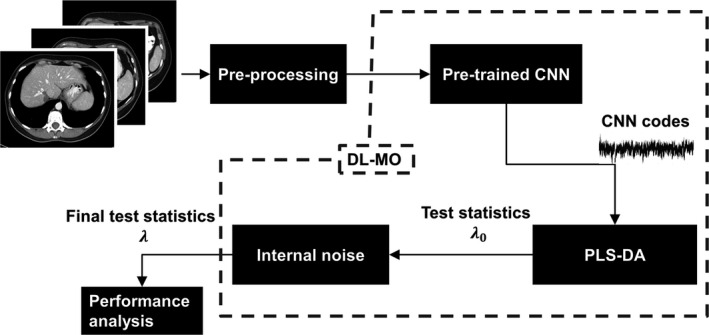
The framework of the proposed deep learning‐based model observer (DL‐MO), including a pretrained deep convolutional neural network (CNN), partial least square regression discriminant analysis (PLS‐DA) model, and internal‐noise component.
2.A.1. Pretrained CNN
In this study, we hypothesized that the state‐of‐the‐art CNN architectures can mimic the feed‐forward information flow and response of human visual system for lesion detection tasks. Given ten thousands of free parameters in these CNNs, direct training of such neural networks from scratch requires a careful preparation of a huge amount of labeled training data to avoid overfitting, which is typically not practical in the field of medical imaging. Thus, we constructed the DL‐MO using the transfer learning strategy, that is, applying the knowledge gained while solving one task to address a different but relevant task.26 Briefly, transfer learning adapts any prior machine learning model (e.g., CNN) pretrained for a pair of source domain D s and source task T s to another pair of target domain D T and target task T T . The prior model defines a functional mapping from D s to T s :
| (1) |
| (2) |
where is the m‐dimensional feature vectors that belong to the source feature space , Pr {X} is the corresponding marginal probability distribution of X, is the n‐dimensional encoded label in the source label space , and Pr {Y|X} is the corresponding conditional probability distribution of Y given X. Then, the prior model is adapted to generate a new mapping from D T to T T :
| (3) |
| (4) |
where , Pr {X ′}, , and are defined similarly as in Eqs. (1) and (2). Of note, represents the intrinsic features that are explored and exploited by the prior model from the input images. Assuming the similarity between D s and D T , the prior model could be used as a fixed feature extractor to generate new features on D T , and a secondary model (e.g., statistical model) can be trained over for T T . The degree of similarity between D s and D T could be evaluated in terms of the image content (e.g., the object types) and the image features that may be relevant to the source/target tasks.
Specifically, when the prior model is a CNN, the feature (also termed as CNN codes) could be directly extracted from any intermediate layer in the network architecture. The selection of CNN layer often follows a generic guideline, that is, the earlier layers are likely to provide domain‐invariant feature, while the later layers tend to generate domain‐specific feature. In this work, we used a 50‐layer Residual net (termed as ResNet‐50)27 as the prior model, which was pretrained over ImageNet 28 (a database of natural images, that is, D s is the natural image domain). As pointed out in Ref. 29, residual net could be interpreted as the encoder part of deep convolutional framelets, and thus, the corresponding CNN codes could be represented in a matrix form:
| (5) |
where H is the Hankel matrix of the input of the layer used for feature extraction, Ψ and denote subsequent local bases (i.e., convolutional filters) in the same residual block (i.e., the fundamental building block in Residual net), ρ(·) is the ReLU (i.e., Rectified linear unit) activation function, and Φ denotes the nonlocal bases (e.g., pooling operator). The Eq. (5) provides the mathematical representation of for the special case that the prior model is Residual net, and thus, the specific form of would vary if a different prior model is used. Furthermore, the local and nonlocal bases are redundant and non‐orthonormal, which results in inner correlation and high dimensionality of . Since inner correlation and high dimensionality could degrade the performance of the secondary model for T T , needs to be further processed by proper feature engineering methods.
2.A.2. PLS‐DA
To construct the secondary model for T T , we selected the PLS‐DA model30, 31 which incorporated the model generation with an embedded feature engineering procedure that addressed the inner correlation and high dimensionality of . Specifically, we used the PLS‐DA that was implemented with the SIMPLS algorithm.32 The basic principle of PLS‐DA is briefly summarized as follows. The input CNN codes were standardized and then represented as a linear form:
| (6) |
where V is the X‐score matrix (i.e., each column is a PLS component), P is the predictor loading matrix, and E is the predictor residual. In this work, T T was considered as a binary classification task, and the ideal model response was also represented as a linear form:
| (7) |
where is the ideal model response for each sample of X’, that is, C is a discrete label vector (C i = 1 for the ith lesion‐present case, and C j = −1 for the jth lesion‐absent case), U is the C‐score matrix (i.e., the linear combination of the responses that has the maximal covariance with the PLS components), Q is the response loading matrix, and F is the response residual. Based on the Eqs. (6) and (7), the loading matrices P and Q are calculated by regressing and C across V and U,32, 33 respectively, that is, and where p j and q j are the jth row of P and Q, respectively, and v j and u j are the jth column of V and U, respectively. In the SIMPLS algorithm, it is assumed that there exists a linear inner relation U = V · D +, where D is a diagonal matrix and is the residual. Furthermore, the SIMPLS algorithm calculates the X‐score matrix V as V = X′ · W, where the weight matrix W is calculated in an iterative process that involves solving the eigenvectors for the successively deflated · C. More details about this process can be found in Ref. 32. Then, a prediction model was created by calculating a regression coefficient vector B that mapped to C as follows:
| (8) |
| (9) |
When the residual terms F, , and are negligible, the model response (also denoted as PLS‐DA model test statistics λ 0), for any new CNN codes from unknown origin can be simply formulated as . Furthermore, is typically a set of continuous values, although the PLS‐DA model was trained with the discrete label vector C. Thus, a decision threshold could be determined to classify the lesion‐present/absent cases.
2.A.3. Internal noise component
The use of internal noise was to model the inefficiency and variability of HO performance in lesion detection task. Specifically, we used the decision variable internal noise as used in the prior works8, 9, 15 that employed the conventional channelized Hotelling observer:
| (10) |
where λ is the final DL‐MO test statistics, α is a constant weighting factor, and denotes a normal random variable with zero expectation and a variance equal to that of PLS‐DA test statistics for lesion‐absent cases (denoted as λ 0,bkg ). The value of α was determined by calibrating DL‐MO performance and HO performance at one preselected experimental condition. After calibration, the same value of α was used in the other conditions.
2.B. Data preparation
Image data were prepared for comparing DL‐MO and HO at different experimental conditions with varying lesion attributes (i.e., size and contrast), radiation dose, and image reconstruction types. The procedure of data preparation is summarized as follows.
2.B.1. CT exam data collection
Routine abdominal CT exams of seven adult patients were selected from our clinical data registry. A staff abdominal radiologist supervised the procedure of case selection. The case selection based on the following inclusion criteria: patients agreed with retrospective usage of their medical records for research purposes; these exams were acquired from the same single‐source 128 slice CT scanner (SOMATOM AS+, Siemens Healthineer, Germany), following a routine abdominal CT protocol used at our institution; these patients were proven to be lesion free via clinical follow‐up. The supervising radiologist excluded the cases that did not meet the inclusion criteria, had fatty liver, and had obese patients. Of note, multiple images of each exam were used to generate the experimental trials for both DL‐MO and HO studies. The major parameters of the scanning and reconstruction protocol are listed in Table 1. A validated noise insertion tool was used to simulate additional CT exams acquired with 50% and 25% of the routine radiation dose.34
Table 1.
Scanning and reconstruction protocol
| Tube voltage | 100–120 kV |
| CTDIvol | 11.6 ± 3.38 mGy |
| Effective mAs | 245.9 ± 40.5 |
| Reconstruction algorithms | WFBP/IR (SAFIRE) |
| Reconstruction kernels | B30/I30‐2 |
| Slice thickness/increment | 3/3 mm |
WFBP: weighted filtered back projection; IR (SAFIRE): iterative reconstruction (sinogram affirmed iterative reconstruction); B30: WFBP reconstruction kernel with medium sharpness; I30‐2: SAFIRE reconstruction kernel with comparable sharpness to B30 and a strength setting of 2.
2.B.2. Data generation for MO and HO studies
The volumetric CT images of a real liver metastatic lesion were numerically modified to create lesion models with four different sizes (5, 7, 9, and 11 mm) and three different contrast levels (15, 20, and 25 HU). These lesion models were inserted into multiple locations in normal patient liver images, using a previously validated projection‐based method.35 The lesion locations were validated by the same supervising radiologist who selected the original cases. The projection data, with inserted noise and lesions, were reconstructed using a weighted filtered back projection algorithm (WFBP)36 and an iterative reconstruction algorithm—sinogram affirmed iterative reconstruction (IR: SAFIRE).37 The major parameters of image reconstruction are also listed in Table 1. We generated image data for 12 experimental conditions with varying radiation dose, lesions size, lesion contrast, and reconstruction methods (Table 2), each condition with 77 pairs of lesion‐present and lesion‐absent trials. To generate lesion‐present trials, volumes‐of‐interests (VOIs, 60 × 60 mm2 in axial plane) centered at each lesion were extracted (Fig. 2). Each VOI included five consecutive images. Lesion‐absent trials were generated in the same way, but from patient images without the inserted lesions. Both DL‐MO and HO studies were performed on all of these datasets (12 conditions × 154 trials).
Table 2.
All 12 experimental conditions in low‐contrast lesion detection tasks
| Condition | #1 | #2 | #3 | #4 | #5 | #6 | #7 | #8 | #9 | #10 | #11 | #12 |
|---|---|---|---|---|---|---|---|---|---|---|---|---|
| Size (mm) | 5 | 7 | 9 | 11 | 5 | 7 | 9 | 11 | 5 | 5 | 5 | 5 |
| Contrast (HU) | 15 | 15 | 15 | 15 | 15 | 15 | 15 | 15 | 20 | 20 | 20 | 25 |
| Dose levela | FD | FD | FD | FD | FD | FD | FD | FD | QD | HD | FD | FD |
| Reconstructiona | WFBP | WFBP | WFBP | WFBP | IR | IR | IR | IR | IR | IR | IR | IR |
FD:full routine dose; HD: half routine dose; QD: quarter routine dose.
WFBP: weighted filtered back projection; IR: iterative reconstruction (SAFIRE).
Figure 2.
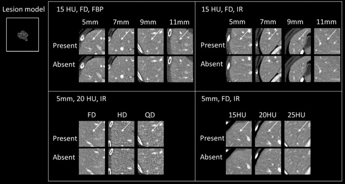
Example images of lesion‐present and lesion‐absent cases (only the middle image out of the five consecutive images for each trial is shown) across different experimental conditions. The inset image illustrates the middle slice (zoom reconstruction) of the base lesion model used in this study. Upper left: lesion size was varied across 5, 7, 9, and 11 mm, lesion contrast was 15 HU, computed tomography (CT) images were acquired at full routine radiation dose (FD) with the weighted filtered back projection. Upper right: the experimental condition was similar to that in upper left, except that CT images were reconstructed using iterative reconstruction (IR). Bottom left: lesion size was 5 mm, lesion contrast was 20 HU, CT images were acquired with IR, but radiation dose was varied across full, half and quarter of routine dose level (FD, HD, & QD, respectively). Bottom right: lesion size was 5 mm, CT images were acquired with IR at full radiation dose, but lesion contrast was varied across 15, 20, and 25 HU. The arrows indicate the lesion locations.
2.B.3. Data augmentation
To improve the performance of DL‐MO, we used several data augmentation strategies to augment the experimental trial images, including image conversion, cropping, z‐direction interpolation, and small angle rotation. Image conversion was used to convert the dynamic range of CT images to that of the natural images in ImageNet, while the other strategies were mainly used to increase the amount of training samples. These strategies were briefly introduced as follows. In image conversion, the original images were transformed to the grayscale of [0, 255] after applying an abdominal display window (WW/WL: 400/40 HU), that is, to make CT images more similar to the natural images in ImageNet. Specifically, the CT numbers were restricted to the dynamic range defined by the abdominal display window (i.e., [−160, 240] HU), and then were normalized to the range [0, 255]. The central three images of each VOI were retrieved to form a pseudo color image as the input of DL‐MO, by stacking the three images as RGB channels. This is because ResNet‐50 was pretrained to classify the natural images with RGB channels. Thus, the first and the last images of each VOI were excluded from the training of DL‐MO. Nevertheless, we expect such trivial adjustment will not downgrade DL‐MO performance, since the central three images already contained the most significant signal information. As for cropping, additional multisized VOIs were cropped out of each VOI. The size of these VOIs uniformly ranged from 7.4 × 7.4 mm2 to 52.0 × 52.0 mm2 in axial plane. These augmented VOIs were not resized to 224 × 224 pixels (i.e., the typical image size used in ImageNet), and thus, the dimension of the extracted CNN codes depended on the size of the input VOI. For instance, a VOI with 70 × 70 × 3 voxels (i.e., 52.0 × 52.0 × 9 mm3) would yield a CNN code with 5 × 5 × 256 features, at the 26th convolutional layer. So, zero padding was applied to each feature channel of the extracted CNN codes from smaller VOIs to ensure that all CNN codes had consistent dimension (i.e., 5 × 5 × 256 features per sample). In z‐direction interpolation, a voxel‐wise interpolation along z‐direction was used to generate more VOIs (still with 3 mm slice increment). For small angle rotation, each VOI was rotated by a random angle from a uniform distribution within the range of [−5.0°, 5.0°], and a “nearest neighbor” interpolation method was used to generate the rotated images, to avoid significantly altering image texture. Together, these data augmentation strategies generated 9, 424 additional lesion‐present and lesion‐absent trials for each experimental condition.
2.C. DL‐MO studies
We constructed 12 DL‐MOs separately to perform a two‐alternative forced choice detection (2AFC) task, that is, one DL‐MO for each experimental condition. The 26th convolutional layer of ResNet‐50 and the most significant 20 PLS components were used to build each DL‐MO. The configuration of the CNN layer and PLS components was empirically determined using a coarse grid search strategy in each experimental condition, that is, experimentally evaluating DL‐MO performance across different configurations. Note that the internal noise was excluded during grid search process. The impacts of different CNN layers and PLS components are demonstrated in Section 3.A. A resubstitution strategy38 was used to calculate DL‐MO test statistics, that is, the training dataset and the testing dataset were both generated out of the same set of CT images. A bootstrapping method was used to estimate the mean and the standard deviation of the test statistics. The bootstrapping was repeated for 200 times at each experimental condition. In each bootstrapping iteration, the training samples were randomly resampled (with replacement) from the augmented dataset, and the number of training samples was equal to that of the augmented dataset (i.e., 9424 samples). DL‐MO performance was also calibrated with the averaged HO performance at experimental condition #10, by adjusting the weighting factor α of the internal noise component (See Section 3.C.).
2.D. HO studies
Four medical physicists were recruited to perform the HO studies. Each reader performed the 2AFC detection task for the same 12 experimental conditions used in the DL‐MO study in three reading sessions, with four conditions at each session. For each trial, lesion‐present case and lesion‐absent case were displayed side by side with random placement, using the same graphical user interface as used in prior works8, 15 (Fig. 3). Furthermore, HOs were required to scroll through five images per VOI to identify the lesion‐present cases (i.e., multislice viewing mode). In each reading session, HOs were encouraged to take breaks to avoid fatigue, and they were also allowed to revisit any previous trials and modify their interpretation. The viewing parameters were fixed: all images were displayed with the soft tissue window (WW/WL: 400/40 HU); the viewing distance approximately 50 cm.
Figure 3.
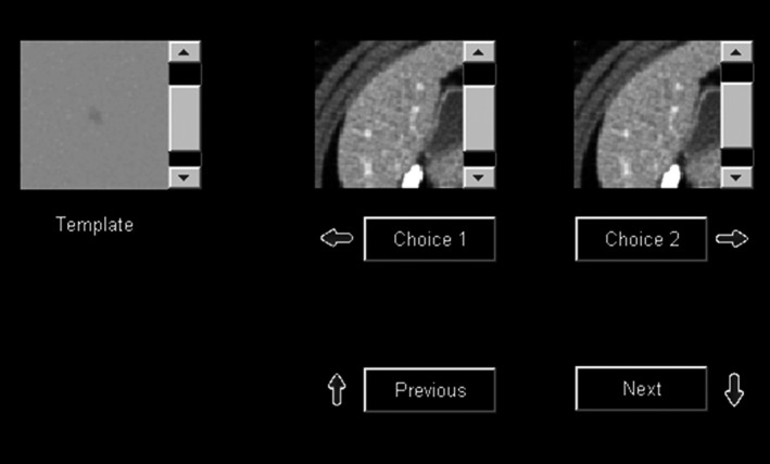
Graphical user interface that was used in human reader studies for the two‐alternative forced choice lesion detection task with multislice scrolling viewing mode.
2.E. Figure of merit and statistical analyses
For the DL‐MO study, the area under receiver operating characteristic curve (AUC_ROC) was used as the figure of merit (FOM) to represent the performance at each experimental condition. The ROC curve was generated by varying the decision threshold and compared with the test statistics of signal present and signal absent images. The mean and the standard deviation (STD) of AUC_ROC were calculated based on the 200 bootstrapping iterations. For the HO study, we used percent correct (PC) as the FOM to represent the HO performance in each 2AFC detection task. In each experimental condition, PC was calculated by dividing the number of correctly identified lesion‐present cases over the total number of trials. Note that AUC_ROC is considered to be equivalent to PC in 2AFC detection task38, 39 if the model observer response follows a normal distribution. Thus, the normality of DL‐MO test statistics was evaluated to verify the use of AUC_ROC as the FOM of DL‐MO in the 2AFC task. Specifically, we qualitatively tested the normality of λ 0 (excluding internal noise) separately for lesion‐present/absent images in each experimental condition, since the internal noise component had been formulated as a normal random variable. Finally, the strength of correlation and agreement between DL‐MO and HOs was evaluated across all experimental conditions, using Pearson's product moment correlation analysis and Bland–Altman plots.
3. Results
3.A. Grid search for optimal CNN layer and PLS components
An example of coarse grid search is shown in Fig. 4. The value of AUC_ROC was moved toward saturation, as the number of PLS components increased. This is because the feature variance was better represented by more PLS components. However, the use of a larger set of PLS components may result in a higher chance of overfitting the DL‐MO, so we intended to select the fewest PLS components that still yield a high performance. Furthermore, the 26th convolutional layer was able to achieve higher AUC_ROC with fewer PLS components, which suggested a higher feature transferability toward the target task T T . Therefore, we selected the 26th convolutional layer and the first 20 PLS components as the optimal configuration for building DL‐MO.
Figure 4.
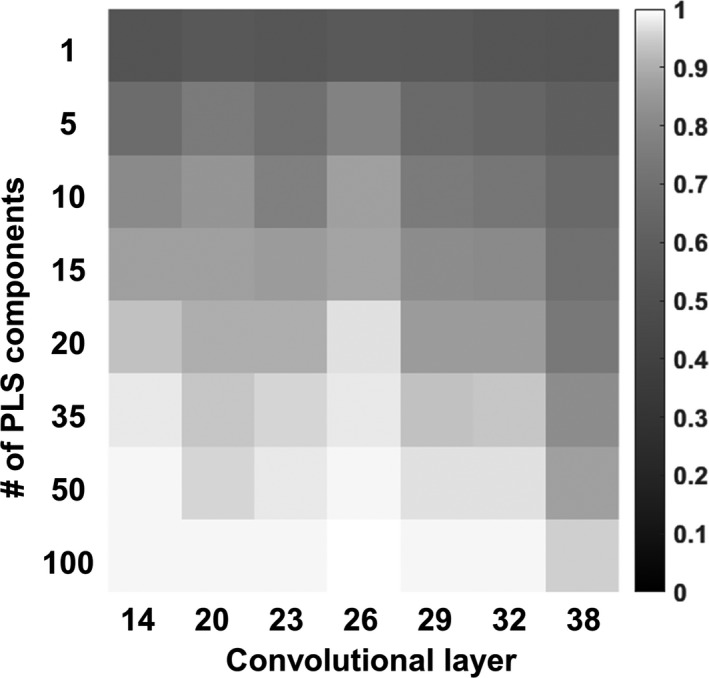
An example heatmap of the area under receiver operating characteristic curve (AUC_ROC; without internal noise, that is, α = 0) acquired from the coarse grid search at experimental condition #10, with varying configurations of convolutional layer and partial least square (PLS) components. These configurations involved the 14th to 38th convolutional layers in ResNet‐50, and the 1st to 100th PLS components. The value of AUC_ROC is represented by grayscale intensity.
Several examples of the CNN codes from ResNet‐50 are illustrated in Fig. 5. It is typically challenging for human readers to directly interpret these CNN codes from the deep layers. However, the difference between lesion‐present/absent CNN codes revealed the presence of the encoded structural information around the lesion location, that is, the central region of each lesion‐present image. This phenomenon has indicated the capability of ResNet‐50 in preserving the lesion‐relevant information.
Figure 5.

Examples of the convolutional neural network (CNN) codes and the corresponding absolute difference from a pair of lesion‐present/absent images, at the 26th convolutional layer of ResNet‐50. The inset computed tomography (CT) images (70 × 70 pixels) illustrate a pair of lesion‐present/absent examples from condition #1, and the arrow indicates the lesion location. These CNN codes corresponded to six randomly selected feature channels at the corresponding network layer. The images at each column correspond to the same convolutional filter channel. The display window of the difference images was narrowed down ([0, 0.4]) for the convenience of illustration.
Furthermore, some examples of the PLS components and regression coefficients (i.e., the template B) are illustrated in Fig. 6. As presented in Section 2.A.2, the PLS components were used to generate the template B that provided a set of weights to combine all features to form the test statistics λ 0. The features at the central region of the CNN codes (i.e., the lesion location) generally received stronger weights than those at the peripheral region. This finding indicated that the proposed model observer used the lesion‐relevant information and the surrounding patient anatomy to form the final test statistics.
Figure 6.
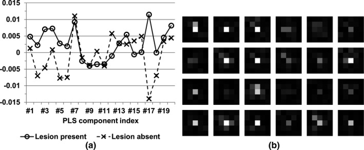
Examples of partial least square (PLS) components and regression coefficients (i.e., the template B), from the experimental condition #1. The corresponding convolutional neural network (CNN) codes were extracted from the 26th convolutional layer of ResNet‐50. (a) The most significant 20 PLS components from a pair of lesion‐present/absent images. (b) The PLS regression coefficients with respect to the randomly selected feature channels from the 26th convolutional layer of ResNet‐50 and were reshaped to match the spatial location of image features, for the convenience of illustration. The display window was [0, 0.06].
3.B. Normality of test statistics λ 0
The normality of the test statistics λ 0 was qualitatively evaluated using the normal probability plots.40 Briefly, the sorted samples of λ 0 (i.e., the y‐axis) were plotted against a theoretical normal distribution (i.e., the x‐axis) that was generated as the normal order statistics medians, and a straight line was fitted to the sample points to indicate the similarity to normality, that is, there existed a strong similarity if the majority of the sample points appeared along this line. As illustrated in Fig. 7, the statistical distribution of λ 0 well approximated normal distribution. Thus, it is reasonable to consider the AUC_ROC of DL‐MO as an equivalent FOM of the PC of HOs in the 2AFC task.
Figure 7.
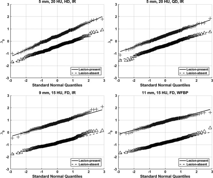
Examples of normal probability plots of test statistics λ 0 (without internal noise) for lesion‐present/absent cases in experimental conditions #10 (upper left), #9 (upper right), #7 (bottom left), and #8 (bottom right). The distribution of λ 0 approximated the normal distribution.
3.C. Internal noise calibration
The calibration was carried out on the experimental condition #10. Specifically, the value of the weighting factor α was increased from 0.1 to 5.5 with an increment of 0.01 per step. The resultant AUC_ROC of DL‐MO was compared with the averaged PC of HOs at the same condition to determine a proper value of α (Fig. 8). The value of α was determined to be 1.1, that is, the internal noise was 1.1 times of the noise of λ 0,bkg .
Figure 8.
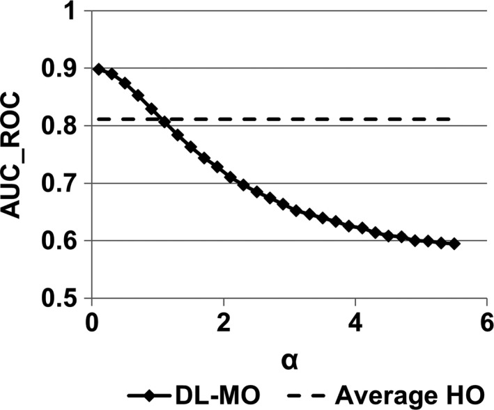
The weighting factor α was adjusted to calibrate deep learning‐based model observer (DL‐MO) performance to the averaged human observers (HOs) performance at the experimental condition #10, that is, lesion size was 5 mm, lesion contrast was 20 HU, radiation dose was half of routine dose level, and computed tomography images were reconstructed by iterative algorithm. The value of α was varied from 0.1 to 5.5 with a uniform interval of 0.1. Every second sample was plotted out for the convenience of illustration. The error bars indicate the standard deviation of DL‐MO performance. AUC_ROC denotes the area under the receiver operating characteristic curve.
3.D. Statistical analyses
The 12 experimental conditions were regrouped into four scenarios for convenience of comparing DL‐MO with HO (Fig. 9). The AUC_ROC of DL‐MO was comparable to the PC of HO in each condition. Pearson's correlation coefficient was 0.986 (with 95% CI [0.950, 0.996]). Bland–Altman plots indicated that there was no statistically significant discrepancy between DL‐MO and HO (Fig. 10). The bias between DL‐MO and HO was 0.25%. The upper and the lower limits of agreement were 4.00% (with 95% CI [1.90%, 6.11%]) and −3.51% (with 95% CI [−5.61%, −1.40%]), respectively.
Figure 9.
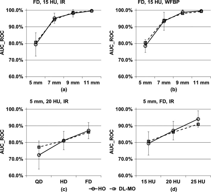
Comparison of deep learning‐based model observer (DL‐MO) and human observer (HO) in four scenarios. (a) Lesion size was varied across 5, 7, 9, and 11 mm, lesion contrast was 15 HU, computed tomography (CT) images were acquired with iterative reconstruction (IR) at full routine dose (FD). (b) Similar to the scenario in (a), but CT images were reconstructed with weighted filtered back projection (WFBP). (c) Lesion size was 5 mm, lesion contrast was 20 HU, CT images were reconstructed with IR across full, half, and quarter of routine radiation dose level (FD, HD & QD). (d) Lesion size was 5 mm, lesion contrast was varied across 15, 20, and 25 HU; CT images were acquired with IR at FD. The error bars indicate the standard deviation of the area under receiver operating characteristic curve (AUC_ROC).
Figure 10.
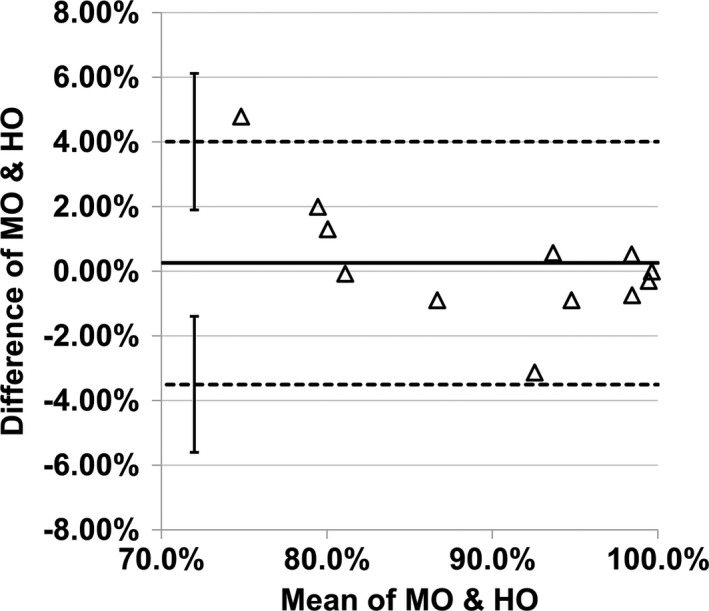
Bland–Altman plot of the difference of area under the receiver operating characteristic curve across all 12 experimental conditions. The two dashed lines denote the upper and the lower limits of agreement (LOA). The solid line denotes the bias. The error bars indicate the 95% confidence interval of LOA.
4. Discussion
In this study, we proposed a framework of DL‐MO that incorporated a state‐of‐the‐art deep CNN, PLS‐DA model, and an internal noise component. The comparison between the proposed DL‐MO and HOs was carried out over multiple experimental conditions with varying lesion attributes, radiation dose, and reconstruction types. We observed strong correlation and agreement between DL‐MO and the averaged HO performance.
The proposed DL‐MO framework was based on a fundamental hypothesis that there exists similarity between the state‐of‐the‐art CNN architectures and human visual system in object detection. This hypothesis was at least partially supported by several prior studies, which systematically investigated the correlation between CNN architectures and human neural response using carefully designed psychophysical experiments.41, 42, 43 Nonetheless, the corresponding degree of similarity varied a lot across different CNN architectures, which could be attributed to the different feature representation power of those CNNs. If using a different pretrained CNN architecture in the DL‐MO framework, the strength of the correlation and agreement with HOs may be altered. In this work, it is conjectured that the state‐of‐the‐art CNN architecture is more likely to be human‐like, due to the large feature representation power of these CNNs. The pretrained ResNet‐50 was used in this study, since it has demonstrated outstanding learning capacity in comparison with other networks in multiple challenging image classification and object detection tasks.27 It is possible that other state‐of‐the‐art CNN architecture may also work, but thus far, there is still a lack of theoretical guideline on what types of CNN architectures could be optimally correlated with HOs. The experimental validation similar to the current study is an effective way to select a proper architecture from the existing CNNs.
Besides the internal noise weighting factor α, DL‐MO has two additional free parameters, that is, the CNN layer used for feature extraction, and the number of PLS components used for building PLS‐DA model. These two parameters need to be properly determined to achieve reasonable DL‐MO performance in the target task T T . It is difficult to provide a theoretical prediction of the optimal configuration of CNN layer and PLS components, which is partially attributed to the extreme complexity of estimating the feature transferability of different layers. The feature transferability is negatively affected by two issues: the specificity of the CNN layers and the coadaption among neighboring layers.44 That being said, it is more likely for the features to transfer more poorly, when the following scenarios occur: source task T s is less similar to target task T T , the CNN layer has higher specialization toward T s , or the CNN was split at the coadapted layers. On the contrary, it is straightforward to experimentally validating the DL‐MO performance with respect to varying configurations of CNN layer and PLS components, that is, the coarse grid search strategy, to determine the appropriate CNN layer and PLS components that drive the DL‐MO to achieve high efficiency. Therefore, we used the coarse grid search strategy to empirically determine a proper selection of CNN layer and PLS components.
Conventional anthropomorphic MOs can estimate the effect of varying technical parameters on human perception for simple target structures and tasks using computer simulation or phantom images, while the proposed framework will provide a new MO, using deep learning techniques, which will enable the direct estimation of diagnostic performance using patient CT images for optimizing the CT protocols. Nevertheless, there exists some similarity between the DL‐MO framework and conventional anthropomorphic MOs. Take the channelized Hotelling observer (CHO) as an example: the pretrained CNN served as the fixed feature extractor, which may be viewed as a generic extension of the explicitly crafted channel filters (e.g., Gabor filters or dense difference of gaussian filters); the regression coefficient vector B (from the PLS‐DA model) was analogous to the template vector ω used in CHO; the internal noise component was directly extended from its counterpart in CHO. Furthermore, the AUC_ROC of DL‐MO and the PC of HOs were considered as equivalent FOMs as was done in the prior works8, 15 that involved CHO, since the DL‐MO response followed normal distribution. If DL‐MO response failed the normality test, the “template application”39 may be used as an alternative method to calculate PC as the FOM of DL‐MO. Briefly, the template would be directly applied to each pair of lesion‐present/absent cases, and the cases with larger test statistics would be typically considered as the lesion‐present ones. Thus, the PC of DL‐MO can be calculated across all experimental conditions. A systematic comparison between DL‐MO and the conventional MOs could be an interesting topic. However, there has been no agreement on how to apply conventional MOs to acquire sufficient statistics from the largely varying anatomical background. Thus, the comparison between DL‐MO and the conventional MOs is beyond the scope of the current study.
The application of data augmentation is not limited to the training of deep CNN models. In this work, the augmented data were used to improve the performance of PLS‐DA model, instead of fine‐tuning the pretrained ResNet‐50. The data augmentation was expected to induce more image feature variability and capture the underlying image statistics, which would be useful for improving the PLS‐DA model robustness and reducing overfitting. Similarly, previous studies have already used different types of data augmentation strategies with PLS and other classical machine learning techniques. For instance, noise augmentation was used to suppress the overfitting and improve PLS robustness against various types of random noise.45, 46 Elastic deformation and affine transformation were also effective in reducing overfitting and improving the accuracy of support vector machine and extreme learning machine.47
A large independent testing dataset was not prepared to evaluate the DL‐MO performance, as the data acquisition procedure was very resource‐intensive, especially for the collection of human reader performance. To complete this study with a comprehensive evaluation of DL‐MO performance, we present here a preliminary validation of the estimated DL‐MO generalization accuracy (i.e., the AUC on unseen data) with respect to the configuration of the 26th convolutional layer and the most significant 20 PLS components. Briefly, the estimated AUC from the resubstitution method was compared with the counterparts from two additional cross‐validation methods, including the tenfold cross‐validation (10f‐CV) and the bootstrap cross‐validation (BS‐CV) methods48 (Fig. 11). Note that the internal noise was excluded from the comparison. In the 10f‐CV method, the original experimental trials were randomly split into ten independent sub‐groups. Then, a single subgroup was selected as the validation dataset, while the other subgroups were used for training the DL‐MO. This process was repeated for ten times till each subgroup had been used once as the validation dataset. The averaged AUC across all ten validation datasets was used as the estimated DL‐MO generalization accuracy. In the BS‐CV method, the 10f‐CV was nested within the standard bootstrapping. The bootstrapping was repeated for 200 times with replacement (i.e., 200 resampled datasets), and the 10f‐CV was carried out on each resampled dataset to calculate the mean AUC from the validation datasets. Then, the mean AUC from the 200 resampled datasets was further averaged to estimate the DL‐MO generalization accuracy. In both methods, data augmentation was only applied to the training subsets to generate additional training samples, while each validation dataset had a small number of trials (n = 14 per condition). Of note, the 10f‐CV method tends to underestimate the generalization accuracy with a large variance, especially when using a small dataset.49 Compared to 10f‐CV, the BS‐CV method could achieve a more accurate estimation of the generalization accuracy with small samples, while suppressing the variance.48, 50 Considering the characteristics of these methods and the small size of the validation datasets, the three methods yielded comparable estimation of the generalization accuracy across all experimental conditions. Thus, we consider that there was no significant bias (i.e., overfitting) in the estimated DL‐MO performance. Note that the difference among the three methods shall further diminish as the sample size increases.
Figure 11.
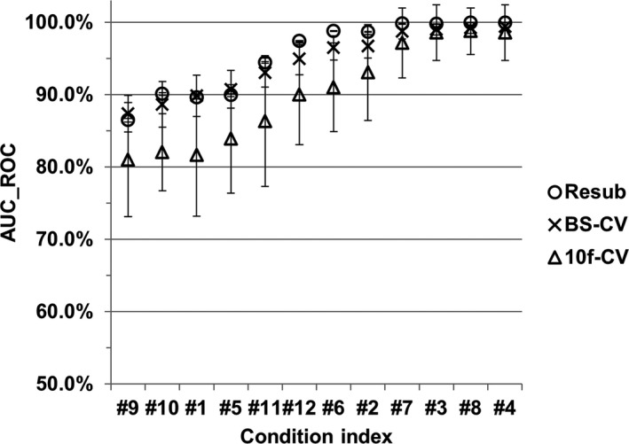
Comparison of the deep learning‐based model observer generalization accuracy that was estimated for the configuration of the 26th network layer and the most significant 20 PLS components, using the resubstitution (denoted as “Resub”), tenfold cross‐validation (denoted as “10f‐CV”), and bootstrap cross‐validation [denoted as bootstrap cross‐validation (“BS‐CV”)] methods, respectively, across all 12 experimental conditions. The generalization accuracy was gauged with the area under receiver operating characteristic curve (AUC_ROC). The condition indices were rearranged in the ascending order of the AUC_ROC value, for the convenience of illustration.
We acknowledge several limitations in the present work. First, we recruited nonradiologist readers (i.e., medical physicists) for HO study, and the number of readers may be limited. Second, although multislice scrolling was used as the viewing mode to mimic realistic tasks, the 2AFC lesion detection task is the simplest form of localization tasks, in which the lesion characteristics and locations were known exactly. Thus, the effects of anatomical background variability and tissue nonuniformity on HOs performance might be limited, compared with clinically realistic tasks. Third, we used only one base lesion model and one type of CT exam in data preparation. In clinical practice, radiologist readers are typically challenged to identify lesions with various imaging features. Meanwhile, it is desirable if the correlation between the proposed DL‐MO and HOs could be determined in multiple types of CT exams. Finally, the use of resubstitution method may result in positive bias in the FOM of DL‐MO, although such bias could decrease as the number of samples increases.38 We aim to address these limitations in the follow‐up study that employs radiologist readers and more realistic lesion localization tasks with patient abdominal/chest CT exams. Our preliminary results have suggested that a strong correlation between the proposed DL‐MO and HOs may be established in those challenging scenarios.51
The proposed DL‐MO framework could be readily applied for similar lesion detection tasks that involve different types of scanning protocols, lesion models, CT systems, and reconstruction algorithms, by retraining the DL‐MO using the images acquired from the new experimental conditions. In our ongoing work,51 we have observed the possibility of reusing the same configuration of CNN layer and PLS components for abdominal and chest CT exams with different base lesion models, whereas the weighting factor of the internal noise component needs readjustment. The further study would be necessary to validate these preliminary findings with additional types of CT exams and lesion models. If the retuning of the DL‐MO parameters (e.g., CNN layer and PLS components) is needed, one could still use the straightforward grid search strategy to find a proper configuration of DL‐MO parameters. Although the PLS has been successfully used in many data analytics tasks that involved small sample size with much larger feature dimensionality,52, 53, 54 the data augmentation strategies tend to be helpful to further enhance the model performance.
5. Conclusion
A framework of deep learning‐based model observer for task‐based image quality assessment was introduced. The performance predicted by DL‐MO was highly correlated with the HO performance in a 2AFC lesion detection task that involved realistic patient liver background and multislice viewing mode. This validation provided preliminary evidence for using DL‐MO to evaluate diagnostic image quality in realistic CT tasks.
Conflicts of Interest
Dr. Cynthia H McCollough is the recipient of a research grant from Siemens Healthcare. The other authors have no relevant conflicts of interest to disclose.
Acknowledgment
This study was sponsored by National Institute of Biomedical Imaging and Bioengineering of the National Institutes of Health under Award Numbers R01 EB017095 and U01 EB017185. The content is solely the responsibility of the authors and does not necessarily represent the official views of the National Institutes of Health.
References
- 1. Verdun FR, Racine D, Ott JG, et al. Image quality in CT: from physical measurements to model observers. Phys Med. 2015;31:823–843. [DOI] [PubMed] [Google Scholar]
- 2. McCollough CH, Yu L, Kofler JM, et al. Degradation of CT low‐contrast spatial resolution due to the use of iterative reconstruction and reduced dose levels. Radiology. 2015;276:499–506. [DOI] [PMC free article] [PubMed] [Google Scholar]
- 3. Kofler JM, Yu L, Leng S, et al. Assessment of low‐contrast resolution for the American College of Radiology Computed Tomographic Accreditation Program: what is the impact of iterative reconstruction? J Comput Assist Tomogr. 2015;39:619–623. [DOI] [PMC free article] [PubMed] [Google Scholar]
- 4. Christianson O, Chen JJ, Yang Z, et al. An improved index of image quality for task‐based performance of CT iterative reconstruction across three commercial implementations. Radiology. 2015;275:725–734. [DOI] [PubMed] [Google Scholar]
- 5. Barrett HH, Yao J, Rolland JP, Myers KJ. Model observers for assessment of image quality. Proc Natl Acad Sci USA. 1993;90:9758–9765. [DOI] [PMC free article] [PubMed] [Google Scholar]
- 6. ICRU Report 54 . International Commission on Radiation Units and Measurements (ICRU) Medical Imaging ‐ The Assessment of Image Quality; 1995.
- 7. Wunderlich A, Noo F. Image covariance and lesion detectability in direct fan‐beam x‐ray computed tomography. Phys Med Biol. 2008;53:2471–2493. [DOI] [PMC free article] [PubMed] [Google Scholar]
- 8. Yu L, Leng S, Chen L, Kofler JM, Carter RE, McCollough CH. Prediction of human observer performance in a 2‐alternative forced choice low‐contrast detection task using channelized Hotelling observer: impact of radiation dose and reconstruction algorithms. Med Phys. 2013;40:041908. [DOI] [PMC free article] [PubMed] [Google Scholar]
- 9. Leng S, Yu L, Zhang Y, Carter R, Toledano AY, McCollough CH. Correlation between model observer and human observer performance in CT imaging when lesion location is uncertain. Med Phys. 2013;40:081908. [DOI] [PMC free article] [PubMed] [Google Scholar]
- 10. Gang GJ, Stayman JW, Zbijewski W, Siewerdsen JH. Task‐based detectability in CT image reconstruction by filtered backprojection and penalized likelihood estimation. Med Phys. 2014;41:081902. [DOI] [PMC free article] [PubMed] [Google Scholar]
- 11. Samei E, Richard S. Assessment of the dose reduction potential of a model‐based iterative reconstruction algorithm using a task‐based performance metrology. Med Phys. 2015;42:314–323. [DOI] [PubMed] [Google Scholar]
- 12. Richard S, Li X, Yadava G, Samei E. Predictive models for observer performance in CT: applications in protocol optimization. Paper presented at: SPIE Medical Imaging; 2011.
- 13. Wilson JM, Christianson OI, Richard S, Samei E. A methodology for image quality evaluation of advanced CT systems. Med Phys. 2013;40:031908. [DOI] [PubMed] [Google Scholar]
- 14. Zhang Y, Leng S, Yu L, Carter RE, McCollough CH. Correlation between human and model observer performance for discrimination task in CT. Phys Med Biol. 2014;59:3389–3404. [DOI] [PMC free article] [PubMed] [Google Scholar]
- 15. Yu L, Chen B, Kofler JM, et al. Correlation between a 2D channelized Hotelling observer and human observers in a low‐contrast detection task with multi‐slice reading in CT. Med Phys. 2017;44:3990–3999. [DOI] [PMC free article] [PubMed] [Google Scholar]
- 16. Ba A, Eckstein MP, Racine D, et al. Anthropomorphic model observer performance in three‐dimensional detection task for low‐contrast computed tomography. J Med Imaging. 2016;3:011009. [DOI] [PMC free article] [PubMed] [Google Scholar]
- 17. Solomon J, Samei E. Correlation between human detection accuracy and observer model‐based image quality metrics in computed tomography. J Med Imaging. 2016;3:035506. [DOI] [PMC free article] [PubMed] [Google Scholar]
- 18. Abbey CK, Barrett HH. Human‐ and model‐observer performance in ramp‐spectrum noise: effects of regularization and object variability. J Opt Soc Am A. 2001;18:473–488. [DOI] [PMC free article] [PubMed] [Google Scholar]
- 19. Burgess AE. Evaluation of detection model performance in power‐law noise. Paper presented at: Medical Imaging 2001; 2001.
- 20. Kotre CJ. The effect of background structure on the detection of low contrast objects in mammography. Br J Radiol. 1998;71:1162–1167. [DOI] [PubMed] [Google Scholar]
- 21. Bochud FO, Valley JF, Verdun FR, Hessler C, Schnyder P. Estimation of the noisy component of anatomical backgrounds. Med Phys. 1999;26:1365–1370. [DOI] [PubMed] [Google Scholar]
- 22. Alnowami M, Mills G, Awis M, et al. A deep learning model observer for use in alterative forced choice virtual clinical trials. Paper presented at: SPIE Medical Imaging; 2018.
- 23. Massanes F, Brankov JG. Evaluation of CNN as anthropomorphic model observer. Paper presented at: SPIE Medical Imaging; 2017.
- 24. Kopp FK, Catalano M, Pfeiffer D, Fingerle AA, Rummeny EJ, Noel PB. CNN as model observer in a liver lesion detection task for x‐ray computed tomography: a phantom study. Med Phys. 2018;45:4439–4447. [DOI] [PubMed] [Google Scholar]
- 25. Zhou W, Anastasio MA. Learning the ideal observer for SKE detection tasks by use of convolutional neural networks (Cum Laude Poster Award). Paper presented at: SPIE Medical Imaging; 2018.
- 26. Baxter J. Theoretical models of learning to learn. In: Thrun S, Pratt L, eds. Learning to Learn. Boston, MA: Springer US; 1998:71–94. [Google Scholar]
- 27. He K, Zhang X, Ren S, Sun J. Deep residual learning for image recognition. Paper presented at: Proceedings of the IEEE conference on computer vision and pattern recognition; 2016.
- 28. Russakovsky O, Deng J, Su H, et al. ImageNet large scale visual recognition challenge. Int J Comput Vis (IJCV). 2015;115:211–252. [Google Scholar]
- 29. Ye JC, Han Y, Cha E. Deep convolutional framelets: a general deep learning framework for inverse problems. SIAM J Imaging Sci. 2018;11:991–1048. [Google Scholar]
- 30. Brereton RG, Lloyd GR. Partial least squares discriminant analysis: taking the magic away. J Chemom. 2014;28:213–225. [Google Scholar]
- 31. Palermo G, Piraino P, Zucht H‐D. Performance of PLS regression coefficients in selecting variables for each response of a multivariate PLS for omics‐type data. Adv Appl Bioinform Chem. 2009;2:57–70. [DOI] [PMC free article] [PubMed] [Google Scholar]
- 32. de Jong S. SIMPLS: an alternative approach to partial least squares regression. Chemometr Intell Lab Syst. 1993;18:251–263. [Google Scholar]
- 33. Rosipal R, Krämer N. Overview and recent advances in partial least squares. In: Saunders C, Grobelnik M, Gunn S, Shawe‐Taylor J, eds. Subspace, Latent Structure and Feature Selection. Berlin: Springer; 2006:34–51. [Google Scholar]
- 34. Yu L, Shiung M, Jondal D, McCollough CH. Development and validation of a practical lower‐dose‐simulation tool for optimizing computed tomography scan protocols. J Comput Assist Tomogr. 2012;36:477–487. [DOI] [PubMed] [Google Scholar]
- 35. Andrea F, Baiyu C, Zhoubo L, Lifeng Y, Cynthia M. Technical note: insertion of digital lesions in the projection domain for dual‐source, dual‐energy CT. Med Phys. 2017;44:1655–1660. [DOI] [PMC free article] [PubMed] [Google Scholar]
- 36. Stierstorfer K, Rauscher A, Boese J, Bruder H, Schaller S, Flohr T. Weighted FBP–a simple approximate 3D FBP algorithm for multislice spiral CT with good dose usage for arbitrary pitch. Phys Med Biol. 2004;49:2209–2218. [DOI] [PubMed] [Google Scholar]
- 37. Grant K, Raupach R. SAFIRE: Sinogram affirmed iterative reconstruction; 2012. http://www.usa.siemens.com/healthcare
- 38. Barrett HH, Myers KJ, Rathee S. Foundations of image science. Med Phys. 2004;31:953. [Google Scholar]
- 39. Beutel J, Kundel HL, Van Metter RL. Engineers SoP‐oI. In: Handbook of Medical Imaging. Bellingham, WA: Society of Photo Optical; 2000:619–621. [Google Scholar]
- 40. Chambers JM. Graphical methods for data analysis. Belmont, CA: Wadsworth International Group; 1983. [Google Scholar]
- 41. Kheradpisheh SR, Ghodrati M, Ganjtabesh M, Masquelier T. Deep networks can resemble human feed‐forward vision in invariant object recognition. Sci Rep. 2016;6:32672. [DOI] [PMC free article] [PubMed] [Google Scholar]
- 42. Güçlü U, van Gerven MAJ. Deep neural networks reveal a gradient in the complexity of neural representations across the ventral stream. J Neurosci. 2015;35:10005–10014. [DOI] [PMC free article] [PubMed] [Google Scholar]
- 43. Cadieu CF, Hong H, Yamins DLK, et al. Deep neural networks rival the representation of primate IT cortex for core visual object recognition. PLoS Comput Biol. 2014;10:e1003963. [DOI] [PMC free article] [PubMed] [Google Scholar]
- 44. Yosinski J, Clune J, Bengio Y, Lipson H. How transferable are features in deep neural networks? Proceedings of the 27th International Conference on Neural Information Processing Systems ‐ Volume 2; 2014, Montreal, Canada.
- 45. Mevik B‐H, Segtnan VH, Næs T. Ensemble methods and partial least squares regression. J Chemom. 2004;18:498–507. [Google Scholar]
- 46. Conlin AK, Martin EB, Morris AJ. Data augmentation: an alternative approach to the analysis of spectroscopic data. Chemometr Intell Lab Syst. 1998;44:161–173. [Google Scholar]
- 47. Wong SC, Gatt A, Stamatescu V, McDonnell MD. Understanding Data Augmentation for Classification: When to Warp? Paper presented at: 2016 International Conference on Digital Image Computing: Techniques and Applications (DICTA); 30 Nov.‐2 Dec. 2016; 2016.
- 48. Carroll RJ, Wang S, Fu WJ. Estimating misclassification error with small samples via bootstrap cross‐validation. Bioinformatics. 2005;21:1979–1986. [DOI] [PubMed] [Google Scholar]
- 49. Kohavi R. A study of cross‐validation and bootstrap for accuracy estimation and model selection. Proceedings of the 14th international joint conference on Artificial intelligence ‐ Volume 2; 1995, Montreal, Quebec, Canada.
- 50. Varma S, Simon R. Bias in error estimation when using cross‐validation for model selection. BMC Bioinform. 2006;7:91. [DOI] [PMC free article] [PubMed] [Google Scholar]
- 51. Gong H, Yu L, Leng S, McCullough C. Best in physics (Imaging): a deep learning based model observer for low‐contrast object detection task in x‐ray computed tomography. Paper presented at: Medical Physics; 2018.
- 52. Boulesteix AL, Strimmer K. Partial least squares: a versatile tool for the analysis of high‐dimensional genomic data. Brief Bioinform. 2007;8:32–44. [DOI] [PubMed] [Google Scholar]
- 53. Nguyen DV, Rocke DM. Tumor classification by partial least squares using microarray gene expression data. Bioinformatics. 2002;18:39–50. [DOI] [PubMed] [Google Scholar]
- 54. Carrascal LM, Galván I, Gordo O. Partial least squares regression as an alternative to current regression methods used in ecology. Oikos. 2009;118:681–690. [Google Scholar]


