Dynamic Hyper-Graph Inference Framework for Computer-Assisted Diagnosis of Neurodegenerative Diseases

Abstract

Hyper-graph techniques have been widely investigated in computer vision and medical imaging applications, showing superior performance for modeling complex subject-wise relationships and sufficient flexibility to deal with missing data from multi-modal neuroimaging data. Existing hyper-graph methods, however, are inadequate for two reasons. First, representations are generated only from the observed imaging data, a process that is completely independent of the subsequent data label inference/ classification step. Thus, hyper-graph results constructed in this way may not be consistent with phenotype data such as clinical labels or scores. More critically, it might generate sub-optimal predictions in relation to clinical labels/scores. Second, current hyper-graph inference methods rely on two sequential steps: 1) building the hyper-graph for each individual modality and then predicted latent labels for new subjects upon each constructed hyper-graph and 2) a voting procedure to incorporate inference results across different hyper-graphs. This approach, however, is limited by failing to consider the complex and complementary relationships of multi-modal imaging data with respect to hyper-graph inference procedure. To address these two issues, we propose a novel dynamic hyper-graph inference method supported by a semi-supervised framework. Our method iteratively estimates and adjusts the hyper-graph structures from multi-modal imaging data until consistency between the learned hyper-graph and the observed clinical labels and scores is achieved. This hyper-graph inference framework also eases the integration process of classification (identifying individuals having neurodegenerative disease) and regression (predicting the clinical scores) within the same framework. The experimental results on identifying mild cognition impairment (MCI) subjects and the fine grained recognition of MCI progression stages show improved performance using our proposed hyper-graph inference method compared with conventional methods.

1. INTRODUCTION

THE morphological patterns from neuroimaging data, either structural (e.g., MRI) or functional image (e.g., PET/SPECT) are highly correlated with progression of the neurodegenerative disorder, such as Alzheimer’s disease (AD) [1]–[6]. Due to large inter-subject variation and complex disease pathology, however, it is very challenging to design an imaging-based diagnosis system that can identify individual patient or high-risk subjects with high sensitivity and specificity. As different imaging modalities show complementary information, many state-of-the-art machine-learning approaches have been proposed to improve the diagnosis accuracy using multi-modal information [2], [6]–[9]. For example, multitask learning by ensemble SVM and SVR are used for AD and Mild Cognitive Impairment (MCI) classification and regression in [10]. A Deep Boltzmann machine is used to fuse multi-modal imaging data into a high-level representation for classification [11]. Although the above supervised learning approaches have shown promising results for integrating multi-modal imaging information for disease diagnosis, their accuracy and generalizability are restricted by the limited number of labelled training samples. To address this problem, semi-supervised learning approaches are explored as an alternative solution that uses both unlabeled and labeled data to train the diagnostic model [6], [12]–[14].

The second challenge is how to design a model to represent heterogeneous distributed data. A classic SVM and SVR based model (even with kernel) usually learns a general model on the whole dataset and assumes it can fit different testing subjects well. However, this assumption does not hold for heterogeneous distributed data. Personalized SVM and SVR model are proposed by Zhu et al., [37] in order to address the heterogeneity problem by reweighting training data to reveal the latent data distribution of different testing subject. However, this method requires multiple images from each testing person to learn the training data reweighting vector; its application is thus restricted by availability of longitudinal data. Graph-based models naturally model the relevance of training samples to testing sample by the edge structure. The weighted edges share similar idea of personalized diagnosis model. The training samples are weighted by edges such that the edges from training data to testing data represents their correlation (similarity).

Furthermore, clinical data shows complicated subject-to-subject relationships as, one subject might have connections to multiple subjects via different modalities. However, one-to-one edge setting in a simple graph is unable to model such complex relationships. Hyper-graph uses hyper-edge to represent multiple-to-multiple relationships and . thus, is more suitable for modeling the complicated clinical data from multiple modalities [15]. Hyper-graph has been successfully applied to various medical imaging areas including image segmentation [16] and classification [9], [17]. Recent work uses hypergraph to combine multi-modal neuroimaging information for identifying MCI subjects [9]. However, current hypergraph inference methods have the following two limitations. First, current approaches are built upon the assumption of strong correlation between imaging data and clinical labels. Hyper-graph is usually constructed using imaging data only, which is completely independent of the subsequent label inference. More critically, these hyper-graphs are not validated for label prediction on the training data (known labels). Due to the possible noisy and redundant patterns in the imaging features, the learned hyper-graph might be sub-optimal for the ultimate goal of label prediction. This, un-validated hyper-graph poses a high risk of misguiding the labels prediction on testing subject. Second, it is common to build multiple hyper-graphs, one for each modality independently, in multi-modal inference applications. For example, there are two hypergraphs constructed separately from morphological features extracted from MR and PET images in [9], as shown by blue and purple solid ellipses in the blue dash box of Fig. 1. The final classification result is a linear combination of label likelihood scores from different hyper-graphs. The multi-modal information is only used in fusing labels, which ignores the complex relationship between different modalities in the entire hyper-graph learning process.

Fig. 1.

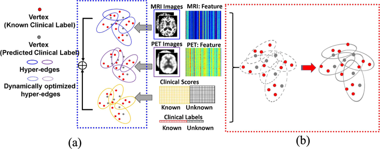
Illustration of conventional hyper-graph learning and our dynamic hyper-graph learning framework in computer-assisted diagnosis using multi-modal imaging data. (a) Independent hyper-graph construction. (b) Dynamic hypergraph learning for classification and regression.

To address these issues, we present a novel dynamic hyper-graph inference framework for multi-modal diagnosis of neurodegenerative disorders. Instead of constructing multiple hyper-graphs for different modal imaging data separately, we propose to generate a unified dynamic hyper-graph for all modalities regardless of the distinct imaging patterns across different modalities. Furthermore, both the imaging data and clinical labels on the training data are employed to learn the hyper graph, as shown in the red dash box of Fig. 1. Thus, the constructed hyper-graph is automatically validated on the training data for label predictions. Specifically, we alternatively estimate and refine the subject-wise relationship from multi-modal neuroimaging data until the learned hyper-graph representation satisfies the following criteria: (1) largely consistent with the subject-wise relation-ship measured by the observed multi-modal imaging data, and (2) optimally aligned with the clinical labels on the training dataset by minimizing the difference between the estimated labels and observed clinical labels.

Clinical phenotype data such as the MMSE and CDR scores in AD diagnosis are widely used in current learning based diagnostic methods because they have a higher correlation with clinical labels than imaging data [10], [18]. To that end, we further extend our hyper-graph inference framework to integrate both classification (identifying individuals with dis-eases) and regression (predicting the clinical scores). We apply our proposed hyper-graph based diagnostic method to identify MCI subjects and classify MCI subjects at different stages of progression. The experimental results demonstrate that our method outperforms conventional hyper-graph methods, rendering a 1.8% increase in discriminating MCI subjects from NC and AD cohorts, and a 3.1% increase in fine grained recognition on MCI sub-types, respectively.

II. METHOD

We will first briefly review the standard hyper-graph learning techniques and then introduce our dynamic hyper-graph learning framework, which integrates the classification and regression task.

A. Conventional Hyper-Graph Learning Model

1). Conventional Hyper-Graph Learning for Single Modality:

Following the definition of hyper-graph in [15], a hyper-graph is denoted as $\mathcal{G}$ = (V , E), where V = {v} is the vertex set and E = {e} is the hyper-edge set. Given N subjects with morphological features X = {x₁, . . . , x_N }, we first compute the N × N affinity matrix A, where each element a_ij measures the similarity between subject I_i and I_j (i, j = 1, . . . , N). Then, we construct the incidence matrix $H\left(H\in {\mathcal{R}}^{\left|V\right|\times \left|E\right|}\right)$ to encode the hyper-edge as follows. Each vertex v is allowed to establish multiple hyper-edges where each hyper-edge characterizes the similarity between underlying v and all other vertexes. For efficiency, the subject-to-subject relationship is binarized into a bit array (‘0’ stands for non-connected and ‘1’ stands for connected in the underlying hyper-edge) and further becomes one column vector in H . Note, a threshold ξ is required in binarization. As we will explain later, we use cross validation to determine the value of ξ in our experiments. Two diagonal matrices $D_v\in {\mathcal{R}}^{\left|V\right|\times \left|V\right|}$ and $D_e\in {\mathcal{R}}^{\left|E\right|\times \left|E\right|}$ can be calculated to represent the vertex degrees and hyper-edge degrees from the incidence matrix H as:

$${\mathbf{D}}_v\left(v,v\right)={\sum }_{e\in E}H\left(v,e\right),\hspace{1em}{\mathbf{D}}_e\left(e,e\right)={\sum }_{v\in V}H\left(v,e\right).$$ (1)

After that, the Laplacian matrix L of the hyper-graph can be computed as:

$$\mathit{L}=\mathit{I}-{\mathit{D}}_v^{-\frac{1}{2}}\mathit{H}{\mathit{D}}_e^{-1}{\mathit{H}}^T{D}_v^{-\frac{1}{2}}$$ (2)

where I is the |V|×|V| identity matrix. Note, we assume the hyper-edges have equal weight, for simplicity. Suppose N subjects consist of P training subjects with known clinical labels Yp =[y₁,...,y_P]and Q unseen testing subjects (N = P + Q). The goal of conventional hypergraph learning is to estimate the label probabilities for testing subjects by:

$$\arg \underset{\mathit{F}Q}{\min }tr\left({\mathit{F}}^T\mathit{L}\mathit{F}\right),$$ (3)

where F =[ F_P, F_Q] is the probability vector for all N subjects with the first P elements forming the probability vector F_P for P training subjects and the last Q elements forming the probability vector F_Q for Q testing subjects. Eq. 3 can be solved efficiently using Augmented Lagrange Methods (ALMs) [19].

The intuition behind hyper-graph learning is illustrated in the left panel of Fig. 2. The hyper-graph is fixed once built from the observed morphological features X, and then the latent labels on the testing subjects are determined, based on the encoded data representation in the hyper-graph, with respect to the neighboring training subjects with known labels. The prior knowledge of labels Y_P is not used to guide the learning of data representation.

Fig. 2.

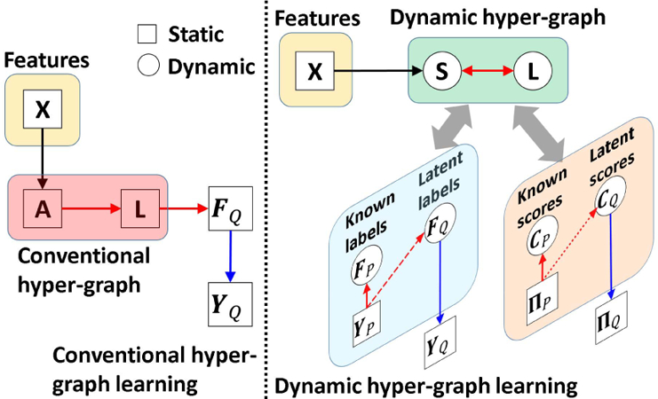
Comparison of conventional hyper-graph learning and our dynamic hyper-graph learning framework.

2). Extend to Multi-Modal Scenario:

In order to apply hypergraph to multi-modal imaging data, Gao et al. [9] proposed to combine multiple hyper-graph models using a linear model and estimate the unknown data labels on the combined multiple hyper-graphs. Suppose there are M set of morphological features {X^m|m = 1,...,M}, M hyper-graphs are constructed. A weighting vector α = [α_m]m=1,...,M is learned to measure the contribution of each modality. Similarly, the labels are propagated on the combined hyper-graph by solving:

$$\arg \underset{\alpha ,{\mathit{F}}_Q}{\min }tr\left[{\mathbf{F}}^T\left({\sum }_{m=1}^M{\alpha }_m{\mathit{L}}_m\right)\mathit{F}\right],\hspace{1em}s.t.\hspace{0.33em}\hspace{0.33em}{\sum }_{m=1}^M{\alpha }_m=1.$$

B. Dynamic Hyper-Graph Inference Framework

We propose an integrated method to solve the hyper-graph construction and label propagation/classification problems simultaneously. To do so, we estimate a hidden subject-wise affinity matrix S behind the observed multi-modal data, where s_ij represent the learned similarity between subject I_i and I_j , regardless of training or testing subjects. We optimize S towards two criteria: (1) imaging feature similarity: each s_ij should reflect the similarity between observed features $x_i^m$ and $x_j^m$ across all modalities; (2) clinical label similarity: s_ij should also be consistent to the label correlation between subject I_i and I_j if clinical labels available.

To cast the optimization of S into a well-posed problem, we further introduce the three constraints: (1) graph regularization term: Given S, we can construct the hyper-graph as well as the Laplacian matrix L. We require the estimated probability vector F agree with the data representation encoded in hyper-graph Laplacian matrix L by minimizing the hyper-graph regularization term [15] tr(FL^T F). (2) cross-validation constraint. Since the clinical labels Y_P are known for the training subjects, we requite the estimated probability vector F_P should have as less difference to Y_P as possible. (3) Frobenius norm: To avoid the trivial solution, we apply l₂-norm to S and the weighting vector α to constrain the energy. After integrating above similarity terms, clinical label validation terms and regularization terms, the energy function of our dynamic hyper-graph is:

$$\begin{gathered} \arg \underset{\mathit{S},\mathit{L},\alpha ,{\mathit{F}}_Q}{\min }\frac{1}{2}\sum _{i,j=1}^N\left(\sum _{m=1}^M{\alpha }_m{‖x_i^m-x_j^m‖}_2^2{s}_{ij} \\ +\beta {‖f_i-f_j‖}_2^2{s}_{ij}\right)+\gamma \cdot tr\left({\mathit{F}}^T\mathit{L}\mathit{F}\right)+{‖S‖}_2^2+{‖\alpha ‖}_2^2, \\ s.t.\left\{\begin{array}{l}{\mathit{F}}_P={\mathbf{Y}}_P\\ {\sum }_{m=1}^M{\alpha }_m=1,{\alpha }_m>0,{\sum }_{j=1}^N{s}_{ij}=1,s_{ij}>0\end{array}\right. \end{gathered}$$ (5)

where β and γ are used to balance the strength of label similarity term and hyper-graph regularization term, respectively.

The improvement of our dynamic hyper-graph learning over the conventional methods is illustrated in the right panel of Fig. 2. First, we allow using phenotype data to guide the optimization of hyper-graph construction. As we will explain the optimization procedure in section II.D, we seek for the intrinsic affinity matrix S which produce less dissimilarity between the known clinical labels Y_P and estimated likelihood F_P on the training subjects (indicated by the red dash arrows in Fig. 2). Since the hyper-graph $\mathcal{G}$ is built upon S, the optimized hyper-graph is more related to the eventual goal of classification. Second, we gradually refine the optimization of S by alternatively validating the classification performance on the training subjects and updating S. Thus, our dynamic hyper-graph learning framework can correct possible sub-optimal estimations in an iterative manner. We further extend current hyper-graph model from classification to regression task. The regression model and related parameters are described in Section C.

C. Joint Classification and Regression in Dynamic Hyper-Graph Inference Framework

Since convergent evidence shows clinical scores such as ADAS-COG [20] (Alzheimer’s Disease Assessment Scale-Cognitive Subscale) and MMSE [21] (mini mental state examination) in AD diagnosis, are very informative to monitor the progression of the neuro-disease in clinic routine practice, we further extend our dynamic hyper-graph inference framework to integrate both diagnosis labels the clinical scores, which eventually falls into a joint classification and regression scenario.

Specifically, let $\Pi \left(\Pi \in {\mathcal{R}}^{N\times D}\right)$ denote the matrix of estimated clinical scores, where each row π _i denotes a vector of D scores for each subject I_i . Without loss of generality, the first P subjects in Π are considered as training subjects with the known scores Π_P and the last Q subjects are testing subjects which need to estimate the scores Π_Q , i.e., Π = [Π_P , Π_Q ]. Using the same order of index, the N × D matrix C= [C_P , C_Q ] denotes the estimated clinical scores after hyper-graph learning. Following the concept of label propagation along the data representation via hyper-graph, we estimate the subject-specific weighing vector w_i (a column vector with N elements) which can restore the scores by using the linear combination of scores on other subjects, i.e., $c_i=w_i^{T}C$. Meanwhile, we require the estimated scores C_P on training subjects to be as close to the ground truth scores Π_P as possible.

$$\begin{gathered} \arg \underset{S,\mathbf{L},\alpha ,{\mathit{F}}_Q,C_Q,W}{\min }\frac{1}{2}{\sum }_{i,j=1}^N\left({\sum }_{m=1}^M{\alpha }_m{‖{\mathit{x}}_{\mathit{i}}^{\mathit{m}}-{\mathit{x}}_{\mathit{j}}^{\mathit{m}}‖}_2^2{s}_{ij}\right.\hspace{1em}\hspace{0.33em}\hspace{0.33em}\hspace{0.33em}\hspace{0.33em} \\ \left.+\beta {‖{\mathit{f}}_i-{\mathit{f}}_j‖}_2^2{s}_{ij}+\delta {‖{\mathit{c}}_i-{\mathit{c}}_j‖}_2^2{s}_{ij}\right)\hspace{1em}\hspace{0.33em}\hspace{0.33em}\hspace{0.33em}\hspace{0.33em} \\ +\gamma \cdot tr\left({\mathit{F}}^T\mathit{L}\mathit{F}\right)+{‖\mathit{S}‖}_2^2+{‖\alpha ‖}_2^2, \\ s.t.\left\{\begin{array}{ccc}{\mathit{F}}_P={\mathit{Y}}_P,& {\mathit{C}}_P={\Pi }_P,& \mathit{C}={\mathit{W}}^T\mathit{C}\\ {\sum }_{m=1}^M{\alpha }_m=1,& {\alpha }_m>0,& {\sum }_{j=1}^N{s}_{ij}=1,\hspace{0.33em}{s}_{ij}>0\end{array}\right. \end{gathered}$$ (6)

where W = [w_i ]_i=1,...,N is a N × N matrix and δ is a scalar to control the impact of regression error in Eq. 6. As shown in the right of Fig. 2, our dynamic hyper-graph will learn the data representation which considering both the image feature similarity on all subjects and label/score similarity on training subjects.

D. Optimization

Since the energy function in Eq. 6 is convex, we can efficiently obtain F _Q and C _Q using ALMs [19]. Specifically, we introduce several Lagrange multipliers to remove the equality constraints as:

$$\begin{gathered} \arg \underset{S,\mathbf{L},\alpha ,{\mathit{F}}_Q,C_Q,W}{\min }\frac{1}{2}{\sum }_{i,j=1}^N\left({\sum }_{m=1}^M{\alpha }_m{‖x_i^m-x_j^m‖}_2^2{s}_{ij}\right.\hspace{1em}\hspace{1em} \\ \left.+\beta {‖{\mathit{F}}_i-{\mathit{F}}_j‖}_2^2{s}_{ij}+\delta {‖c_i-c_j‖}_2^2{s}_{ij}\right)\hspace{1em}\hspace{1em} \\ +\gamma \cdot tr\left({\mathit{F}}^T\mathit{L}\mathit{F}\right)+{‖S‖}_2^2+{‖\alpha ‖}_2^2\hspace{1em}\hspace{1em} \\ +\frac{{\mu }_{\mathit{F}}}{\mathbf{2}}{‖{\mathit{F}}_Q-Y_Q‖}_2^2+tr\left({\Lambda }_{\mathit{F}}\left({\mathit{F}}_Q-Y_Q\right)\right)\hspace{1em}\hspace{1em} \\ +\frac{{\mu }_c}{\mathbf{2}}{‖{\mathit{C}}_Q-{\Pi }_Q‖}_2^2+tr\left({\Lambda }_c\left({\mathit{C}}_Q-{\Pi }_Q\right)\right)\hspace{1em}\hspace{1em} \\ +\frac{{\mu }_w}{\mathbf{2}}{‖{\mathit{W}}^T\mathit{C}-\mathit{C}‖}_2^2+tr\left({\Lambda }_w\left({\mathit{W}}^T\mathit{C}-\mathit{C}\right)\right), \\ s.t.{\sum }_{m=1}^M{\alpha }_m=1,{\alpha }_m>0,\hspace{1em}{\sum }_{j=1}^N{s}_{ij}=1,s_{ij}>0 \end{gathered}$$ (7)

Where Λ_f , Λ_c , and Λ_w are standard Lagrange multipliers and _μf , μ_c, and μ_w are the penalty parameters in ALMs. After that, we can alternately estimate S, F _Q , C _Q , α, and W via the following simple sub-tasks where we optimize one viable at a time by fixing the other variables:

• Sub-task 1: Estimate affinity matrix S based on latest F and C .

$$\begin{gathered} \arg \underset{S}{\min }\frac{1}{2}{\sum }_{i,j=1}^N\left({\sum }_{m=1}^M{\alpha }_m{‖x_i^m-x_j^m‖}_2^2{s}_{ij}\right. \\ \hspace{1em}\hspace{1em}\hspace{1em}\hspace{0.33em}\left.+\beta {‖f_i-f_j‖}_2^2{s}_{ij}+\delta {‖{\mathit{c}}_i-{\mathit{c}}_j‖}_2^2{s}_{ij}\right)+{‖\mathit{S}‖}_2^2 \end{gathered}$$ (8)

• Sub-task 2: Estimate latent labels F _Q based on latest hyper-graph.

$$\begin{gathered} \arg \underset{{\mathit{F}}_Q}{\min }\frac{1}{2}{\sum }_{i,j=1}^N\left(\beta {‖f_i-f_j‖}_2^2{s}_{ij}\right)+\gamma \cdot tr\left({\mathit{F}}^T\mathit{L}\mathit{F}\right) \\ \hspace{1em}\hspace{1em}\hspace{1em}\hspace{1em}+tr\left({\Lambda }_{\mathit{F}}\left({\mathit{F}}_Q-{\mathit{Y}}_Q\right)\right)+\frac{{\mu }_c}{\mathit{2}}{‖{\mathit{C}}_Q-{\Pi }_Q‖}_2^2 \end{gathered}$$ (9)

• Sub-task 3: Estimate latent scores C _Q based on latest hyper-graph.

$$\begin{gathered} \arg \underset{{\mathit{C}}_Q}{\min }\frac{1}{2}{\sum }_{i,j=1}^N\left(\delta {‖{\mathit{c}}_i-{\mathit{c}}_j‖}_2^2{s}_{ij}\right)+\frac{{\mu }_c}{2}{‖{\mathit{C}}_Q-{\mathit{\Pi }}_Q‖}_2^2 \\ \hspace{1em}+tr\left({\mathit{\Lambda }}_c\left({\mathit{C}}_Q-{\mathit{\Pi }}_Q\right)\right)+\frac{{\mu }_w}{\mathit{2}}{‖{\mathit{W}}^T\mathit{C}-\mathit{C}‖}_2^2 \\ \hspace{1em}+tr\left({\mathit{\Lambda }}_w\left({\mathit{W}}^T\mathit{C}-\mathit{C}\right)\right) \end{gathered}$$ (10)

• Sub-task 4: Estimate the weight α_m for each modality.

$$\arg \underset{\alpha }{\min }\frac{1}{2}{\sum }_{i,j=1}^N\left({\sum }_{m=1}^M{\alpha }_m{‖x_i^m-x_j^m‖}_2^2{s}_{ij}\right)+{‖\alpha ‖}_2^2$$ (11)

• Sub-task 5: Estimate the regression matrix W based on latest scores C .

$$\arg \underset{\mathit{W}}{\min }\frac{{\mu }_w}{\mathbf{2}}{‖{\mathit{W}}^T\mathit{C}-C‖}_2^2+tr\left({\mathbf{\Lambda }}_w\left({\mathit{W}}^T\mathit{C}-\mathit{C}\right)\right)$$ (12)

Note, Eq. 8 and Eq. 11 are quadratic problems with similar linear inequality constraints, which can be efficiently solved using Karush Kuhn Tunker (KKT) approach [22]. Eq. 9–10 and 12 are standard unconstrained quadratic problems that can be efficiently solved by gradient search with respect to C _Q , F _Q , and W . All sub-problems are iteratively solved until the overall objective function converges. The Lagrange multiplier parameters are updated using following equations:

$$\left\{\begin{array}{l}{\mathbf{\Lambda }}_f={\mathbf{\Lambda }}_f+{\mu }_f\left({\mathit{F}}_Q-{\mathit{Y}}_Q\right)\hspace{1em}{\mu }_f=\rho \cdot {\mu }_f\hfill \\ {\mathbf{\Lambda }}_c={\mathbf{\Lambda }}_c+{\mu }_c\left({\mathit{C}}_Q\mathbf{-}{\Pi }_Q\right)\hspace{1em}{\mu }_c=\rho \cdot {\mu }_c\hfill \\ {\mathbf{\Lambda }}_w={\mathbf{\Lambda }}_w+{\mu }_w\left({\mathit{W}}^T\mathit{C}-\mathit{C}\right)\hspace{1em}{\mu }_w=\rho \cdot {\mu }_w\hfill \end{array}\right.$$ (13)

where ρ is the learning step parameter to increase the equality constraint penalty during the iterations. We fix ρ = 1.1 in our experiments.

E. Discussion

1). Further Improvement: Integration With Metric Learning Technique:

Our proposed dynamic hyper-graph learning framework and the widely used metric learning technique [23], [24] are similar in that both focus on latent subject-to-subject relationships, instead of the subject-wise similarity based on the observed data. Metric learning technique is compatible with many machine learning models, including our proposed dynamic hyper-graph model. To do so, we use Θ^m denote the to-be-learned projection matrix which can map each data $x_i^m$ to a new space and then calculate the distance basded on the learned metric. Following the standard metric learning approach in [23], we can slightly modify our energy function in Eq. 6 as:

$$\begin{gathered} \arg \underset{\mathit{S},\mathit{L},\alpha ,{\mathit{F}}_Q,{\mathit{C}}_Q,\mathit{W}}{\min }\frac{1}{2}{\sum }_{i,j=1}^N\left({\sum }_{m=1}^M{\alpha }_m{‖{\Theta }^m{x}_i^m-{\Theta }^m{x}_j^m‖}_2^2{s}_{ij}\right. \\ \hspace{0.33em}\hspace{0.33em}\left.+\beta {‖f_i-f_j‖}_2^2{s}_{ij}+\delta {‖{\mathit{c}}_i-{\mathit{c}}_j‖}_2^2{s}_{ij}\right)+\gamma \cdot tr\left({\mathit{F}}^T\mathit{L}\mathit{F}\right) \\ \hspace{0.33em}\hspace{0.33em}+{‖\mathit{S}‖}_2^2+{‖\mathit{\alpha }‖}_2^2+{\sum }_{m=1}^M{‖{\Theta }^m‖}_2^2, \end{gathered}$$ (14)

where the projection matrix Θ^m for each modality is constrained by l₂ norm.

2 ). Further Extension Handle the Missing Data Problem in Diagnosis:

Due to poor data quality and subject dropout, the problem of missing data is a big obstacle to conquer in multi-modal studies. Rather than completing the missing data based on statistical correlations [25], [26] and train the learning model consequently, our hyper-graph based model is straight forward to deal with the missing data issue in the learning process (Eq. 5 and Eq. 6). Following the suggestion in [27], we can replace thel₂-normwith l₁ norm on S, to make our model more robust to missing data.

III. EXPERIMENTS

We apply our method for computer-assisted diagnosis of AD, which is the most common neuro-degenerative dementia featuring memory loss, other cognitive deficits, and altered behavior [4], [28], [29]. A high-risk stage of possible incipient AD is called MCI, which is characterized by measurable cognitive changes in the absence of clinically significant functional impairment [30]–[32]. Convergent evidence shows that many MCI subjects are in a prodromal stage of AD. Although some subjects can persist in the MCI stage for a long time, referred to as MCI Non-Converters (MCI-NC), other MCI subjects who eventually develop AD are referred to as MCI Converters (MCI-C). Thus, identifying the heterogeneous subtypes such as AD, MCI-C, MCI-NC and predicting the clinical score of potential AD patients is of high impact in clinical practice. In the following, we evaluate the performance of hyper-graph learning framework in identifying the heterogeneous subtypes of AD and predicting the clinical score using multiple modality imaging data.

A. Image Processing

In our experiments, we use the baseline MRI, PET images from the Alzheimer’s Disease Neuroimaging Initiative (ADNI) dataset (www.adni-info.org) including 93 AD subjects and 101 NC (Normal Control). In addition, 118 MCI subjects are selected which include 55 MCI-C and 63 MCI-NC subjects. The ADAS-COG and MMSE scores are available in all selected subjects. For each subject, we first register their MR and PET images using the linear registration tool in FSL package (http://fsl.fmrib.ox.ac.uk/fsl/fslwiki/). Then, we apply skull removal [33], bias correction [34], and intensity normalization [35] and tissue segmentation using FAST in FSL package. After that, we obtain the parcellation of 90 anatomical structures by warping the AAL template (with manually labeled regions) to the underlying subject. Finally, the volume percentile of gray matter and the average intensity of PET image in each ROI (region of interest) are used as the morphological features.

B. Experiment Settings

1). Experiment Setup:

We have evaluated the performance of our dynamic hyper-graph learning framework on two binary classification problems (MCI/NC and MCI-C/MCI-NC classification) and two multiple class classification problems (3-class AD/MCI/NC classification and 4-class AD/MCI-C/ MCI-NC/NC classification). We use a 10-fold cross validation strategy in performance evaluation. Note, we do not use leave-one-out cross validation because it will produce unreliable and biased results as reported in [36]. Specifically, we randomly partition the subjects into 10 non-overlapping folds with approximately equal size subsets. Each time one fold is used for testing and all subsets in other folds are considered as training subjects. The optimal parameters are learned by grid search strategy in the training set using five-fold inner cross-validation. The search range for parametersβ, γ and δ is [10⁻³,10³]. We repeat such cross validation procedure for 10 times and report the overall score of classification/regression performance. Three measures are used for classification performance evaluation: accuracy (ACC), sensitivity (SEN) and specificity (SPEC). The correlation coefficients (CC) and root mean square error (RMSE) are used to evaluate the regression accuracy.

2). Counterpart Methods:

We choose the recent work of hyper-graph classification in [9] as the representative method of conventional hyper-graph learning approaches. Since the hyper-graph is fixed after construction, we call the method in [9] as static hyper-graph in the experiment. As SVM is popular in computer assisted diagnosis, we compare our hyper-graph based learning model with ensemble SVM [13], which is the state of art supervised method for multimodal classification. In order to show the advantage of using hyper-graph over simple graph in characterizing the multi-modal imaging data representation, we also replace hyper-graph with simple graph and show the classification/ regression accuracy using our degraded method, called dynamic simple-graph.

In the following, we first evaluate the convergence and computational time in our hyper-graph learning model in section III.C. For clarity, we only report the result on the binary classification of NC/MCI subjects. Next, we specifically demonstrate the classification and regression performance in section III.D and III.E, respectively. The result of joint classification and regression is shown in section III.F. Furthermore, we show the enhanced classification and regression results by integrated with metric learning in section III.G and application in dealing with missing data in III.H, respectively.

C. Convergence and Computational Time

Our method converges quickly as shown in Fig. 3(a), which demonstrates that the efficiency of our proposed alter-native optimization based on gradient search in section III.D. In order to show the computation time w.r.t. different size data, we show the computation time of our dynamic hyper-graph learning method for 100, 150, 200, 250, and 300 subjects in Fig. 3(b), where we run all experiments on the desktop with 2.6G i-7 CPU and 20G memory. It is evident that the computational time only increases linearly as the number of subjects increases. It is worth noting that we can complete the learning procedure for 300 subjects in less than 11 minutes, which shows that the cost of learning a new model, due to the change of subject, can be considered not critical in routine clinic practice since a large portion of the diagnostic time lies in the image preprocessing, which takes an hour interrupted with manual inspection.

Fig. 3.

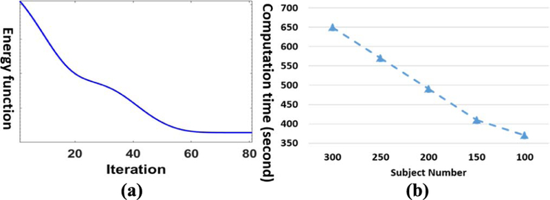
Convergence analysis and computational time w.r.t. subject number. (a) The decrease of energy function value in optimization. (b) Computation time vs subject number.

D. Evaluation of Classification Accuracy

Fig. 4. shows the classification performance in terms of ACC, SPEC, and SEN by ensemble SVM (blue), statistic hyper-graph (red), dynamic simple-graph (gray), and dynamic hyper-graph (yellow), in MCI/NC classification (a), MCI-C/ MCI-NC classification (b), NC/MCI/AD classification (c), and NC/MCI-C/MCI-NC/AD classification (d). It is apparent that our method outperforms all other competing methods, where the largest improvement is 8.9% increase of ACC over ensemble SVM in MCI/NC classification task. We further perform the t-test on the ACC value. Our method achieves statistically significant improvement in terms of accuracy compared to those methods (p < 0.05).

Fig. 4.

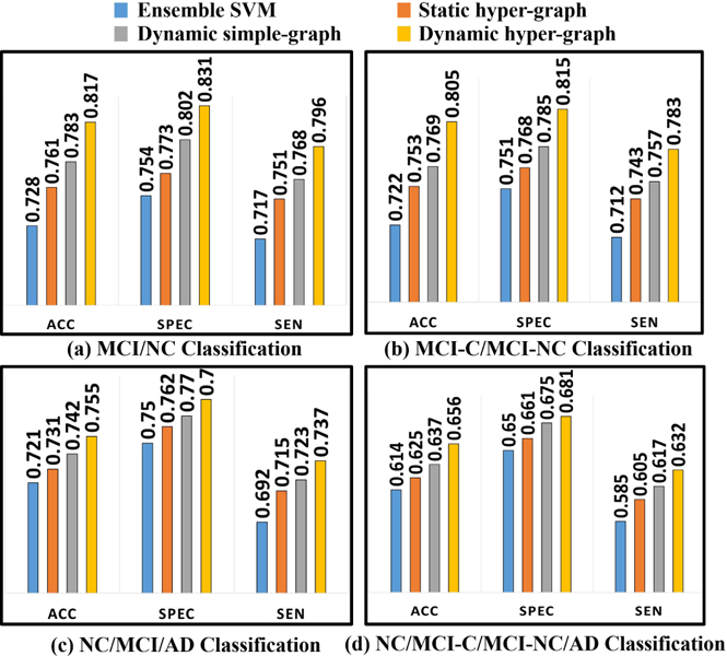
Evaluation of classification performance in terms of ACC, SEN, and SPEC by ensemble SVM (a), static hyper-graph learning (b), dynamic simple-graph learning (c), and dynamic hyper-graph learning (d).

Unlike the supervised learning approaches like SVM, our hyper-graph model needs to update to reflect the new data representation for new testing subjects. Also, the classification performance could vary with different ratio of training and testing subjects in the hyper-graph. Here, we specifically inspect the ACC value w.r.t. the ratio of training and testing subjects in NC/MCI/AD classification (Fig. 5(a)) and NC/MCI-C/MCI-NC/AD classification (Fig. 5(b)), where blue, red, gray, and yellow curves represent ensemble SVM, static hyper-graph, dynamic simple graph, and dynamic hyper-graph methods, respectively. Note, we fix the total number of subjects while changing the ratio. It is consistent that the more training subjects (with clinical labels) included in the hyper-graph, the higher classification accuracy the learned model can achieve.

Fig. 5.

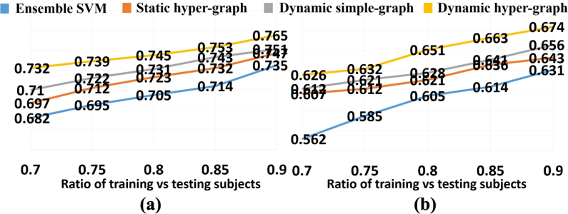
ACC curve w.r.t. the ratio of training vs testing subjects in NC/MCI/AD classification (a) and NC/MCI-C/MCI-NC/AD classifica-tion (b).

In order to evaluate whether the classification performance of our method is dominated by specific group (AD or NC), we show the accuracy, sensitivity and specificity by class label in Table I. The best performance is on AD group (ACC 0.671, SEN 0. 706 and SPEC 0.655) and the worst performance is on MCI-NC group (ACC 0.633, SEN 0.656 and SPEC 0.623). The performance difference between different groups is smaller than 0.4%. This indicates that the performance of our method is not dominated by AD or NC subjects. It is balanced well on all groups, especially on the MCI-C and MCI-NC groups.

TABLE I.

The Classification (MCI-C/MCI-NC/AD/NC) Results OF Dynamic Hyper-Graph Measured by Class Label (ACC-Accuracy, Sen-Sensitivity, Spec-Specificity)

	ACC	SPEC	SEN
MCI-C	0.633	0.656	0.623
MCI-NC	0.628	0.653	0.621
NC	0.646	0.682	0.640
AD	0.671	0.706	0.655

E. Evaluation of Regression Accuracy

Similarly, we first show the regression accuracy of ADAD-COG and MMSE score based on CC in Fig. 6(a) and RMSE in Fig. 6(b), where we use the same legend for the methods under comparison as in Fig. 4. We also performed a t-test on the CC value, where our dynamic hyper-graph learning method achieves significant improvement over other ensemble SVR, static hyper graph, and dynamic simple graph (p-value < .0.05). The curve of CC value change in ADAS-COG and MMSE regression tasks w.r.t. the ratio of training and testing subjects are shown in Fig. 7(a) and (b), respectively. We observed the same pattern that more prior knowledge on clinical score brings higher regression accuracy.

Fig. 6.

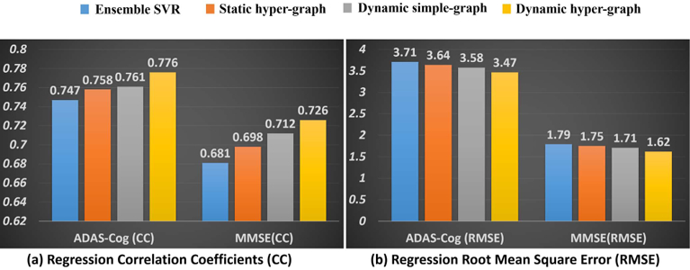
Evaluation of regression performance in terms of CC (a) and RMSE (b) by ensemble SVR (blue), static hyper-graph learning (orange), dynamic simple-graph learning (gray), and dynamic hyper-graph learning (yellow).

Fig. 7.

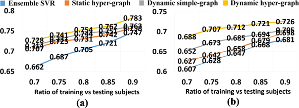
CC curve w.r.t. the ratio of training vs testing subjects in ADAS-COG score regression (a) and MMSE score regression (b).

F. Evaluation of Joint Classification and Regression

We applied our dynamic hyper-graph learning model to jointly identify the clinical labels (NC/MCI-C/MCI-NC/AD) and scores (ADAS-COG/MMSE) for all 312 subjects. Since it is not straightforward to extend the SVM approach to the joint classification and regression scenario, we only compare the static hyper-graph and dynamic simple-graph methods, as shown in Fig. 8. Since we have shown the classification only and regression only results in Fig. 4 and Fig. 6, we further dis-play the gain from joint classification and regression with red and blue arrows in Fig. 8, respectively. It is apparent that the diagnostic label and score are complementary information and integrating both can substantially improve the classification and regression accuracy. We performed a t-test on the ACC and CC value; the p-value of our method compared to static hyper-graph and dynamic simple graph are 0.033 and 0.042 by ACC, and the p-value of our method compared to static hyper-graph and dynamic hyper-graph are 0.029 and 0.038 respectively on CC value.

Fig. 8.

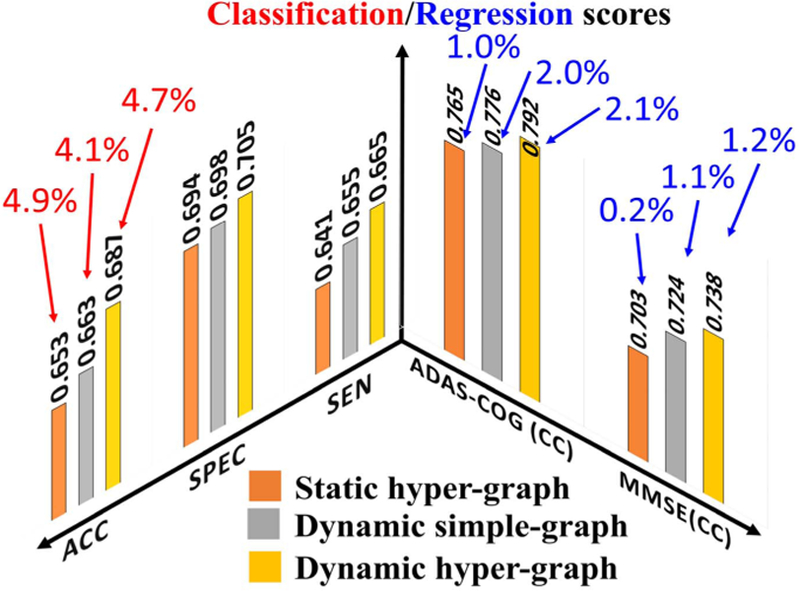
Evaluation of joint classification and regression performance by static hyper-graph learning, dynamic simple-graph learning, and dynamic hyper-graph learning methods. The improvement gained by joint classification and regression over using classification only and regression only are illustrated by red and blue arrows, respectively.

G. Enhanced Dynamic Hyper-Graph With Metric Learning

As we discussed in section III.E, we can further improve the diagnostic accuracy by integrating a metric learning technique. For clarity, we only show the classification scores of ACC, SPEC and SEN and the regression scores of CC and RMSE on ADAS-COG before and after the integration with metric leaning in Table II. Based on the scores shown in Table II, we can see the gain by using metric learning in both classification and regression.

TABLE II.

The Classification AND Regression Score Before AND After the Integration With Metric Learning

	ACC	SPEC	SEN	CC	RMSE
Before	0.687	0.705	0.665	0.792	3.34
After	0.694	0.717	0.675	0.806	3.17

H. Dynamic Hyper-Graph Learning in Missing Data Scenario

In this application, we compare the classification performance with comparison to the recent work by Liu et al. [27] where conventional static hyper-graph learning is applied to the incomplete multi-modal imaging dataset. Specifically, we randomly discard 5% to 25% imaging data while maintaining data from at least one imaging modality for each subject. Fig. 9 shows the ACC value in MCI/NC classification (a), MCI-NC/MCI-C classification (b), NC/MCI/AD classification (c), and NC/MCI-NC/MCI-C/AD classification (d), respectively. Our method consistently outperforms the conventional hyper-graph method with, on average, more than 9% improvement of classification accuracy in all classification tasks. As the percentile of missing data increases, the performance gain over the conventional method increases too, demonstrating the advantage of our dynamic hyper-graph learning method in handing incomplete imaging datasets. In order to show the statistical significance of our method compared to conventional static hyper-graph, we performed t-test on the ACC. The p-value is 0.012, which indicates that our method achieves significant improvement compared to conventional hyper-graph method in missing data scenario.

Fig. 9.

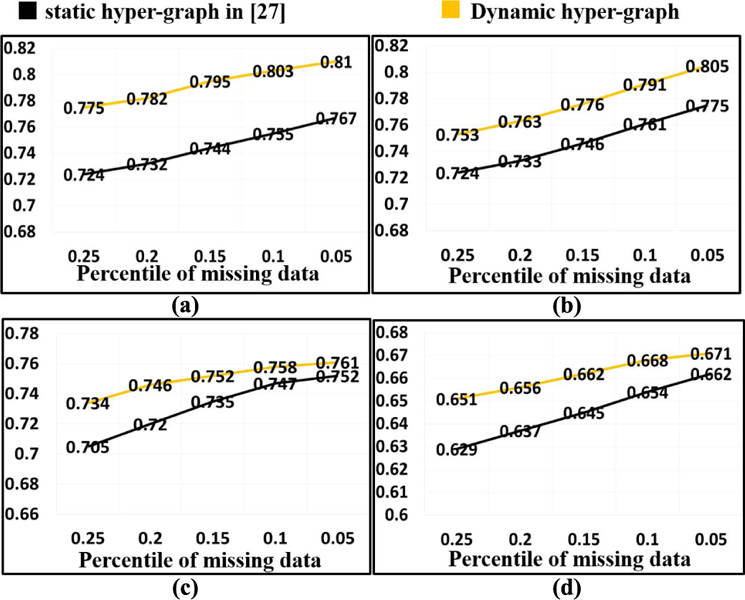
Evaluation of classification performance in missing data application by conventional hyper-graph method and our dynamic hyper-graph learning methods. (a) MCI/NC. (b) MCI-NC/MCI-C. (c) NC/MCI/AD. (d) NC/MCI-NC/MCI-C/AD.

With LOO Setting

In order to extrapolate the performance of our method to clinical settings, we compare our method with generalized and personalized SVM/SVR model for clinical label/score prediction with Leave-One-Out (LOO) testing strategy. We show that the learned personalized SVM and SVR performs comparably to our dynamic hyper-graph methods in Table III. In fact, the dynamic hyper-graph performs slightly better since it is a semi-supervised model that uses both the testing and training data to refine the model. LOO will slightly alter the performance of our method since .the labels of the testing data might change when different testing subjects are used. Overall, our model shows better performance than -supervised methods since our method uses the entire dataset to learn the hyper-graph and predict testing data labels. A t-test on the ACC value of our method compared to the generalized and personalized models yielded the following: our method vs. the generalized classifier (p = 0.037) and vs. the personalized classifier (p = 0.046); our method vs. the generalized and personalized regressor (p = 0.032 and p = 0.041 respectively). These results indicate that our method shows statistically significant improvement compared to both the generalized and personalized models.

TABLE III.

The Classification (NC/MCI/AD 3 Class Classification Problem) and Regression for ADAS-COG Prediction of the Proposed Dynamic Hyper-Graph With Generalized SVM/SVR and Personalized SVM/SVR

	ACC	SPEC	SEN	CC	RMSE
Dynamic HG	0.759	0.782	0.748	0.779	3.42
Generalized	0.726	0.749	0.713	0.734	3.84
Personalized	0.744	0.768	0.725	0.758	3.58

IV. CONCLUSION

We propose a dynamic hyper-graph learning framework for computer-assisted diagnosis using multi-modal imaging data. Specifically, we present a unified learning approach to jointly estimating the data representation using hyper-graph and performed classification and regression on the learned hyper-graph representation. Our novel approach yielded promising results in identifying the diagnostic labels and predicting clinical scores in subjects who lie along the MCI – AD clinical spectrum. In the future, we will investigate the potential application of our proposed dynamic hyper-graph learning method to other neurodegenerative diseases such as Parkinson’s disease and related Lewy body disorders.

REFERENCES

- [1].Braak H and Braak E, “Neuropathological stageing of Alzheimer-related changes,” Acta Neuropathol, vol. 82, no. 4, pp. 239–259, 1991. [DOI] [PubMed] [Google Scholar]
- [2].Liu S et al. , “Multimodal neuroimaging feature learning for multiclass diagnosis of Alzheimer’s disease,” IEEE Trans. Biomed. Eng, vol. 62, no. 4, pp. 1132–1141, April 2015. [DOI] [PMC free article] [PubMed] [Google Scholar]
- [3].Mattsson N et al. , “CSF biomarkers and incipient Alzheimer disease in patients with mild cognitive impairment,” JAMA, vol. 302, no. 4, pp. 385–893, 2009. [DOI] [PubMed] [Google Scholar]
- [4].Thompson PM et al. , “Tracking Alzheimer’s disease,” Ann. New York Acad. Sci. USA, vol. 1097, no. 1, pp. 183–214, 2007. [DOI] [PMC free article] [PubMed] [Google Scholar]
- [5].Thompson PM, Hayashi KM, De Zubicaray G, Janke AL, Rose SE, and Semple J, “Dynamics of gray matter loss in Alzheimer’s disease,” J. Neurosci, vol. 23, no. 3, pp. 994–1005, 2003. [DOI] [PMC free article] [PubMed] [Google Scholar]
- [6].Wang Z et al. , “Multi-modal classification of neurodegenerative disease by progressive graph-based transductive learning,” Med. Image Anal, vol. 39, pp. 218–230, July 2017. [DOI] [PMC free article] [PubMed] [Google Scholar]
- [7].Gray K, Aljabar P, Heckemann RA, Hammers A, and Rueckert D, “Random forest-based similarity measures for multi-modal classification of Alzheimer’s disease,” NeuroImage, vol. 65, pp. 75–167, January 2013. [DOI] [PMC free article] [PubMed] [Google Scholar]
- [8].Tong T, Gray K, Gao Q, Chen L, and Rueckert D, “Nonlinear graph fusion for multi-modal classification of Alzheimer’s disease,” presented at the MICCAI, Munich, Germany, 2015. [Google Scholar]
- [9].Gao Y et al. , “MCI identification by joint learning on multiple MRI data,” presented at the MICCAI Germany, 2015. [DOI] [PMC free article] [PubMed] [Google Scholar]
- [10].Zhang D and Shen D, “Multi-modal multi-task learning for joint pre-diction of multiple regression and classification variables in Alzheimer’s disease,” NeuroImage, vol. 59, no. 2, pp. 895–907, 2012. [DOI] [PMC free article] [PubMed] [Google Scholar]
- [11].Suk HI, Lee S-W, and Shen D, “Hierarchical feature representation and multimodal fusion with deep learning for AD/MCI diagnosis,” NeuroImage, vol. 101, pp. 569–582, November 2014. [DOI] [PMC free article] [PubMed] [Google Scholar]
- [12].Wang B, Tu Z, and Tsotsos J, “Dynamic label propagation for semi-supervised multi-class multi-label classification,” presented at the IEEE Int. Conf. Comput. Vis, Portland, OR, USA, 2013. [Google Scholar]
- [13].Zhang D, Wang Y, Zhou L, Yuan H, and Shen D, “Multimodal classification of Alzheimer’s disease and mild cognitive impairment,” NeuroImage, vol. 55, pp. 856–867, April 2011. [DOI] [PMC free article] [PubMed] [Google Scholar]
- [14].Filipovych R and Davatzikos C, “Semi-supervised pattern classification of medical images: Application to mild cognitive impairment (MCI),” NeuroImage, vol. 55, pp. 1109–1119, April 2011. [DOI] [PMC free article] [PubMed] [Google Scholar]
- [15].Zhou D, Huang J, and Schölkopf B, “Learning with hypergraphs: Clustering, classification, and embedding,” presented at the Adv. Neural Inf. Process. Syst, 2006. [Google Scholar]
- [16].Dong P, Guo Y, Shen D, and Wu G, “Multi-atlas and multi-modal hippocampus segmentation for infant MR brain images by propagating anatomical labels on hypergraph,” presented at the 1st Int. Workshop Patch-Based Techn. Med. Imag, Munich, Germany, 2015. [DOI] [PMC free article] [PubMed] [Google Scholar]
- [17].Liu M, Zhang J, Yap P-T, and Shen D, “Diagnosis of Alzheimer’s disease using view-aligned hypergraph learning with incomplete multi-modality data,” presented at the MICCAI, Athens, Greece, 2016. [DOI] [PMC free article] [PubMed] [Google Scholar]
- [18].Wang H, Nie F, Huang H, Risacher S, Saykin AJ, and Shen L, “Identifying AD-sensitive and cognition-relevant imaging biomarkers via joint classification and regression,” presented at the Med. Image Comput. Comput. Assist. Intervent, 2011. [DOI] [PMC free article] [PubMed] [Google Scholar]
- [19].Boyd S and Vandenberghe L, Convex Optimization Cambridge, U.K.: Cambridge Univ. Press, 2009. [Google Scholar]
- [20].Rosen WG, Mohs RC, and Davis KL, “A new rating scale for Alzheimer’s disease,” Amer. J. Psychiatry, vol. 141, pp. 1356–1364, November 1984. [DOI] [PubMed] [Google Scholar]
- [21].Tombaugh TN and McIntyre NJ, “The mini-mental state examination: A comprehensive review,” J. Amer. Geriatrics Soc, vol. 40, no. 9, pp. 922–935, 1992. [DOI] [PubMed] [Google Scholar]
- [22].Nie F, Wang X, and Huang H, “Clustering and projected clustering with adaptive neighbors,” presented at the 20th ACM SIGKDD Conf. Knowl. Discovery Data Mining (KDD), New York, NY, USA, 2014. [Google Scholar]
- [23].Kulis B, “Metric learning: A survey,” Found. Trends Mach. Learn, vol. 5, no. 4, pp. 287–364, 2013. [Google Scholar]
- [24].Shi B, Wang Z, and Liu J, “Distance-informed metric learning for Alzheimer’s disease staging,” presented at the 36th Annu. Int. Conf. IEEE Eng. Med. Biol. Soc. (EMBC), Chicago, IL, USA, 2014. [DOI] [PubMed] [Google Scholar]
- [25].Coley N et al. , “How should we deal with missing data in clinical trials involving Alzheimer’s disease patients?” Current Alzheimer Res, vol. 8, no. 4, pp. 421–433, 2011. [DOI] [PubMed] [Google Scholar]
- [26].Belger M et al. , “How to deal with missing longitudinal data in cost of illness analysis in Alzheimer’s disease-suggestions from the GERAS observational study,” BMC Med. Res. Methodol, vol. 16, no. 1, p. 83, 2016. [DOI] [PMC free article] [PubMed] [Google Scholar]
- [27].Liu M, Zhang J, Yap P-T, and Shen D, “View-aligned hypergraph learning for Alzheimer’s disease diagnosis with incomplete multi-modality data,” Med. Image Anal, vol. 36, pp. 123–134, February 2017. [DOI] [PMC free article] [PubMed] [Google Scholar]
- [28].Nestor PJ, Scheltens P, and Hodges JR, “Advances in the early detection of Alzheimer’s disease,” Nature Rev. Neurosci, vol. 5, pp. S34–S41, July 2004. [DOI] [PubMed] [Google Scholar]
- [29].Morrison JH and Hof PR, “Life and death of neurons in the aging brain,” Science, vol. 278, pp. 412–419, October 1997. [DOI] [PubMed] [Google Scholar]
- [30].Cuingnet R et al. , “Automatic classification of patients with Alzheimer’s disease from structural MRI: A comparison of ten methods using the ADNI database,” NeuroImage, vol. 56, no. 2, pp. 766–781, 2011. [DOI] [PubMed] [Google Scholar]
- [31].Driscoll I et al. , “ Longitudinal pattern of regional brain volume change differentiates normal aging from MCI,” Neurology, vol. 72, no. 22, pp. 1906–1913, 2009. [DOI] [PMC free article] [PubMed] [Google Scholar]
- [32].Reisberg B, Ferris SH, Kluger A, Franssen E, Wegiel J, and de Leon MJ, “Mild cognitive impairment (MCI): A historical perspective,” Int. Psychogeriatrics, vol. 20, no. 1, pp. 18–31, 2008. [DOI] [PubMed] [Google Scholar]
- [33].Shi F, Wang L, Dai Y, Gilmore JH, Lin W, and Shen D, “LABEL: Pediatric Brain Extraction using Learning-based Meta-algorithm,” Neu-roImage, vol. 62, no. 3, pp. 1975–1986, 2012. [DOI] [PMC free article] [PubMed] [Google Scholar]
- [34].Tustison NJ et al. , “N4ITK: Improved N3 bias correction,” IEEE Trans. Med. Imag, vol. 29, no. 6, pp. 1310–1320, June 2010. [DOI] [PMC free article] [PubMed] [Google Scholar]
- [35].Madabhushi A and Udupa JK, “New methods of MR image intensity standardization via generalized scale,” Med. Phys, vol. 33, no. 9, pp. 3426–3434, 2006. [DOI] [PubMed] [Google Scholar]
- [36].Varoquaux G, Raamana PR, Engemann DA, Hoyos-Idrobo A, Schwartz Y, and Thirion B, “Assessing and tuning brain decoders: Cross-validation, caveats, and guidelines,” NeuroImage, vol. 145, pp. 166–179, January 2017. [DOI] [PubMed] [Google Scholar]
- [37].Zhu Y, Kim M, Zhu X, Yan J, Kaufer D, and Wu G, “Personalized diagnosis for Alzheimer’s disease,” in Proc. MICCAI, 2017, pp. 205–213. [DOI] [PMC free article] [PubMed] [Google Scholar]