Minimum sample size for developing a multivariable prediction model: PART II ‐ binary and time‐to‐event outcomes

Abstract

When designing a study to develop a new prediction model with binary or time‐to‐event outcomes, researchers should ensure their sample size is adequate in terms of the number of participants (n) and outcome events (E) relative to the number of predictor parameters (p) considered for inclusion. We propose that the minimum values of n and E (and subsequently the minimum number of events per predictor parameter, EPP) should be calculated to meet the following three criteria: (i) small optimism in predictor effect estimates as defined by a global shrinkage factor of ≥0.9, (ii) small absolute difference of ≤ 0.05 in the model's apparent and adjusted Nagelkerke's R², and (iii) precise estimation of the overall risk in the population. Criteria (i) and (ii) aim to reduce overfitting conditional on a chosen p, and require prespecification of the model's anticipated Cox‐Snell R², which we show can be obtained from previous studies. The values of n and E that meet all three criteria provides the minimum sample size required for model development. Upon application of our approach, a new diagnostic model for Chagas disease requires an EPP of at least 4.8 and a new prognostic model for recurrent venous thromboembolism requires an EPP of at least 23. This reinforces why rules of thumb (eg, 10 EPP) should be avoided. Researchers might additionally ensure the sample size gives precise estimates of key predictor effects; this is especially important when key categorical predictors have few events in some categories, as this may substantially increase the numbers required.

1. INTRODUCTION

Statistical models for risk prediction are needed to inform clinical diagnosis and prognosis in healthcare.1, 2, 3 For example, they may be used to predict an individual's risk of having an undiagnosed disease or condition (“diagnostic prediction model”), or to predict an individual's risk of experiencing a specific event in the future (“prognostic prediction model”). They are typically developed using a multivariable regression framework, such as logistic or Cox (proportional hazards) regression, which provides an equation to estimate an individual's risk based on their values of multiple predictors (such as age and smoking, or biomarkers and genetic information). Well‐known examples are the Wells score for predicting the presence of a pulmonary embolism4, 5; the Framingham risk score and QRISK2,6, 7 which estimate the 10‐year risk of developing cardiovascular disease (CVD); and the Nottingham Prognostic Index, which predicts the 5‐year survival probability of a woman with newly diagnosed breast cancer.8, 9

Researchers planning or designing a study to develop a new multivariable prediction model must consider sample size requirements for their development data set. Our related paper considered this issue for prediction models of a continuous outcome using linear regression.10 Here, we focus on binary and time‐to‐event outcomes, such as the risk of already having a pulmonary embolism, or the risk of developing CVD in the next 10 years. In this situation, the effective sample size is often considered to be the number of outcome events (eg, the number with existing pulmonary embolism, or the number diagnosed with CVD during follow‐up). In particular, a well‐used “rule of thumb” for sample size is to ensure at least 10 events per candidate predictor (variable),11, 12, 13 where “candidate” indicates a predictor in the development data set that is considered, before any variable selection, for inclusion in the final model. Note that, if a predictor is categorical with three of more categories, or continuous and modelled as a nonlinear trend, then including the predictor will require two or more parameters being included in the model. Therefore, we refer to events per predictor parameter (EPP) here, rather than events per variable.

The 10 EPP rule has generated much debate. Some authors claim that the EPP can sometimes be lowered below 10.14 In contrast, Harrell generally recommends at least 15 EPP,15 and others identify situations where at least 20 EPP or up to 50 EPP are required.16, 17, 18, 19 However, a concern is that any blanket rule of thumb is too simplistic, and that the number of participants required will depend on many intricate aspects, including the magnitude of predictor effects, the overall outcome risk, the distribution of predictors, and the number of events for each category of categorical predictors.16 For example, Courvoisier et al20 concluded that “There is no single rule based on EPP that would guarantee an accurate estimation of logistic regression parameters.” A new sample size approach is needed to address this.

In this article, we propose the sample size (n) and number of events (E) in the model development data set must, at the very least, meet the following three criteria: (i) small optimism in predictor effect estimates as defined by a global shrinkage factor of ≥0.9, (ii) small absolute difference of ≤ 0.05 in the model's apparent and adjusted Nagelkerke's R², and (iii) precise estimation of the overall risk or rate in the population (or similarly, precise estimation of the model intercept when predictors are mean centred). The values of n and E (and subsequently EPP) that meet all three criteria provide the minimum values required for model development. Criteria (i) and (ii) aim to reduce the potential for a developed model to be overfitted to the development data set at hand. Overfitting leads to model predictions that are more extreme than they ought to be when applied to new individuals, and most notably occurs when the number of candidate predictors is large relative to the number of outcome events. A consequence is that a developed model's apparent predictive performance (as observed in the development data set itself) will be optimistic, and its performance in new data will usually be lower. Therefore, it is good practise to reduce the potential for overfitting when developing a prediction model,15 which criteria (i) and (ii) aim to achieve. In addition, criterion (iii) aims to ensure that the overall risk (eg, by a key time point for prediction) is estimated precisely, as fundamentally, before tailoring predictions to individuals, a model must be able to reliably predict the overall or mean risk in the target population.

The article is structured as follows. Section 2 introduces our proposed criterion (i), for which key concepts of a global shrinkage factor and the Cox‐Snell R² are introduced.21 The latter needs to prespecified to utilise our sample size formula, and so in Section 3, we suggest how realistic values of the Cox‐Snell R² can be obtained in advance of any data collection, eg, by using published information from an existing model in the same field, including values of the C statistic or alternative R² measures. Extension to criteria (ii) and (iii) is then made in Section 4. Section 5 then provides two examples, which demonstrate our sample size approach for diagnostic and prognostic models. Section 6 raises a potential additional criteria to consider: ensuring precise estimates of key predictor effects, to help ensure precise predictions across the entire spectrum of predicted risk. Section 7 concludes with discussion.

2. SAMPLE SIZE REQUIRED TO MINIMISE OVERFITTING OF PREDICTOR EFFECTS

To adjust for overfitting during model development (and thereby improve the model's predictive performance in new individuals), statistical methods for penalisation of predictor effect estimates are available, where regression coefficients are shrunk toward zero from their usual estimated value (eg, from standard maximum likelihood estimation).22, 23, 24, 25, 26 Van Houwelingen notes that “… shrinkage works on the average but may fail in the particular unique problem on which the statistician is working.” 22 Therefore, it is important to minimise the potential for overfitting during model development, and this criterion forms the basis of our first sample size calculation. Our approach is motivated by the concept of a global shrinkage factor (a measure of overfitting), and so we begin by introducing this, before then deriving a sample size formula.

2.1. Concept of a global shrinkage for logistic and Cox regression

The concept of shrinkage (penalisation) was outlined in our accompanying paper,10 and is explained in detail elsewhere.1, 15, 27 Here, we focus on using a global shrinkage factor (S), sometimes referred to as a uniform shrinkage factor. Consider a logistic regression model has been fitted using standard maximum likelihood estimation (ie, traditional and unpenalised estimation). Subsequently, S can be estimated (eg, using bootstrapping,28 or via a closed‐form solution; see Section 2.2) and applied to the estimated predictor effects, so that the revised model is

$$\ln \left(\frac{p_i}{1-p_i}\right)={\alpha }^{*}+S\left({\widehat{\beta }}_1{X}_{1i}+{\widehat{\beta }}_2{X}_{2i}+{\widehat{\beta }}_3{X}_{3i}+\text{⋯}\right).$$ (1)

Here, p_i is the outcome probability for the ith individual, the $\widehat{\beta }$ terms denote the original predictor effect estimates (ln odds ratios) from maximum likelihood, and α^* is the intercept that has been re‐estimated (after shrinkage of predictor effects) to ensure perfect calibration‐in‐the‐large, such that, the overall predicted risk still agrees with the overall observed risk in the development data set (for details on how to do this, we refer to the works of Harrell15 and Steyerberg1). Similarly, after fitting a proportional hazards (Cox) regression model using standard maximum likelihood, the model can be revised using

$$h_i\left(t\right)=h_0{\left(t\right)}^{*}\exp \left(S\left({\widehat{\beta }}_1{X}_{1i}+{\widehat{\beta }}_2{X}_{2i}+{\widehat{\beta }}_3{X}_{3i}+\text{⋯}\right)\right),$$ (2)

where h_i(t) is the hazard rate of the outcome over time (t) for the ith individual and h_o(t)^* is the baseline hazard function re‐estimated (after shrinkage of predictor effects) to ensure the predicted and observed outcome rates agree for the development data set as whole. Compared to the original (nonpenalised) models, the revised models (1) and (2) will shrink predicted probabilities away from zero and one, toward the overall mean outcome probability in the development data set.

Example of a global shrinkage factor

Van Diepen et al developed a prognostic model for 1‐year mortality risk in patients with diabetes starting dialysis.29 They use a logistic regression framework, with backwards selection to choose predictors in a dataset of 394 patients with 84 deaths by 1 year, and the estimated model is shown in Table 1. To examine overfitting, the authors use bootstrapping to estimate a global shrinkage factor of 0.903, indicating that the original model was slightly overfitted to the data. Therefore, a revised prediction model was produced by multiplying the original $\widehat{\beta }$ coefficients (ln odds ratios) from the original logistic regression model by a global shrinkage factor of S = 0.903.

Table 1.

Example of global shrinkage applied to a prognostic model for 1‐year mortality risk in patients with diabetes starting dialysis29

	Developed (unpenalised) model	Final (penalised) model adjusted for overfitting
Intercept	$\widehat{\mathit{\alpha }}$	α*
	1.962	1.427
Predictor	$\widehat{\mathit{\beta }}$	$\mathit{S}\widehat{\mathit{\beta }}$ = 0.903 $\widehat{\mathit{\beta }}$
Age (years)	0.047	0.042
Smoking	0.631	0.570
Macrovascular complications	1.195	1.078
Duration of diabetes mellitus (years)	0.026	0.023
Karnofsky scale	−0.043	−0.039
Haemoglobin level (g/dl)	−0.186	−0.168
Albumin level (g/l)	−0.060	−0.054

2.2. Expressing sample size in terms of a global shrinkage factor

Bootstrapping is an excellent way to calculate the shrinkage factor postestimation, but (as it is a resampling method) is not useful for us in advance of data collection. An alternative approach to calculating a global shrinkage factor is to use the closed form “heuristic” shrinkage factor of Van Houwelingen and Le Cessie,23 defined by

$$S_{VH}=1-\frac{p}{\mathrm{LR}},$$ (3)

where p is the total number of predictor parameters for the full set of candidate predictors (ie, all those considered for inclusion in the model) and LR is the likelihood ratio (chi‐squared) statistic for the fitted model defined as

$$\mathrm{LR}=-2\left(\ln L_{\mathrm{\text{null}}}-\ln L_{\mathrm{\text{model}}}\right),$$ (4)

where ln L_null is the log‐likelihood of a model with no predictors (eg, intercept‐only logistic regression model), and ln L_model is the log‐likelihood of the final model. In our related paper on linear regression, we used the Copas shrinkage estimate that is similar to Equation (3), but with p replaced by p + 2. In our experience, S_VH performs better for generalised linear models than the Copas estimate, with S_VH further from 1 and closer to the corresponding estimate obtained from bootstrapping. Copas also notes that, unlike for linear regression, a formal justification for replacing p by p + 2 in Equation (2) has not been proved for logistic regression.30

Hence, we use Equation (3) as our shrinkage estimate (ie, our measure of overfitting) for logistic and Cox regression models, which now motivates our sample size approach to meet criterion (i). First, let us re‐express the right‐hand side of Equation (3) in terms of sample size (n), number of candidate predictor parameters (p), and the Cox‐Snell generalised R².21 The latter is also known as the maximum likelihood R², the likelihood ratio R², or Magee's R²,31 and it provides a generalisation (eg, to logistic and Cox regression models) of the well‐known proportion of variance explained for linear regression models. Let us use $R_{\mathrm{CS}\text{\_}\mathrm{app}}^2$ to denote the apparent (“app”) estimate of a prediction model's Cox‐Snell (“CS”) R² performance as obtained from the model development data set. It can be shown (eg, see the works of Magee31 or Hendry and Nielsen32) that the LR statistic can be expressed in terms of the sample size (n) and $R_{\mathrm{CS}\text{\_}\mathrm{app}}^2$ as follows:

$$\mathrm{LR}=-n\ln \left(1-R_{\mathrm{CS}\text{\_}\mathrm{app}}^2\right).$$ (5)

This leads to the Cox‐Snell generalised definition of the apparent R² expressed in terms of the LR value for any regression model, including logistic and Cox regression

$$R_{\mathrm{CS}\text{\_}\mathrm{app}}^2=1-\exp \left(\frac{-\mathrm{LR}}{n}\right).$$ (6)

Applying Equation (5) within Equation (3), the Van Houwelingen and Le Cessie shrinkage factor becomes

$$S_{VH}=1+\frac{p}{n\ln \left(1-R_{\mathrm{CS}\text{\_}\mathrm{app}}^2\right)}.$$ (7)

2.3. Criterion (i): calculating sample size to ensure a shrinkage factor ≥ 0.9

Equation (7) provides a closed‐form solution for the expected shrinkage conditional on n, p, and $R_{\mathrm{CS}\text{\_}\mathrm{app}}^2$. Therefore, if we could specify a realistic value for $R_{\mathrm{CS}\text{\_}\mathrm{app}}^2$ in advance of our study starting, we could identify values of n and p that correspond to a desired shrinkage factor (eg, 0.9), thus informing the required sample size. However, a major problem is that $R_{\mathrm{CS}\text{\_}\mathrm{app}}^2$ is a postestimation measure of model fit, whereas for a sample size calculation, this needs to be specified in advance of collecting the data when designing a new study. Furthermore, due to overfitting in the model development data set, the observed $R_{\mathrm{CS}\text{\_}\mathrm{app}}^2$ is generally an upwardly biased (optimistic) estimate of the Cox‐Snell R² as it is estimated in the same data used to develop the model. Thus, in new data, the actual Cox‐Snell R² peformance is likely to be lower.

Therefore, we need to re‐express S_VH in terms of $R_{\mathrm{CS}\text{\_}\mathrm{adj}}^2$, an adjusted (approximately unbiased) estimate of the model's expected $R_{\mathrm{CS}}^2$performance in new individuals from the same population. In other words, $R_{\mathrm{CS}\text{\_}\mathrm{adj}}^2$ is a modification of $R_{\mathrm{CS}\text{\_}\mathrm{app}}^2$ to adjust for optimism (caused by overfitting) in the model development data set. For generalised linear models such as logistic regression, Mittlboeck and Heinzl suggest that $R_{\mathrm{CS}\text{\_}\mathrm{adj}}^2$ can be obtained by33

$$R_{\mathrm{CS}\text{\_}\mathrm{adj}}^2=S_{VH}{R}_{\mathrm{CS}\text{\_}\mathrm{app}}^2$$ (8)

as the expected value of this $R_{\mathrm{CS}\text{\_}\mathrm{adj}}^2$ corresponds to the underlying population value.33 By rearranging Equation (8), we can express $R_{\mathrm{CS}\text{\_}\mathrm{app}}^2$ in terms of $R_{\mathrm{CS}\text{\_}\mathrm{adj}}^2$

$$R_{\mathrm{CS}\text{\_}\mathrm{app}}^2=\frac{R_{\mathrm{CS}\text{\_}\mathrm{adj}}^2}{S_{VH}}.$$ (9)

Applying Equation (9) within Equation (7), we can now express S_VH in terms of $R_{\mathrm{CS}\text{\_}\mathrm{adj}}^2$, rather than $R_{\mathrm{CS}\text{\_}\mathrm{app}}^2$

$$S_{VH}=1+\frac{p}{n\ln \left(1-\frac{R_{\mathrm{CS}\text{\_}\mathrm{adj}}^2}{S_{VH}}\right)}.$$ (10)

Finally, a simple rearrangement of Equation (10) leads to a closed‐form solution for the required sample size to develop a prediction model conditional on p, S_VH and $R_{\mathrm{CS}\text{\_}\mathrm{adj}}^2$

$$n=\frac{p}{\left(S_{VH}-1\right)\ln \left(1-\frac{R_{\mathrm{CS}\text{\_}\mathrm{adj}}^2}{S_{VH}}\right)}.$$ (11)

For example, for developing a new logistic regression model based on up to 20 candidate predictor parameters with an anticipated $R_{\mathrm{CS}\text{\_}\mathrm{adj}}^2$ of at least 0.1, then to target an expected shrinkage of 0.9, we need a sample size of

$$n=\frac{p}{\left(S_{VH}-1\right)\ln \left(1-\frac{R_{\mathrm{CS}\text{\_}\mathrm{adj}}^2}{S_{VH}}\right)}=\frac{20}{\left(0.9-1\right)\ln \left(1-\frac{0.1}{0.9}\right)}=1698,$$

and thus 1698 individuals.

2.4. Translating the calculated sample size to the number of events and EPP

It may be surprising that the overall outcome proportion (or overall outcome rate) is not directly included in the right‐hand side of the sample size Equation (11), especially because the total number of events, E, (which depends on the outcome proportion or rate) is often considered the effective sample size for binary and time‐to‐event outcomes.15 However, the outcome proportion (rate) is indirectly accounted for in the sample size calculation via the chosen $R_{\mathrm{CS}\text{\_}\mathrm{adj}}^2$, as the maximum value of $R_{\mathrm{CS}\text{\_}\mathrm{adj}}^2$ for the intended population of the model depends on the overall outcome proportion (rate) for that population. As the outcome proportion decreases, the maximum value of $R_{\mathrm{CS}}^2$ decreases. This is explained further in Section 3.4. Therefore, after n is derived from the sample size equation (11), E can be obtained by combining the calculated n with the outcome proportion (rate) for the intended population. Similarly, EPP can be obtained.

For example for binary outcomes, E = nϕ and EPP = nϕ/p, where ϕ is the overall outcome proportion in the target population (ie, the overall prevalence for diagnostic models, or the overall cumulative incidence by a key time point for prognostic models). In our aforementioned hypothetical example, where 1698 subjects were needed based on an $R_{\text{CS}\text{\_}\text{adj}}^2$ of 0.1 and S_VH of 0.9, then if the intended setting has ϕ of 0.1 (ie, overall outcome risk is 10%), the required E = 1698 × 0.1 = 169.8. With 20 predictor parameters, the required EPP = (1698 × 0.1)/20= 8.5. However, if the intended setting has ϕ of 0.3, then E = 509.4 and EPP = 25.5. The big change in EPP is because, although the chosen value of $R_{\mathrm{CS}\text{\_}\mathrm{adj}}^2$ is fixed at 0.1, the maximum value of $R_{\mathrm{CS}}^2$ is much higher for the setting with the higher outcome proportion.

We can explain this further using Nagelkerke's “proportion of total variance explained”,34 which is calculated as $R_{\mathrm{CS}\text{\_}\mathrm{adj}}^2/\max \left(R_{\mathrm{CS}}^2\right)$. If two models have the same $R_{\mathrm{CS}\text{\_}\mathrm{adj}}^2$ (say at 0.1, as in the aforementioned examples), then Nagelkerke's measure of predictive performance will be lower for the model whose setting has a higher outcome proportion, as the $\max \left(R_{\mathrm{CS}}^2\right)$ is larger in that setting. Models with lower performance have larger overfitting concerns,22 and therefore require larger EPP to minimise overfitting than models with high performance. Hence, explaining why EPP was larger when ϕ was 0.3 compared with 0.1 in the aforementioned example. This highlights that a blanket rule of thumb (such as at least 10 EPP) is unlikely to be sensible to meet criterion (i), as the actual EPP depends on the setting/population of interest (which dictates the overall outcome proportion or rate) and expected model performance.

3. HOW TO PRESPECIFY ${\mathit{R}}_{\mathbf{\text{CS}}\text{\_}\mathbf{\text{adj}}}^{\mathbf{2}}$ BASED ON PREVIOUS INFORMATION

Our sample size proposal in Equation (11) requires researchers to provide a value for the model's $R_{\text{CS}\text{\_}\text{adj}}^2$, that is, to prespecify the anticipated Cox‐Snell R² value if the model was applied to new individuals. How should this be done? We recommend using $R_{\text{CS}\text{\_}\text{adj}}^2$ values from previous prediction model studies for the same (or similar) population, considering the same (or similar) outcomes and time points of interest. For example, the researcher could consult systematic reviews of existing models and their performance, which are also increasingly available,35 or registries that record the prediction models available in a particular field.36

Often, a new prediction model is developed specifically to update or improve upon the performance of an existing model, by using additional predictors. Then, the existing model's $R_{\mathrm{CS}\text{\_}\mathrm{adj}}^2$ could be used as a lower bound for the new model's anticipated $R_{\mathrm{CS}\text{\_}\mathrm{adj}}^2$. In this situation, if the apparent Cox‐Snell estimate, $R_{\mathrm{CS}\text{\_}\mathrm{app}}^2$, is available in an article describing the development of the existing model, then its $R_{\mathrm{CS}\text{\_}\mathrm{adj}}^2$ can be derived using Equation (8) as long as the study's n and p can also be obtained. In addition, as in van Diepen et al's example (Table 1), a global shrinkage factor may be reported directly for an existing model development study, and if so, $R_{\mathrm{CS}\text{\_}\mathrm{adj}}^2$ can be derived from a simple rearrangement of Equation (10), again as long as the study's n and p are also available.

Note that, if $R_{\mathrm{CS}\text{\_}\mathrm{app}}^2$ is available from an external validation study of an existing model, there is no need for adjustment (ie, $R_{\mathrm{CS}\text{\_}\mathrm{app}}^2=R_{\mathrm{CS}\text{\_}\mathrm{adj}}^2)$, as the validation dataset provides a direct estimate of the model's performance in new individuals (free from overfitting concerns as there is no model development therein).

Other options to obtain $R_{\mathrm{CS}\text{\_}\mathrm{adj}}^2$ from the existing literature are now described. For guidance on choosing an $R_{\mathrm{CS}\text{\_}\mathrm{adj}}^2$ value in the absence of any prior information, please see our discussion.

3.1. Using the LR statistic to derive the Cox‐Snell ${\mathit{R}}_{\mathbf{\text{adj}}}^{\mathbf{2}}$

If the $R_{\text{CS}\text{\_}\text{app}}^2$ or $R_{\text{CS}\text{\_}\text{adj}}^2$ is not available in the publication of an existing model, the LR value may be reported, which would allow $R_{\text{CS}\text{\_}\text{app}}^2$ to be derived using Equation (6), then S_VH for the model derived using Equation (7) (assuming the model's n and p are also provided), and finally $R_{\text{CS}\text{\_}\text{adj}}^2$ using Equation (8).

Sometimes the log‐likelihood of the final model (lnL_model) is reported, but not the LR value itself. In this situation, the researcher should calculate ln L_null based on other information in the article, and then calculate LR using Equation (4), thus allowing $R_{\mathrm{CS}\text{\_}\mathrm{app}}^2$ and $R_{\mathrm{CS}\text{\_}\mathrm{adj}}^2$ to be derived using Equations (6) and (8), respectively. For example, in a logistic regression model, the logL_null value can be calculated using

$$\ln L_{\mathrm{\text{null}}}=E\ln \left(\frac{E}{n}\right)+\left(n-E\right)\ln \left(1-\frac{E}{n}\right),$$ (12)

where E is the total number of outcome events. Of course, this assumes E and n are actually available in the article. Similarly, for an exponential survival model (equivalent to a Poisson model with ln (survival time) as an offset), the ln L_null can be calculated using

$$\ln L_{\mathrm{\text{null}}}=E\ln \left(\lambda \right)+\lambda T=E\ln \left(\frac{E}{T}\right)+E$$ (13)

as long as λ (the constant hazard rate), E (the total number of events), and T (the total time at risk, eg, total person‐years) are available in the article. Note that, for survival models, packages such as SAS and Stata usually add a constant to the reported log‐likelihood to ensure it remains the same value regardless of the time scale used. For example, Stata adds the sum of the ln (survival times) for the noncensored individuals to the reported ln L_model and ln L_null, and so this constant must be either consistently used or consistently removed in each of ln L_model and ln L_null when deriving the LR value.

3.2. Using other pseudo‐R² statistics to derive ${\mathit{R}}_{\mathbf{\text{CS}}\text{\_}\mathbf{\text{adj}}}^{\mathbf{2}}$

Sometimes other pseudo‐R² statistics are reported for logistic and survival models, rather than the Cox‐Snell version specified in Equation (6). In particular, because $R_{\text{CS}\text{\_}\text{app}}^2$ has a maximum value less than 1, Nagelkerke's R² is sometimes reported,34 which divides $R_{\text{CS}\text{\_}\text{app}}^2$ by the maximum value defined by $1-\exp \left(\frac{2\ln L_{\text{null}}}{n}\right)$, as follows:

$$R_{\mathrm{\text{Nagelkerke}}\text{\_}\mathrm{app}}^2=\frac{R_{\mathrm{CS}\text{\_}\mathrm{app}}^2}{\max \left(R_{\mathrm{CS}\text{\_}\mathrm{app}}^2\right)}=\frac{R_{\mathrm{CS}\text{\_}\mathrm{app}}^2}{1-\exp \left(\frac{2\ln L_{\mathrm{\text{null}}}}{n}\right)}.$$ (14)

Recall that ln L_null is derivable from other information, eg, using Equations (12) or (13) for logistic and exponential (Poisson) models, respectively. When Nagelkerke's R², ln L_null, and n are available, the $R_{\mathrm{CS}\text{\_}\mathrm{app}}^2$ can be calculated by rearranging Equation (14) to give

$$R_{\mathrm{CS}\text{\_}\mathrm{app}}^2=R_{\mathrm{\text{Nagelkerke}}\text{\_}\mathrm{app}}^2\left(1-\exp \left(\frac{2\ln L_{\mathrm{\text{null}}}}{n}\right)\right),$$ (15)

and then $R_{\mathrm{CS}\text{\_}\mathrm{adj}}^2$ calculated via Equation (8).

Another measure sometimes reported is McFadden's R² 37

$$R_{\mathrm{\text{McFadden}}\text{\_}\mathrm{app}}^2=1-\frac{\ln L_{\mathrm{\text{model}}}}{\ln L_{\mathrm{\text{null}}}}.$$ (16)

As ln L_null is often obtainable (see previous equation), when $R_{\mathrm{\text{McFadden}}\text{\_}\mathrm{app}}^2$ is reported, we can rearrange Equation (16) to obtain ln L_model, and subsequently derive the LR statistic using Equation (4), the Cox‐Snell $R_{\mathrm{CS}\text{\_}\mathrm{app}}^2$ from Equation (6), S_VH from Equation (7) (assuming the model's n and p are also provided), and finally $R_{\mathrm{CS}\text{\_}\mathrm{adj}}^2$ via Equation (8).

For proportional hazards survival models, O'Quigley et al suggested to modify $R_{\mathrm{CS}\text{\_}\mathrm{app}}^2$ by replacing n with the number of events (E)38

$$R_{\mathrm{O}\text{'}\mathrm{\text{Quigley}}\text{\_}\mathrm{app}}^2=1-\exp \left(\frac{-\mathrm{LR}}{E}\right).$$ (17)

Therefore, if $R_{\mathrm{O}\text{'}\mathrm{\text{Quigley}}\text{\_}\mathrm{app}}^2$ and E were reported, the LR value could be found using

$$\mathrm{LR}=-E\ln \left(1-R_{\mathrm{O}\text{'}\mathrm{\text{Quigley}}\text{\_}\mathrm{app}}^2\right),$$ (18)

and subsequently, $R_{\mathrm{CS}\text{\_}\mathrm{app}}^2$ can be obtained using Equation (6), S_VH using Equation (7), and finally $R_{\mathrm{CS}\text{\_}\mathrm{adj}}^2$ using Equation (8).

Another measure increasingly being reported for survival models is Royston's measure of explained variation,39 which is given by

$$R_{\mathrm{\text{Royston}}\text{\_}\mathrm{app}}^2=\frac{R_{\mathrm{O}\text{'}\mathrm{\text{Quigley}}\text{\_}\mathrm{app}}^2}{R_{\mathrm{O}\text{'}\mathrm{\text{Quigley}}\text{\_}\mathrm{app}}^2+\left(\frac{{\pi }^2}{6}\right)\left(1-R_{\mathrm{O}\text{'}\mathrm{\text{Quigley}}\text{\_}\mathrm{app}}^2\right)}.$$ (19)

When $R_{\mathrm{\text{Royston}}\text{\_}\mathrm{app}}^2$ is reported it can be used to obtain $R_{\mathrm{O}\text{'}\mathrm{\text{Quigley}}\text{\_}\mathrm{app}}^2$ by rearranging Equation (19) as

$$R_{\mathrm{O}\text{'}\mathrm{\text{Quigley}}\text{\_}\mathrm{app}}^2=\frac{-\frac{{\pi }^2}{6}{R}_{\mathrm{\text{Royston}}\text{\_}\mathrm{app}}^2}{\left(1-\frac{{\pi }^2}{6}\right)R_{\mathrm{\text{Royston}}\text{\_}\mathrm{app}}^2-1}.$$ (20)

This subsequently allows LR , $R_{\mathrm{CS}\text{\_}\mathrm{app}}^2$, S_VH and then $R_{\mathrm{CS}\text{\_}\mathrm{adj}}^2$ to be derived as explained previously. A similar measure to $R_{\mathrm{\text{Royston}}}^2$ is Royston and Sauerbrei's $R_D^2$,40 which can be derived from their proposed D statistic (the ln(hazard ratio) comparing two groups defined by the median value of the model's risk score in the population of application)

$$R_{D\text{\_}\mathrm{app}}^2=\frac{\frac{\pi }{8}{D}^2}{\frac{{\pi }^2}{6}+\frac{\pi }{8}{D}^2}.$$ (21)

In examples shown by Royston,39 $R_{\mathrm{\text{Royston}}\text{\_}\mathrm{app}}^2$ and $R_{D\text{\_}\mathrm{app}}^2$ are reasonably similar, and thus, we tentatively suggest $R_{D\text{\_}\mathrm{app}}^2$ as a proxy for $R_{\mathrm{\text{Royston}}\text{\_}\mathrm{app}}^2$ when only $R_{D\text{\_}\mathrm{app}}^2$ (or D) is reported; though, we recognise that further research is needed on the link between $R_{D\text{\_}\mathrm{app}}^2$ and $R_{\mathrm{\text{Royston}}}^2$.

3.3. Using values of the C statistic to derive ${\mathit{R}}_{\mathbf{\text{CS}}\text{\_}\mathbf{\text{adj}}}^{\mathbf{2}}$

Jinks et al also proposed the following equation, based on empirical evidence, for predicting Royston's D (and thus subsequently $R_{D\text{\_}\text{app}}^2$) when only the C statistic is reported for a survival model41

$$D=5.50\left(C-0.5\right)+10.26{\left(C-0.5\right)}^3.$$ (22)

Table 2 provides values of D (and corresponding values of $R_{D\text{\_}\mathrm{app}}^2$from Equation (21)) predicted from Equation (22) for selected values of the C statistic, as taken from the work of Jinks et al.41 Thus, if only the C statistic is reported, we can use Equation (22) to predict Royston's D statistic and calculate $R_{D\text{\_}\mathrm{app}}^2$ (using Equation (21)) as a proxy to $R_{\mathrm{\text{Royston}}\text{\_}\mathrm{app}}^2$, and then $R_{\mathrm{O}\text{'}\mathrm{\text{Quigley}}\text{\_}\mathrm{app}}^2$, LR, $R_{\mathrm{CS}\text{\_}\mathrm{app}}^2$ and finally $R_{\mathrm{CS}\text{\_}\mathrm{adj}}^2$ computed sequentially using the equations given previously.

Table 2.

Predicted values of the D statistic and $R_D^2$ from Equation (23) for selected values of the C statistic (values taken from table 1 in the work of Jinks et al41)

C	D	${\mathit{R}}_{\mathit{D}}^{\mathbf{2}}$		C	D	${\mathit{R}}_{\mathit{D}}^{\mathbf{2}}$
0.50	0	0		0.72	1.319	0.294
0.52	0.11	0.003		0.74	1.462	0.338
0.54	0.221	0.011		0.76	1.61	0.382
0.56	0.332	0.026		0.78	1.765	0.427
0.58	0.445	0.045		0.80	1.927	0.470
0.60	0.560	0.070		0.82	2.096	0.512
0.62	0.678	0.099		0.84	2.273	0.552
0.64	0.798	0.132		0.86	2.459	0.591
0.66	0.922	0.169		0.88	2.652	0.627
0.68	1.05	0.208		0.90	2.857	0.661
0.70	1.182	0.25		0.92	3.070	0.692

Further evaluation of the performance of Jinks' formula is required, eg, using simulation and across settings with different cumulative outcome incidences. Indeed, based on figure 5 in the work of Jinks et al,41 the potential error in the predictions of D appears to increase as C increases, and is about +/− 0.25 when C is 0.8. Nevertheless, Equation (22) serves as a good starting point and works well in our applied example (see Section 5.2.1). Further research is also needed to ascertain how to predict $R_{\mathrm{CS}}^2$ from other measures, such as Somer's D statistic.

3.4. The anticipated value of ${\mathit{R}}_{\mathbf{\text{CS}}\text{\_}\mathbf{\text{adj}}}^{\mathbf{2}}$ may be small

It is important to emphasise that the Cox‐Snell, $R_{\text{CS}}^2$, values for logistic and survival models are usually much lower than for linear regression models, with values often less than 0.3. A key reason is that (unlike for linear regression) the $R_{\text{CS}\text{\_}\text{app}}^2$ has a maximum value less than 1, defined by

$$\max \left(R_{\mathrm{CS}\text{\_}\mathrm{app}}^2\right)=1-\exp \left(\frac{2\ln L_{\mathrm{\text{null}}}}{n}\right).$$ (23)

This is because ln L_null is itself bounded for binary and time‐to‐event outcomes (see Equations (12) and (13)). For example, for a logistic regression model with an outcome proportion of 50%, using Equation (12) and an arbitrary sample size of 100, we have

$$\ln L_{\mathrm{\text{null}}}=E\ln \left(\frac{E}{n}\right)+\left(n-E\right)\ln \left(1-\frac{E}{n}\right)=50\ln \left(\frac{50}{100}\right)+\left(100-50\right)\ln \left(1-\frac{50}{100}\right)=-69.315,$$

and therefore, using Equation (23),

$$\max \left(R_{\text{CS}\text{\_}\text{app}}^2\right)=1-\text{exp}\left(\frac{2\ln L_{\text{null}}}{n}\right)=1-\text{exp}\left(\frac{-69.315}{100}\right)=0.75.$$

However, for an outcome proportion of 5%, the $\max \left(R_{\text{CS}\text{\_}\text{app}}^2\right)$ is 0.33, and for an outcome proportion of 1%, the $\max \left(R_{\text{CS}\text{\_}\text{app}}^2\right)$ is 0.11. Therefore, especially in situations where the outcome proportion is low, researchers should anticipate a model with a (seemingly) low $R_{\text{CS}\text{\_}\text{app}}^2$ value, and subsequently a low $R_{\text{CS}\text{\_}\text{adj}}^2$ value.

Low values of $R_{\text{CS}\text{\_}\text{app}}^2$ or $R_{\text{CS}\text{\_}\text{adj}}^2$ do not necessarily indicate poor model performance. Consider the following three examples. First, Poppe et al used a Cox regression to develop a model (“PREDICT‐CVD”) to predict the risk of future CVD events within two years in patients with atherosclerotic CVD,42 and directly report an $R_{\text{CS}\text{\_}\text{app}}^2$ of 0.04. However, the corresponding C statistic is 0.72, which shows discriminatory magnitude typical of many prognostic models used in practice. Second, Hippisley‐Cox and Coupland use the QResearch database to produce three models (QDiabetes) that estimates the risk of future diabetes in a general population.43 In their validation of their “model A,” there were 27 311 incident cases of diabetes recorded in 1 322 435 women (3.77 cases per 1000 person‐years) during follow‐up, and the reported $R_{\mathrm{\text{Royston}}\text{\_}\text{app}}^2$ was 0.505. Using the approach described previously to convert $R_{\mathrm{\text{Royston}}}^2$ to LR, this leads to a $R_{\text{CS}\text{\_}\text{app}}^2$ of 0.02; however, the corresponding D statistic of 2.07 and C statistic of 0.89 are large. Third, in a risk prediction model for venous thromboembolism (VTE) in women during the first 6 weeks after delivery,44 $R_{\text{CS}\text{\_}\text{app}}^2$ was 0.001 due to the extremely low event risk (7.2 per 10 000 deliveries), but the model still had important discriminatory ability as the corresponding C statistic was 0.70.

4. ADDITIONAL SAMPLE SIZE CRITERIA

Criterion (i) focuses on shrinkage of predictor effects, which is a multiplicative measure of overfitting (ie, on the relative scale). Harrell suggests to also evaluate overfitting on the absolute scale and to check key model parameters are estimated precsiely.15 We now address this with two further criteria.

4.1. Criterion (ii): ensuring a small absolute difference in the apparent and adjusted ${\mathit{R}}_{\mathbf{\text{Nagelkerke}}}^{\mathbf{2}}$

Our second criterion for minimum sample size is to ensure a small absolute difference (δ) between the model's apparent and adjusted proportion of variance explained. We suggest using Nagelkerke's R² for this purpose as, unlike the Cox‐Snell R² value, it can range between 0 and 1, and so a small difference (say ≤ 0.05) can be ubiquitously defined. Based on Equation (14), the difference in the apparent and adjusted Nagelkerke's R² can be defined as

$$\begin{array}{cc}{R}_{\mathrm{\text{Nagelkerke}}\text{\_}\mathrm{app}}^2-R_{\mathrm{\text{Nagelkerke}}\text{\_}\mathrm{adj}}^2=& \frac{R_{\mathrm{CS}\text{\_}\mathrm{app}}^2}{\max \left(R_{\mathrm{CS}\text{\_}\mathrm{app}}^2\right)}-\frac{R_{\mathrm{CS}\text{\_}\mathrm{adj}}^2}{\max \left(R_{\mathrm{CS}\text{\_}\mathrm{app}}^2\right)}\\ =& \frac{\frac{R_{\mathrm{CS}\text{\_}\mathrm{adj}}^2}{S_{VH}}-R_{\mathrm{CS}\text{\_}\mathrm{adj}}^2}{\max \left(R_{\mathrm{CS}\text{\_}\mathrm{app}}^2\right)}\\ =& \frac{R_{\mathrm{CS}\text{\_}\mathrm{adj}}^2\left(1-S_{\mathit{VH}}\right)}{S_{VH}\max \left(R_{\mathrm{CS}\text{\_}\mathrm{app}}^2\right)},\end{array}$$ (24)

where $\max \left(R_{\mathrm{CS}\text{\_}\mathrm{app}}^2\right)=1-\exp \left(\frac{2\ln L_{\mathrm{\text{null}}}}{n}\right)$, as shown in Equation (23).

Therefore, to meet sample size criterion (ii) and ensure the difference is less than a small value (say, δ), we require

$$\frac{R_{\mathrm{C}{\mathrm{S}}_{\mathrm{adj}}}^2\left(1-S_{VH}\right)}{S_{VH}\max \left(R_{\mathrm{C}{\mathrm{S}}_{\mathrm{app}}}^2\right)}\le \delta .$$ (25)

We generally recommend δ is ≤ 0.05, such that the optimism is Nagelkerke's percentage of variation explained is ≤ 5%. Rearranging Equation (25), we find that

$$\frac{\left(1-S_{VH}\right)}{S_{VH}}\le \frac{\delta \max \left(R_{\mathrm{C}{\mathrm{S}}_{\mathrm{app}}}^2\right)}{R_{\mathrm{C}{\mathrm{S}}_{\mathrm{adj}}}^2},$$

and therefore,

$$S_{VH}\ge \frac{R_{\mathrm{C}{\mathrm{S}}_{\mathrm{adj}}}^2}{R_{\mathrm{C}{\mathrm{S}}_{\mathrm{adj}}}^2+\delta \max \left(R_{\mathrm{C}{\mathrm{S}}_{\mathrm{app}}}^2\right)}.$$ (26)

Equation (26) allows the researcher to calculate the required S_VH to satisfy criterion (ii), conditional on prespecifying the model's anticipated $R_{\mathrm{CS}\text{\_}\mathrm{adj}}^2$ (as they did for criterion (i)) and also the value of $\max \left(R_{\mathrm{C}{\mathrm{S}}_{\mathrm{app}}}^2\right)$ as outlined for Equation (23). Then, sample size equation (11) can be used to derive the sample size needed to satisfy criterion (ii). This is only necessary when the calculated value of S_VH from Equation (26) is larger than that chosen for criterion (i), as then the sample size required to meet criterion (ii) will be larger than that for criterion (i).

For example, consider the development of a logistic regression model with anticipated $R_{\mathrm{CS}\text{\_}\mathrm{adj}}^2$ of at least 0.1, and in a setting with the outcome proportion of 5%, such that the $\max \left(R_{\mathrm{CS}\text{\_}\mathrm{app}}^2\right)$ is 0.33. Then, to ensure δ is ≤ 0.05, we require

$$S_{VH}\ge \frac{R_{\mathrm{C}{\mathrm{S}}_{\mathrm{adj}}}^2}{R_{C{S}_{\mathrm{adj}}}^2+\delta \max \left(R_{\mathrm{C}{\mathrm{S}}_{\mathrm{app}}}^2\right)}=\frac{0.1}{0.1+\left(0.05\times 0.33\right)}=0.858.$$

Therefore, S_VH must be at least 0.86 to meet criterion (ii). As this is lower than the recommended value of at least 0.90 to meet criterion (i), no further work is required. However, had the anticipated $R_{\mathrm{CS}\text{\_}\mathrm{adj}}^2$ been 0.2, then

$$S_{VH}\ge \frac{0.2}{0.2+\left(0.05\times 0.33\right)}=0.924.$$

As this is higher than 0.90, we would need to reapply sample size equation (11) using 0.924, rather than 0.90, to obtain a sample size that meets both criteria (i) and (ii).

4.2. Criterion (iii): ensure precise estimate of overall risk (model intercept)

For logistic and time‐to‐event models, it is fundamental that the available sample size can precisely estimate the overall risk in the population by key time‐points of interest. One way to examine this is to calculate the margin of error in outcome proportion estimates ( $\widehat{\varphi })$ for a null model (ie, no predictors included). For example, for a binary outcome, an approximate 95% confidence interval for the overall outcome proportion is

$$\widehat{\varphi }\pm 1.96\sqrt{\frac{\widehat{\varphi }\left(1-\widehat{\varphi }\right)}{n}}.$$

Therefore, the absolute margin of error (δ) is $1.96\sqrt{\frac{\widehat{\varphi }\left(1-\widehat{\varphi }\right)}{n}}$, which leads to

$$n={\left(\frac{1.96}{\delta }\right)}^2\widehat{\varphi }\left(1-\widehat{\varphi }\right).$$ (27)

This is largest when the outcome proportion is 0.5. We require 96 individuals to ensure a margin of error ≤ 0.1 when the true value is 0.5.15 However, we recommend a more stringent margin of error ≤ 0.05, which, when the outcome proportion is 0.5, requires

$$n={\left(\frac{1.96}{0.05}\right)}^{2}0.5\left(1-0.5\right)=384.2,$$

and thus, 385 participants (and hence, about 193 events) are required. If the outcome proportion is 0.1, then we require 139 subjects to ensure a margin of error ≤ 0.05, whilst an outcome proportion of 0.2 requires 246 subjects.

These sample sizes aim to ensure precise estimation of the overall risk in the population of interest. Strictly speaking, we are more interested in precise estimation of the mean risk in an actual model including multiple predictors. If we centre predictors at their mean value, then the model's intercept is the logit risk for an individual with mean predictor values. The corresponding risk for this individual will often be very similar (though not identical) to the mean risk in the overall population. Furthermore, the variance of the estimated risk for this individual will be approximately $\frac{\widehat{\varphi }\left(1-\widehat{\varphi }\right)}{n}$. Thus, it follows that Equation (27) is also a good approximation to the sample size required to precisely estimate the mean risk in a model containing predictors centred at their mean.

For time‐to‐event data, we could consider the precision of the estimated cumulative incidence (outcome risk) at a key time point of interest. A simple (and therefore practical) approach is to assume an exponential survival model, for which the estimated cumulative incidence function is F(t) = $1-\exp (-\widehat{\lambda }t$), where $\widehat{\lambda }$ is the estimated rate (number of events per person‐year). An approximate 95% confidence interval for the estimated F(t) is $1-\exp \left(-\left(\widehat{\lambda }\pm 1.96\sqrt{\frac{\widehat{\lambda }}{T}}\right)t\right)$, where T is the total person‐years of follow‐up. Therefore, to ensure a small absolute margin of error, such that the lower and upper bounds of the confidence interval are ≤ δ (eg, 0.05) of the true value, we must ensure both the following are satisfied:

$$\begin{array}{cc}-& \exp \left(-\left(\widehat{\lambda }+1.96\sqrt{\frac{\widehat{\lambda }}{T}}\right)t\right)+\exp \left(-\widehat{\lambda }t\right)\le \delta \\ -& \exp \left(-\widehat{\lambda }t\right)+\exp \left(-\left(\widehat{\lambda }-1.96\sqrt{\frac{\widehat{\lambda }}{T}}\right)t\right)\le \delta .\end{array}$$ (28)

For example, for a constant event rate of 0.10 (10 events per 100 person‐years), then by 10 years, the outcome risk is F(10) = 1 − exp (−0.1 × 10) = 0.632. Then, 2366 person‐years of follow‐up (and thus 0.1 × 2366 ≈ 237 events) are needed to provide a confidence interval, which has a maximum absolute error of 0.05 from the true value. That is,

$$1-\exp \left(-\left(\widehat{\lambda }\pm 1.96\sqrt{\frac{\widehat{\lambda }}{T}}\right)t\right)=1-\exp \left(-\left(0.10\pm 1.96\sqrt{\frac{0.10}{2366}}\right)10\right)=0.582\text{to}0.676.$$

Thus, Equation (28) is satisfied, as both the lower and upper bounds are ≤ 0.05 of the true value of 0.632. More generally, to avoid assuming simple survival distributions like the exponential, Harrell suggests using the Dvoretzky‐Kiefer‐Wolfowitz inequality to estimate the probability of a chosen margin of error anywhere in the estimated cumulative incidence function.15, 45

5. WORKED EXAMPLES

To summarise our sample size approach for researchers, we provide a step‐by‐step guide in Figure 1. The sample size (and corresponding number of events and EPP) that meets criteria (i) to (iii) provides the minimum sample size required for model development. We now present two worked examples to illustrate our approach.

Figure 1.

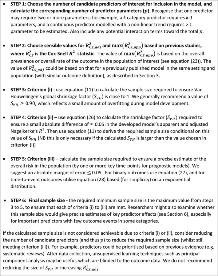
Summary of the steps involved in calculating the minimum sample size required for developing a multivariable prediction model for binary or time‐to‐event outcomes

5.1. A diagnostic prediction model for chronic Chagas disease

Our first example considers the minimum sample size required for developing a diagnostic model for predicting a binary outcome (disease: yes or no). Brasil et al developed a logistic regression model containing 14 predictor parameters for predicting the risk of having chronic Chagas disease in patients with suspected Chagas disease.46 Upon external validation in a cohort of 138 participants containing 24 with Chagas disease, the model had an estimated C statistic of 0.91 and an $R_{\mathrm{\text{Nagelkerke}}\text{\_}\mathrm{app}}^2$ of 0.48. Consider that a researcher wants to update this model and improve the predictive performance. Our sample size approach can be applied as follows.

5.1.1. Steps 1 and 2: identifying values for p, ${\mathit{R}}_{\mathbf{\text{CS}}\text{\_}\mathbf{\text{adj}}}^{\mathbf{2}}$, and $\mathbf{\text{max}}\left({\mathit{R}}_{\mathbf{\text{CS}}\text{\_}\mathbf{\text{app}}}^{\mathbf{2}}\right)$

Assume that the researcher has identified (eg, based on recent studies) 10 additional predictor parameters that they wish to add to the original model. Thus, in total, the number of predictor parameters, p , is 24. The next step is to identify a sensible value for the anticipated Cox‐Snell $R_{\text{adj}}^2$. To achieve this, we can convert the $R_{\mathrm{\text{Nagelkerke}}\text{\_}\text{app}}^2$ value for Brasil's existing model into a $R_{\text{CS}\text{\_}\text{app}}^2$ value. Assume the disease prevalence is 17.4%, as in the Brasil validation study, and use Equation (12) to calculate the log‐likelihood for the null model in Brasil's validation study

$$\ln L_{\mathrm{\text{null}}}=E\ln \left(\frac{E}{n}\right)+\left(n-E\right)\ln \left(1-\frac{E}{n}\right)=24\ln \left(\frac{24}{138}\right)+\left(138-24\right)\ln \left(1-\frac{24}{138}\right)=-63.761.$$

Hence, the $\max \left(R_{\mathrm{C}{\mathrm{S}}_{\mathrm{app}}}^2\right)=1-\exp \left(\frac{2\ln L_{\mathrm{\text{null}}}}{n}\right)=1-\exp \left(\frac{2\times -63.761}{138}\right)=0.60$. Now, we can use Equation (15) to obtain

$$R_{\mathrm{CS}\text{\_}\mathrm{app}}^2=R_{\mathrm{\text{Nagelkerke}}\text{\_}\mathrm{app}}^2\left(\max \left(R_{\mathrm{C}{\mathrm{S}}_{\mathrm{app}}}^2\right)\right)=0.48\times 0.60=0.288.$$

This apparent Cox‐Snell value of 0.288 can be directly used as an estimate of the model's $R_{\mathrm{CS}\text{\_}\mathrm{adj}}^2$, as it was obtained in a different data set to that used for model development. Therefore no adjustment is needed, because $R_{\mathrm{CS}\text{\_}\mathrm{app}}^2$= $R_{\mathrm{CS}\text{\_}\mathrm{adj}}^2$ here.

5.1.2. Step 3: criterion (i) ‐ ensuring a global shrinkage factor of 0.9

Let us assume 0.288 is a lower bound for the $R_{\mathrm{CS}\text{\_}\mathrm{adj}}^2$ of our new model. We now use Equation (11) to estimate the sample size required to ensure an expected shrinkage factor (S_VH = 0.90) conditional on a number of predictor parameters (p = 24)

$$n=\frac{p}{\left(S_{VH}-1\right)\ln \left(1-\frac{R_{\mathrm{C}{\mathrm{S}}_{\mathrm{adj}}}^2}{S_{VH}}\right)}=\frac{24}{\left(0.90-1\right)\ln \left(1-\frac{0.288}{0.90}\right)}=622.31.$$

Thus, 623 participants are required to meet criterion (i).

5.1.3. Step 4: criterion (ii) ‐ ensuring a small absolute difference in the apparent and adjusted ${\mathit{R}}_{\mathbf{\text{Nagelkerke}}}^{\mathbf{2}}$

To meet criterion (ii), we first need to calculate the shrinkage factor required to ensure a small difference of 0.05 or less in the apparent and adjusted $R_{\mathrm{\text{Nagelkerke}}}^2$. Using Equation (26), we obtain

$$S_{VH}\ge \frac{R_{\mathrm{C}{\mathrm{S}}_{\mathrm{adj}}}^2}{R_{\mathrm{C}{\mathrm{S}}_{\mathrm{adj}}}^2+\delta \max \left(R_{\mathrm{C}{\mathrm{S}}_{\mathrm{app}}}^2\right)}=\frac{0.288}{0.288+\left(0.05\times 0.60\right)}=0.906.$$

This is more stringent than the 0.90 assumed for criterion (i). Therefore, we need to reapply Equation (11) to estimate the sample size required conditional on S_VH = 0.906 (rather than 0.90)

$$n=\frac{p}{\left(S_{VH}-1\right)\ln \left(1-\frac{R_{\mathrm{C}{\mathrm{S}}_{\mathrm{adj}}}^2}{S_{VH}}\right)}=\frac{24}{\left(0.906-1\right)\ln \left(1-\frac{0.288}{0.906}\right)}=667.41.$$

Therefore, 668 subjects are required to meet criterion (ii), exceeding the 623 subjects required for criterion (i).

5.1.4. Step 5: criterion (iii) ‐ ensure precise estimate of overall risk (model intercept)

Assuming the prevalence of Chagas disease is 17.4% (as observed from the Brasil validation study), then to ensure we estimate this with a margin of error ≤ 0.05, we require (using Equation (27))

$$n={\left(\frac{1.96}{0.05}\right)}^{2}0.174\left(1-0.174\right)=220.85$$

and thus 221 subjects. This is far fewer than the sample size required to meet criteria (i) and (ii).

5.1.5. Step 6: minimum sample size that ensures all criteria are met

The largest sample size required was 668 subjects to meet criterion (ii), and so this provides the minimum sample size required for developing our new model. It corresponds to 668 × 0.174 = 116.2 events, and an EPP of 116.2/24 = 4.84, which is considerably lower than the “EPP of at least 10” rule of thumb.

5.2. A prognostic model to predict a recurrence of VTE

Our second example considers the sample size required to develop a prognostic model with a time‐to‐event outcome. Ensor et al developed a prognostic time‐to‐event model for the risk of a recurrent VTE following cessation of therapy for a first VTE.47 The sample size was 1200 participants, with a median follow‐up of 22 months, a total of 2483 person‐years of follow‐up, and 161 (13.42% of) individuals had a VTE recurrence by end of follow‐up.47 The model included predictors of age, gender, site of first clot, D‐dimer level, and the lag time from cessation of therapy until measurement of D‐dimer (often around 30 days). These predictors corresponded to six parameters in the model, which was developed using the flexible parametric survival modelling framework of Royston and Parmar48 and Royston and Lambert.49 Although Ensor's model performed well on average, the model's predicted risks did not calibrate well with the observed risks in some populations.47 Therefore, new research is needed to update and extend this model, eg, by including additional predictors. We now identify suitable sample sizes to inform such research.

5.2.1. Steps 1 and 2: identifying values for p, ${\mathit{R}}_{\mathbf{\text{CS}}\text{\_}\mathbf{\text{adj}}}^{\mathbf{2}}$ and $\mathbf{\text{max}}\left({\mathit{R}}_{\mathbf{\text{CS}}\text{\_}\mathbf{\text{app}}}^{\mathbf{2}}\right)$

Assume that there are 25 potential predictor parameters for inclusion in the new model, and thus, p = 25. We next need to identify suitable values for ${\mathit{R}}_{\mathrm{\text{CS}}\text{\_}\mathrm{\text{adj}}}^2$ and $\max \left({\mathit{R}}_{\mathrm{\text{CS}}\text{\_}\mathrm{\text{app}}}^2\right)$.

Calculating

$\mathbf{\text{max}}\left({\mathit{R}}_{\text{CS}\text{\_}\text{app}}^{\mathbf{2}}\right)$

For the Ensor model, $R_{\mathrm{CS}\text{\_}\mathrm{app}}^2$ was not reported but we should expect it to be quite small because the maximum value of $R_{\text{CS}\text{\_}\text{app}}^2$ is low. For example, assuming (for simplicity) an exponential survival model was fitted to the Ensor data, then using Equation (13), we have

$$\ln L_{\mathrm{\text{null}}}=E\ln \left(\frac{E}{T}\right)+E=161\ln \left(161/2483\right)+161=-279.47,$$

and therefore, using Equation (23),

$$\max \left(R_{\mathrm{CS}\text{\_}\mathrm{app}}^2\right)=1-\exp \left(\frac{2\ln L_{\mathrm{\text{null}}}}{n}\right)=1-\exp \left(\frac{-2\times 279.47}{1200}\right)=0.37.$$

Thus, $\max \left(R_{\mathrm{CS}\text{\_}\mathrm{app}}^2\right)$ is considerably less than 1.

Obtaining a sensible value for

${\mathit{R}}_{\text{CS}\text{\_}\text{adj}}^{\mathbf{2}}$

from the study authors

As $R_{\mathrm{CS}\text{\_}\mathrm{app}}^2$ was not reported for the Ensor model, we need to obtain it. We contacted the original authors who told us their model's $R_{\mathrm{CS}\text{\_}\mathrm{app}}^2$ was 0.056 in the development data set. Thus, let us use this value to derive $R_{\mathrm{adj}}^2$ from Equation (8). Based on Ensor's sample size of 1200, and six predictor parameters, we obtain

$$R_{\mathrm{CS}\text{\_}\mathrm{adj}}^2=S_{VH}{R}_{\mathrm{CS}\text{\_}\mathrm{app}}^2=\left(1+\frac{p}{n\ln \left(1-R_{\mathrm{CS}\text{\_}\mathrm{app}}^2\right)}\right)R_{\mathrm{CS}\text{\_}\mathrm{app}}^2=\left(1+\frac{6}{1200\ln \left(1-0.056\right)}\right)0.056=0.051.$$

Hence, when developing a new model in this field, we could assume 0.051 is a lower bound for the expected $R_{\mathrm{CS}\text{\_}\mathrm{adj}}^2$ of the new model. This corresponds to Nagelkerke's proportion variation explained of $R_{\mathrm{CS}\text{\_}\mathrm{adj}}^2/\max \left(R_{\mathrm{CS}\text{\_}\mathrm{app}}^2\right)\approx$ 0.051/0.37 = 0.14 (or 14%).

Calculating a sensible value for

${\mathit{R}}_{\mathbf{\text{CS}}\text{\_}\mathbf{\text{adj}}}^{\mathbf{2}}$

from other reported information

For illustration, we also consider how $R_{\mathrm{CS}\text{\_}\mathrm{app}}^2$ could have been estimated indirectly from other available information. The model's reported C statistic was 0.69, and so we can use Equation (22) to predict the corresponding D statistic

$$D=5.50\left(C-0.5\right)+10.26{\left(C-0.5\right)}^3=5.50\left(0.69-0.5\right)+10.26{\left(0.69-0.5\right)}^3=1.115.$$

The corresponding $R_{D\text{\_}\mathrm{app}}^2$ can be derived from Equation (21)

$$R_{D\text{\_}\mathrm{app}}^2=\frac{\frac{\pi }{8}{D}^2}{\frac{{\pi }^2}{6}+\frac{\pi }{8}{D}^2}=\frac{\frac{\pi }{8}{1.115}^2}{\frac{{\pi }^2}{6}+\frac{\pi }{8}{1.115}^2}=0.229.$$

Taking $R_{D\text{\_}\mathrm{app}}^2$ as a proxy for $R_{\mathrm{\text{Royston}}\text{\_}\mathrm{app}}^2$, we can then use Equation (20) to obtain

$$R_{\mathrm{O}\text{'}\mathrm{\text{Quigley}}\text{\_}\mathrm{app}}^2=\frac{-\frac{{\pi }^2}{6}{R}_{\mathrm{\text{Royston}}\text{\_}\mathrm{app}}^2}{\left(1-\frac{{\pi }^2}{6}\right)R_{\mathrm{\text{Royston}}\text{\_}\mathrm{app}}^2-1}=\frac{-\frac{{\pi }^2}{6}0.229}{\left(1-\frac{{\pi }^2}{6}\right)0.229-1}=0.328.$$

Next, we can use $R_{\mathrm{O}\text{'}\mathrm{\text{Quigley}}\text{\_}\mathrm{app}}^2$ and the number of reported events (E = 161) to derive the LR statistic from Equation (18)

$$\mathrm{LR}=-E\ln \left(1-R_{{\mathrm{O}}^{\text{'}}\mathrm{\text{Quigle}}{\mathrm{y}}_{\mathrm{app}}}^2\right)=-161\ln \left(1-0.328\right)=64.05.$$

Using Equation (6), this corresponds to

$$R_{\mathrm{CS}\text{\_}\mathrm{app}}^2=1-\exp \left(\frac{-\mathrm{LR}}{n}\right)=1-\exp \left(\frac{-64.05}{1200}\right)=0.052.$$

Thus, based on using the reported C statistic, an indirect estimate of the $R_{\mathrm{CS}\text{\_}\mathrm{app}}^2$ is 0.052 for the Ensor model. This is reassuringly close to the estimate of 0.056 provided directly by the study authors.

5.2.2. Step 3: criterion (i) ‐ ensuring a global shrinkage factor of 0.9

Equation (11) can now be applied to derive the required sample size to meet criterion (i). Using an $R_{\mathrm{CS}\text{\_}\mathrm{adj}}^2$ of 0.051, for a model with 25 predictor parameters and a targeted expected shrinkage of 0.9, the sample size required is

$$n=\frac{p}{\left(S_{VH}-1\right)\ln \left(1-\frac{R_{\mathrm{CS}\text{\_}\mathrm{adj}}^2}{S_{VH}}\right)}=\frac{25}{\left(0.9-1\right)\ln \left(1-\frac{0.051}{0.9}\right)}=4285.5$$

and thus 4286 participants.

5.2.3. Step 4: criterion (ii) ‐ ensuring a small absolute difference in the apparent and adjusted ${\mathit{R}}_{\mathbf{\text{Nagelkerke}}}^{\mathbf{2}}$

To meet criterion (ii), we first need to calculate the shrinkage factor required to ensure a small difference of 0.05 or less in the apparent and adjusted $R_{\mathrm{\text{Nagelkerke}}}^2$. Recall, assuming an exponential model for simplicity, we calculated that the $\text{max}\left(R_{\mathrm{C}{\mathrm{S}}_{\text{app}}}^2\right)=0.37$. Then, using Equation (26), we obtain

$$S_{VH}\ge \frac{R_{\mathrm{C}{\mathrm{S}}_{\mathrm{adj}}}^2}{R_{\mathrm{C}{\mathrm{S}}_{\mathrm{adj}}}^2+\delta \max \left(R_{\mathrm{C}{\mathrm{S}}_{\mathrm{app}}}^2\right)}=\frac{0.051}{0.051+\left(0.05\times 0.37\right)}=0.73.$$

This is less stringent than the 0.90 assumed for criterion (i), and so no further sample size calculation is required to meet criterion (ii).

5.2.4. Step 5: criterion (iii) ‐ ensure precise estimate of overall risk

Assuming a simple exponential model, we can check the width of the confidence interval for the overall risk at a particular time point based on the sample size identified, using the approach outlined in Section 4.2. Ensor et al47 reported an overall VTE recurrence rate of 161/2483 = 0.065, with an average follow‐up of 2.07 years. Therefore, assuming λ is 0.065 in our new study, and that a predicted risk at 2 years is of key interest, an exponential survival model would give the cumulative incidence of F(2) = 1 −  exp (−0.065 × 2) = 0.122. Based on the calculated sample size of 4286 participants from criterion (i), and thus an estimated 4286×2.07 = 8872 person‐years of follow‐up, the 95% confidence interval would be

$$1-\exp \left(-\left(\widehat{\lambda }\pm 1.96\sqrt{\frac{\widehat{\lambda }}{T}}\right)t\right)=1-\exp \left(-\left(0.065\pm 1.96\sqrt{\frac{0.065}{8872}}\right)2\right)=0.113\text{to}0.131.$$

This is reassuringly narrow, and satisfies Equation (28) as both the lower and upper bounds are well within an error of 0.05 of the true value of 0.122.

5.2.5. Step 6: minimum sample size that ensures all criteria are met

The largest sample size required was 4286 participants to meet criterion (i), which therefore provides the minimum sample size required for developing our new model. This assumes the new cohort will have a similar follow‐up, censoring rate, and event rate to that reported by Ensor et al, where the mean follow‐up per person was 2.07 years, 13.42% of individuals had a VTE recurrence by end of follow‐up, and the event rate was 0.065.47

Then, the required 4286 participants corresponds to about 4286 × 2.07 = 8872 person‐years of follow‐up, and 8872 × 0.065 ≈ 577 outcome events, and thus an EPP of 577/25 ≈ 23. This is over twice the “EPP of at least 10” rule of thumb. Figure 2 shows that an EPP of 10 only ensures a shrinkage factor of 0.79, which would reflect relatively large overfitting.

Figure 2.

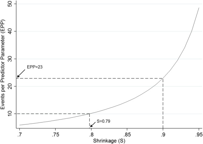
Events per predictor parameter required to achieve various expected shrinkage (S_VH) values for a new prediction model of venous thromboembolism recurrence risk with an assumed $R_{\mathrm{CS}\text{\_}\mathrm{adj}}^2$ of 0.051 [Colour figure can be viewed at wileyonlinelibrary.com]

5.2.6. What if the sample size is not achievable?

If a researcher was restricted in their total sample size, for example, by the time and cost of a new cohort study, then a sample size of 4286 may not be practical. In this situation, we do not recommend reducing sample size by decreasing S_C below 0.9 (as this would reflect larger overfitting) or by assuming a larger $R_{\mathrm{CS}\text{\_}\mathrm{adj}}^2$ value (as this is anticonservative for criterion (i)). Rather, to ensure an S_VH of 0.9 (ie, an expected shrinkage of 10%), the researcher should lower p by reducing the number of candidate predictors. For example, predictors could be prioritised based on previous evidence (eg, systematic reviews). After data collection, unsupervised learning techniques such as principal component analysis may be useful, which are blinded to the outcome data. Figure 3 shows how changing p changes the required sample size to meet criterion (i). For example, if a researcher was restricted to a sample size of about 2000 participants, then they would need to reduce p to 12 to ensure an expected shrinkage of 0.90. This is because, for an S_VH of 0.9 and $R_{\mathrm{CS}\text{\_}\mathrm{adj}}^2$ of 0.051, the sample size required is

$$n=\frac{p}{\left(S_{VH}-1\right)\ln \left(1-\frac{R_{\mathrm{CS}\text{\_}\mathrm{adj}}^2}{S_{VH}}\right)}=\frac{12}{\left(0.9-1\right)\ln \left(1-\frac{0.051}{0.9}\right)}=2057$$

and so now close to 2000. Figure 3 also shows how larger values of S_VH require larger sample sizes; in particular, the increase in sample size required is substantial when moving from S_VH of 0.90 to 0.95. Values of S_VH < 0.9 lead to lower sample sizes, but come at the cost of larger expected overfitting, and so are not recommended. Therefore, targeting a value of S_VH of 0.9 would seem a pragmatic choice.

Figure 3.

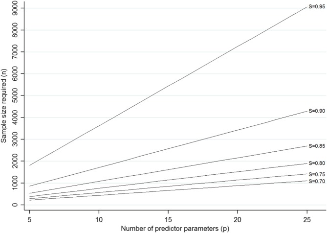
Sample size required (based on Equation (11)) for a particular number of predictor parameters (p) to achieve a particular value of expected shrinkage (S_VH), for a new prediction model of venous thromboembolism recurrence risk with an assumed $R_{\mathrm{CS}\text{\_}\mathrm{adj}}^2$ of 0.051 [Colour figure can be viewed at wileyonlinelibrary.com]

6. POTENTIAL ADDITIONAL CRITERION: PRECISE ESTIMATES OF PREDICTOR EFFECTS

Ideally, predictions should also be precise across the entire spectrum of predicted values, not just at the mean. This is challenging to achieve, but is helped by ensuring the sample size will give precise estimates of the effects of key predictors;50 hence, this may form a further criterion for researchers to check (ie, in addition to criteria (i) to (iii)). Briefly, for a particular predictor of a binary or time‐to‐event outcome, the sample size required to precisely estimate its association with the outcome (ie, an odds ratio or hazard ratio) depends on the assumed magnitude of this effect, the variability of the predictor's values across subjects, the predictor's correlation with other predictors in the model, and the overall outcome proportion in the study.51, 52, 53 Ideally, we want to ensure a sample size that gives a precise confidence interval around the predictor's effect estimate.54 However, this is taxing, as closed‐form solutions for the variance of adjusted log odds ratio or hazard ratios, from logistic and Cox regression, respectively, are nontrivial. One solution is to use simulation‐based evaluations.54, 55 However, perhaps a more practical option is to utilise readily available power‐based sample size calculations that calculate the sample size required to detect (based on statistical significance) a predictor's effect for a chosen type I error level (eg, 0.05) and power.51, 52, 53, 56 As such sample size calculations are likely to be less stringent than those based on confidence interval width (especially for predictors with large effect sizes), we might use a high power, say of 95%, in the calculation.

Checking sample size for predictor effects will be laborious with many predictors, and so it may be practical to focus on the subset of key predictors with smallest variance of their values, as these predictors will have the least precision. In particular, when there are important categorical predictors but with few subjects and/or outcome events in some categories, substantially larger sample sizes may be needed to avoid separation issues (ie, no event or nonevents in some categories).57 In addition, any predictors whose effect is small (and thus harder to detect), but still important, may warrant special attention.

For example, returning to the VTE prediction model from Section 5.2, a key predictor in the original model by Ensor et al was age,47 with an adjusted log hazard ratio of −0.0105. Although this is close to zero, as age is on a continuous scale, the impact of age on outcome risk is potentially large; for example, it corresponds to an adjusted hazard ratio of 0.66 comparing two individuals aged 40 years apart. Based on the results presented by Ensor et al,47 the standard deviation of age was 15.21 and the overall outcome occurrence by end of follow‐up was 13.5%. Based on these values, and assuming other included predictors explain 20% of the variation in age, then the sample size approach of Hsieh and Lavori52 suggests 4718 subjects are required to have 95% power to detect a prognostic effect for age. This is larger than the 4286 subjects required to meet criterion (i), and so, to be extra stringent beyond criteria (i) to (iii), the researcher might raise the recommended sample size to 4718 subjects, if possible.

7. DISCUSSION

Sample size calculations for prediction models of binary and time‐to‐event outcomes are typically based on blanket rules of thumb, such as at least 10 EPP, which generates much debate and criticism.14, 16, 57 In this article, building on our related work for linear regression,10 we have proposed an alternative approach that identifies the sample size, events and EPP required to meet three key criteria, which minimise overfitting whilst ensuring precise estimates of overall outcome risk. Criterion (i) aims to ensure the optimism of predictor effect estimates is small, as defined by a global shrinkage factor of ≥ 0.9. This idea extends the work of Harrell who suggests that, after a model is developed, if the shrinkage estimate “falls below 0.9, for example, we may be concerned with the lack of calibration the model may experience on new data.”15 Our premise is the same, except we focused on calculating the expected shrinkage before data collection, to inform sample size calculations for a new study. Criterion (ii) extends this idea to ensure the optimism is small on the $R_{\mathrm{\text{Nagelkerke}}}^2$ scale, such that there is a difference of ≤ 5% in the apparent and adjusted percentage of variation explained by the model. Lastly, criterion (iii) ensures the sample size will precisely estimate the overall outcome risk, which is fundamental.

By utilising the model's anticipated Cox‐Snell R², the sample size calculations are essentially tailored to the model and setting at hand, because the Cox‐Snell R² reflects many factors including the outcome proportion (ie, outcome prevalence or cumulative incidence) and the overall fit (performance) of the model. It therefore better reflects the trait of a particular model and setting at hand rather than a blanket EPP rule.16 In our examples, the sample sizes required often differed considerably from an EPP of 10, reinforcing the idea that this rule is too simplistic.57 Indeed, the required EPP was much higher (23) in our second example than our first (4.8), illustrating the problem with a blanket EPP rule trying to cover all situations.14, 16, 17, 18

Section 3 also showed how to obtain a realistic value for Cox‐Snell R² based on previous models to make our proposal more achievable in practice. If no previous prediction model exists for the outcome and setting of interest, then information might be used from studies in a related setting or using a different but similar outcome definition or time points to those intended for the new model. Information can also be borrowed from predictor finding studies (eg, studies aiming to estimate the prognostic effect of a particular predictor adjusted for other predictors58). Typically, these studies apply multivariable modelling, and although mainly focused on predictor effect estimates, they often report the C statistic and pseudo‐R² values.

Further research is needed to help researchers when there are no existing studies or information to identify a sensible value of the expected Cox‐Snell R². Medical diagnosis and prediction of health‐related outcomes are, generally speaking, low signal‐to‐noise ratio situations. It is not uncommon in these situations to see $R_{\mathrm{\text{Nagelkerke}}}^2$ values in the 0.1 to 0.2 range. Therefore, in the absence of any other information, we suggest that sample sizes be derived assuming the value of $R_{\mathrm{CS}\text{\_}\mathrm{adj}}^2$ corresponds to an $R_{\mathrm{\text{Nagelkerke}}}^2$ of 0.15 (ie, $\frac{R_{\mathrm{C}{\mathrm{S}}_{\mathrm{adj}}}^2}{\max \left(R_{\mathrm{C}{\mathrm{S}}_{\mathrm{adj}}}^2\right)}=0.15$). An exception is when predictors include “direct” (mechanistic) measurements, such as including the baseline version of the binary or ordinal outcome (eg, including smoking status at baseline when predicting smoking status at 1 year), or direct measures of the processes involved (eg, including physiologic function of patients in intensive care when predicting risk of death within 48 hours). Then, in this special situation, an $R_{\mathrm{\text{Nagelkerke}}}^2=0.5$may be a more appropriate default choice.

The rule of having an EPP of at least 10 stems from limited simulation studies examining the bias and precision of predictor effects in the prediction model.11, 12, 13 Jinks et al41 alternatively developed sample size formulae for a time‐to‐event prediction model based on the D statistic.40 They suggest to predefine the D statistic that would be expected, and then, based on a desired significance or confidence interval width, their formulae provide the number of events required to achieve this. However, their method does not account for the number of candidate predictors and does not consider the potential for overfitting when developing a model. Our sample size calculations address this, and are meant to be used before any data collection. In situations where a development data set is already available, containing a specific number of participants and predictors, our criteria could be used to identify whether a reduction in the number of predictors is needed before starting model development. Indeed, Harrell already illustrated this concept by using the shrinkage estimate from the full model (including all predictors) to gauge whether the number of predictors should be reduced via data reduction techniques.15 Ideally, this should be done blind to the estimated predictor effects (ie, just calculate the shrinkage factor for the full model, but do not observe the predictor effect estimates and associated p‐values), as otherwise decisions about predictor inclusion are influenced by a “quick look” at the effect estimates from the full model results. Similarly, when planning to use a predictor selection method (such as backwards selection) during model development, researchers should define p as the total number of parameters due to all predictors considered (screened), and not just the subset that are included in the final model.59 As Harrell notes,15 the value of p should be honest.

Section 6 also highlighted the potential additional requirement to ensure precise estimates of key predictor effects. In particular, special attention may be given to those predictors with strong predictive value (and thus most influential to the predicted outcome risk), especially if the variance in their values is small, or when events or nonevents in some categories of the predictor are rare, as this leads to larger sample sizes. For example, van Smeden et al highlighted that “separation” between events and nonevents is an important consideration toward the required sample size, which occurs when a single predictor (or a linear combination of multiple predictors) perfectly separates all events from all nonevents, and thus causes estimation difficulties.57 This may lead to substantially larger EPP to resolve the issue (eg, so that all categories of a predictor have both events and nonevents). For such reasons, we labelled our criteria (i) to (iii) proposal as the “minimum” sample size required.

Further research should identify how our sample size criteria relates to that of the work of van Smeden et al, who focused on sample size in regards to the mean squared error in predictions from the model.60 Specifically, they use simulation to evaluate the characteristics that influence the mean squared prediction error of a logistic model, and identify that the outcome proportion and number of predictors are important,60 in addition to total sample size. This leads to a sample size equation to minimise root mean‐squared prediction error in a new model development study. Harrell also suggested using simulation to inform sample size, and illustrates this for a logistic regression model with a single predictor.15 For example, one could simulate a very large dataset from an assumed prediction model, and quantify the mean square (prediction) error and mean absolute (prediction) error of a model developed from this data set. Then, repeat this process each time removing an individual at random, until a sample size is identified below which the mean squared (prediction) error is unacceptable.

In summary, we have proposed criteria for identifying the minimum sample size required when developing a prediction model for binary or time‐to‐event outcomes. We hope this, and our related paper,10 encourages researchers to move away from rules of thumb, and to rather focus on attaining sample sizes that minimise overfitting and ensure precise estimates of overall risk within the model and setting of interest. We are currently writing software modules to implement the approach.

Riley RD, Snell KIE, Ensor J, et al. Minimum sample size for developing a multivariable prediction model: PART II ‐ binary and time‐to‐event outcomes. Statistics in Medicine. 2019;38:1276–1296. 10.1002/sim.7992

REFERENCES

- 1. Steyerberg EW. Clinical Prediction Models: A Practical Approach to Development, Validation, and Updating. New York, NY: Springer Science+Business Media; 2009. [Google Scholar]
- 2. Royston P, Moons KG, Altman DG, Vergouwe Y. Prognosis and prognostic research: developing a prognostic model. Br Med J. 2009;338:1373‐1377. 10.1136/bmj.b604 [DOI] [PubMed] [Google Scholar]
- 3. Steyerberg EW, Moons KG, van der Windt DA, et al. Prognosis research strategy (PROGRESS) 3: prognostic model research. PLoS Med. 2013;10(2):e1001381. [DOI] [PMC free article] [PubMed] [Google Scholar]
- 4. Wells PS, Anderson DR, Rodger M, et al. Derivation of a simple clinical model to categorize patients probability of pulmonary embolism: increasing the models utility with the SimpliRED D‐dimer. Thromb Haemost. 2000;83(3):416‐420. [PubMed] [Google Scholar]
- 5. Wells PS, Anderson DR, Bormanis J, et al. Value of assessment of pretest probability of deep‐vein thrombosis in clinical management. Lancet. 1997;350(9094):1795‐1798. [DOI] [PubMed] [Google Scholar]
- 6. Anderson KM, Odell PM, Wilson PW, Kannel WB. Cardiovascular disease risk profiles. Am Heart J. 1991;121(1 Pt 2):293‐298. [DOI] [PubMed] [Google Scholar]
- 7. Hippisley‐Cox J, Coupland C, Vinogradova Y, et al. Predicting cardiovascular risk in England and Wales: prospective derivation and validation of QRISK2. BMJ. 2008;336(7659):1475‐1482. [DOI] [PMC free article] [PubMed] [Google Scholar]
- 8. Haybittle JL, Blamey RW, Elston CW, et al. A prognostic index in primary breast cancer. Br J Cancer. 1982;45(3):361‐366. [DOI] [PMC free article] [PubMed] [Google Scholar]
- 9. Galea MH, Blamey RW, Elston CE, Ellis IO. The Nottingham prognostic index in primary breast cancer. Breast Cancer Res Treat. 1992;22(3):207‐219. [DOI] [PubMed] [Google Scholar]