Geodesic Lagrangian Monte Carlo over the space of positive definite matrices: with application to Bayesian spectral density estimation

Abstract

We present geodesic Lagrangian Monte Carlo, an extension of Hamiltonian Monte Carlo for sampling from posterior distributions defined on general Riemannian manifolds. We apply this new algorithm to Bayesian inference on symmetric or Hermitian positive definite matrices. To do so, we exploit the Riemannian structure induced by Cartan’s canonical metric. The geodesics that correspond to this metric are available in closed-form and—within the context of Lagrangian Monte Carlo—provide a principled way to travel around the space of positive definite matrices. Our method improves Bayesian inference on such matrices by allowing for a broad range of priors, so we are not limited to conjugate priors only. In the context of spectral density estimation, we use the (non-conjugate) complex reference prior as an example modeling option made available by the algorithm. Results based on simulated and real-world multivariate time series are presented in this context, and future directions are outlined.

1. Introduction

In this paper, we introduce geodesic Lagrangian Monte Carlo (gLMC), a methodology for Bayesian inference on a broad class of Riemannian manifolds. We illustrate this general methodology using the space of positive definite (PD) matrices as a concrete example. The resulting algorithms allow for direct inference on the space of PD matrices and are thus the first of their kind. As a result, gLMC facilitates better prior elicitation of covariance matrices by negating the need for conjugate priors and avoiding difficult-to-interpret transformations on variables of interest.

In statistics, positive definite matrices primarily appear as covariance matrices parameterizing the multivariate Gaussian model. This model is the workhorse of modern statistics and machine learning: linear regression, probabilistic principal components analysis, Gaussian Markov random fields, spectral density estimation, and Gaussian process models all rely on the multivariate Gaussian distribution. The d-dimensional Gaussian distribution is completely specified by a mean vector μ and a covariance matrix $\sum \text{in}\hspace{0.17em}{S}_d^{+},$ the space of d-by-d PD matrices. By imposing different structures on the covariance matrix, one can create different models. In some cases, it is possible to parameterize the covariance matrices in terms of a small number of parameters. However, learning of the unstructured covariance matrices, usually involved in inference on a large number of parameters, has remained as an issue. The conjugate Gaussian inverse-Wishart model has known deficiencies [1]. Outside of non-linear parameterizations of the Cholesky decomposition or matrix logarithm, there has not yet been a way to perform Bayesian inference directly on the space of PD matrices with flexible prior specifications using unstructured covariance matrices.

In this most general context the difficulty is in sampling from a posterior distribution on an abstract, high-dimensional manifold with boundary. It has not been clear how to propose moves from point to point within (and without leaving) this space. Our method takes advantage of the intrinsic, Riemannian geometry on the space of PD matrices. This space is incomplete under the Euclidean metric: following a straight trajectory will often result in matrices that are no longer positive definite. The space is, however, geodesically complete under the canonical metric: no matter how far the sampler travels along any geodesic, it never leaves the space of PD matrices. Intuitively, we redefine ‘straight line’ in a way that precludes leaving the set of interest. Moreover, the metric-induced geodesics provide a natural way to traverse the space of PD matrices, and these geodesics fit nicely with recent advances in Hamiltonian Monte Carlo on manifolds [2–4].

To this end, we use geodesic Lagrangian Monte Carlo (gLMC), which belongs to a growing class of Hamiltonian Monte Carlo algorithms. Hamiltonian Monte Carlo (HMC) provides an intelligent, partially deterministic method for moving around the parameter space while leaving the target distribution invariant. New Markov states are generated by numerically integrating a Hamiltonian system while Metropolis-Hastings steps account for the numerical error [5]. Riemannian manifold Hamiltonian Monte Carlo (RMHMC) adapts the proposal path by incorporating second-order information in the form of a Riemannian metric tensor [2]. Lagrangian Monte Carlo (LMC) builds on RMHMC by using a random velocity in place of RMHMC’s random momentum. LMC’s explicit integrator is no longer volume preserving; it therefore requires Jacobian corrections for each accept-reject step [6]. The embedding geodesic Monte Carlo (egMC) [3] is able to take the geometry of the parameter space into account while avoiding implicit integration by splitting the Hamiltonian [7] into a Euclidean and a geodesic component. Unfortunately, egMC is not applicable when a manifold’s Riemannian embedding is unknown. gLMC, on the other hand, efficiently uses the same split Hamiltonian formulation as egMC but does not require an explicit Riemannian embedding [See 4, for example]. This last fact makes gLMC an ideal candidate for Bayesian inference on the space of PD matrices.

gLMC allows us to treat the entire covariance matrix as one would treat any other model parameters. We are no longer restricted to use a conjugate prior distribution or to specify a low-rank structure. We illustrate applications of gLMC for PD matrices using both simulated and real-world data. First, we show that gLMC provides the same empirical results as the closed-form solution for the conjugate Gaussian inverse-Wishart model. After this, we focus on applying gLMC for Hermitian PD matrices to multivariate spectral density estimation and compare the results obtained from two different prior specifications: the inverse-Wishart prior and the complex reference prior. Then, we obtain credible intervals for the squared coherences (see Section 2) of simulated vector auto-regressive time series for which the spectral density matrix is known. Finally, we apply gLMC to learn the spectral density matrix associated with multivariate local field potentials (LFPs).

The contributions of this paper are as follows:

• gLMC, an MCMC methodology for Bayesian inference on general Riemannian manifolds, is proposed;

• to illustrate the general methodology, we provide a detailed description of gLMC on the spaces of symmetric and Hermitian PD matrices;

• for classical statisticians, the paper serves as a brief introduction to spectral density estimation and its Bayesian approach;

• the proposed algorithms are applied to Bayesian inference on (real and complex) covariance matrices based on simulated and real-world data and using a number of different prior specifications.

It should be noted that the proposed method is useful for generating samples from the posterior distribution of interest and not just a point estimate. The proposed method is for full inference of a posterior distribution defined directly over the space of PD matrices without limiting ourselves to conjugate priors, as such, is the first of its kind.

That said, it is sometimes sufficient for the scientist to obtain a point estimate of the covariance or spectral density matrix. In this context, regularization of the estimate is often advantageous. Regularization approaches may be interpreted as Bayesian and their corresponding point estimates are interpreted as maximum a posteriori (MAP) estimates. See [8] for a statistically minded survey of covariance estimation and regularization, and see [9] for a state-of-science approach to point estimation in signal processing applications.

The rest of the paper is outlined thus: in Section 2, we provide motivation for our approach in the form of a brief introduction to spectral density estimation for multivariate time series; in Section 3, we define PD matrices and show how the space of PD (symmetric or Hermitian) matrices comprises a Riemannian manifold; in Section 4, we present the gLMC methodology for Bayesian inference on general Riemannian manifolds; in Section 5, we detail gLMC on the spaces of symmetric and Hermitian PD matrices; in Section 6, we introduce the reader to common proper and improper priors for covariance matrices; in Section 7, we present empirical results based on simulated and real-world data.

2. Motivation: learning the spectral density matrix

Given a stationary multivariate time series $y\left(t\right)={\left(y_1\left(t\right),\mathrm{...},y_d\left(t\right)\right)}^{\text{T}}\in \hspace{0.17em}\hspace{0.17em}{ℝ}^d,t=1,\mathrm{...},T,$ one often wants to characterize the dependencies between vector elements through time. There are multiple ways to define such dependencies, and these definitions feature either the time series directly or the Fourier-transformed series in the frequency domain. In the time domain, one characterization of dependence is provided by the lagged variance-covariance matrix Γ_ℓ. In terms of lag _ℓ, this is written

$${\text{Γ}}_{\ell }=\text{Cov}\left(y\left(t\right),y\left(t-\ell \right)\right)=\text{E}\left(\left(y\left(t\right)-\mu \right){\left(y\left(t-\ell \right)-\mu \right)}^T\right).$$ (1)

Note that Γ_ℓ and μ are invariant over time by stationarity. If the scientist has a reason to suspect that a certain lag _ℓ is important a priori, then Γ_ℓ can be a useful measure. On the other hand, it is often more scientifically tractable to think in terms of frequencies rather than lags. In neuroscience, for example, one might hypothesize that two brain regions have ‘correlated’ activity during the performance of a specific task, but this co-activity may be too complex to describe in terms of a simple lagged relationship. The spectral density approach lends itself naturally to this kind of question. For a full discussion, see [10].

The power spectral density matrix is the Fourier transform of Γ_ℓ:

$$\Sigma \left(\omega \right)=\sum _{\ell =-\infty }^{\infty }{\Gamma }_{\ell }\exp \left(-i2\pi \omega \ell \right).$$ (2)

Σ(ω) is a Hermitian PD matrix. A Hermitian matrix M is a complex valued matrix satisfying $M^H={\overline{M}}^T=M$, where $\overline{(\cdot )}$ denotes taking the complex conjugate. A Hermitian matrix M is defined to be PD if $z^{H}Mz>0,{\forall }_z\in {ℂ}^d\backslash \left\{0\right\}$.

A diagonal element Σ_ii(ω) is called the auto-spectrum of y_i(t) at frequency ω, and an off-diagonal element Σ_ij(ω), i ≠ j is the cross-spectrum of y_i(t) and y_j(t) at frequency ω. The squared coherence is given by

$${\rho }_{ij}^2\left(\omega \right)=\frac{{\left|{\sum }_{ij}\left(\omega \right)\right|}^2}{{\sum }_{ii}\left(\omega \right){\sum }_{jj}\left(\omega \right)},$$ (3)

where | · | denotes the complex modulus. There are a number of ways to estimate the spectral density matrix and, hence, the matrix of squared coherences. In this paper, we use theWhittle likelihood approximation [11].We model the discrete Fourier transformed time series $Y\left({\omega }_k\right)\in {ℂ}^d$ as following a (circularly-symmetric) complex multivariate Gaussian distribution:

$$Y\left({\omega }_k\right)\stackrel{ind}{\sim }{\text{CN}}_d\left(0,\Sigma \left({\omega }_k\right)\right),$$ (4)

where, for ${\omega }_k=\frac{k}{T}$ and $k=-\left(\frac{T}{2}-1\right),\dots ,\frac{T}{2}$,

$$Y\left({\omega }_k\right)=\frac{1}{\sqrt{T}}\sum _{t=1}^{T}y\left(t\right)\hspace{0.17em}\hspace{0.17em}\exp \left(-i2\pi {\omega }_{k}t\right).$$ (5)

Three assumptions are made here. First, we assume that the Y (ω_k)s are exactly Gaussian: this is true when the y(t) follow any Gaussian process. Moreover, if y(t) follow a linear process, then the Y (ω_k) are asymptotically Gaussian as T goes to infinity [12]. Second, we assume that for ω_k ≠ ω_k′ , Y (ω_k) and Y (ω_k′) are independent, whereas [12] show that they are asymptotically uncorrelated. Third, we assume that Σ(·) is approximately piecewise constant across frequency bands, and take all Y (ω_k) to be approximately i.i.d. within a small enough frequency band. For example, if we are interested in the alpha band of neural oscillations ranging from 7.5 to 12.5 Hz, then we model

$$Y\left({\omega }_k\right)\stackrel{iid}{\sim }{\text{CN}}_d\left(0,{\Sigma }_{\alpha }\right),$$ (6)

where Σ_α denotes the spectral density matrix shared by the entire band. For a recent use of the approximately piecewise constant assumption, see [13], where the spectrum is represented as a sum of unique AR(2) spectra, with each of the AR(2) capturing distinct frequency bands.

Thus, having obtained samples Y (ω) from a fixed frequency band, we will use gLMC over Hermitian PD matrices to perform inference on Σ. The posterior samples of Σ automatically provide samples for the distributions of the squared coherences, which can in turn elucidate dependencies between the univariate time series. Before discussing gLMC for PD matrices, we establish necessary facts regarding the space of positive definite matrices.

3. The space of positive definite matrices²

Let S_d(ℂ) denote the space of d×d Hermitian matrices, and $S_d^{+}\left(ℂ\right)$ denote its subspace of PD matrices. The space of Hermitian PD matrices, $S_d^{+}\left(ℂ\right)$, may be written as a quotient space GL(d,ℂ)/U(d) of the complex general linear group GL(d,ℂ) and the unitary group U(d). The general linear group is the smooth manifold for which every point is a matrix with non-zero determinant. The unitary group is the space of all complex matrices U satisfying U^HU = UU^H = I. This quotient space representation is rooted in the fact that every PD matrix may be written as the product Σ = GG^H = GUU^HG^H for a unique G ∈ GL(d, ℂ) and any arbitrary unitary matrix U ∈ U(d). For the convenience of exposition, we drop the dependence on ℂ of symbols in the following of this section. Related references are [14–16].

$S_d^{+}$ is a homogeneous space with respect to the general linear group: this means that the group acts transitively on the $S_d^{+}$. Here the group action is given by conjugation:

$$G^{*}\Sigma =G\Sigma G^H.$$ (7)

For any ${\Sigma }_1,{\Sigma }_2\in S_d^{+}$, it simply takes the composition ${\Sigma }_1^{1/2\ast }\hspace{0.17em}○\hspace{0.17em}\hspace{0.17em}{\Sigma }_1^{-1/2\ast }$ to transform Σ₁ into Σ₂:

$${\Sigma }_2^{1/2\ast }\hspace{0.17em}○\hspace{0.17em}\hspace{0.17em}{\Sigma }_1^{-1/2\ast }\hspace{0.17em}{\Sigma }_1={\Sigma }_2^{1/2\ast }\left({\Sigma }_1^{-1/2}{\Sigma }_1{\Sigma }_1^{-1/2}\right)={\Sigma }_2^{1/2}I{\Sigma }_2^{1/2}={\Sigma }_2.$$ (8)

The space of Hermitian matrices, S_d, happens to be the tangent space to the space of Hermitian PD matrices at the identity, denoted as $T_{Id}{S}_d^{+}$, that is, $T_{Id}{S}_d^{+}=S_d$. The action

$${\Sigma }^{1/2\ast }:V\mapsto {\Sigma }^{1/2}V{\Sigma }^{1/2}$$ (9)

translates vector $V\in T_{Id}{S}_d^{+}$ to its corresponding vector in $T_{\Sigma }{S}_d^{+}$, the tangent space to the space of PD matrices at point Σ.

Élie Cartan constructed a natural Riemannian metric g(·,·) on the tangent bundle $T{S}_d^{+}$ that is invariant under group action (7). For two vectors $V_1,V_2\in T_{Id}{S}_d^{+}$ , the metric is given by

$$gI\left(V_1,V_2\right)=\text{tr}\left(V_1{V}_2\right).$$ (10)

In this way the space of PD matrices is isometric to Euclidean space (equipped with the Frobenius norm) at the identity. Next define the metric at any arbitrary point Σ to be

$$g\Sigma \left(V_1,V_2\right)=\text{tr}\left({\Sigma }^{-1}{V}_1{\Sigma }^{-1}{V}_2\right)$$ (11)

It is easy to check that gI (V₁, V₂) = gΣ(Σ^1/2*V₁,Σ^1/2*V₂) and so Σ^1/2* is a Riemannian isometry on $S_d^{+}$.

Two geometric quantities are required for our purposes: the Riemannian metric tensor and its corresponding geodesic flow, specified by a starting point and an initial velocity vector. The computational details involving the metric tensor are presented in Section 5. Here we present the closed form solution for the geodesic flow as found in [14]. $S_d^{+}$ is an affine symmetric space [17]. As such the geodesics under the invariant metric are generated by the one-parameter subgroups of the acting Lie group [14, 16]. These one-parameter subgroups are given by the group exponential map which, at the identity, is given by the matrix exponential exp tG. In order to calculate the unique geodesic curve with starting position Σ(0) and initial velocity V (0), all one needs is to translate the velocity to the identity, compute the matrix exponential, and translate it back to the point of interest. In sum, the geodesic is given by

$$\Sigma \left(t\right)={\exp }_{\Sigma }tV\left(0\right)=\Sigma {\left(0\right)}^{1/2}\exp \left(t\Sigma {\left(0\right)}^{-1/2}V\left(0\right)\Sigma {\left(0\right)}^{-1/2}\right)\Sigma {\left(0\right)}^{1/2}.$$ (12)

The corresponding flow on the tangent bundle will also be useful. This is obtained by taking the derivative with respect to t:

$$\begin{array}{l}V\left(t\right)=\dot{\Sigma }\left(t\right)=\frac{d}{dt}{\exp }_{\Sigma }tV\left(0\right)\\ \hspace{0.17em}\hspace{0.17em}\hspace{0.17em}\hspace{0.17em}\hspace{0.17em}\hspace{0.17em}\hspace{0.17em}\hspace{0.17em}\hspace{0.17em}\hspace{0.17em}\hspace{0.17em}=V\left(0\right)\Sigma {\left(0\right)}^{-1/2}\exp \left(t\Sigma {\left(0\right)}^{-1/2}V\left(0\right)\Sigma {\left(0\right)}^{-1/2}\right)\Sigma {\left(0\right)}^{-1/2}.\end{array}$$ (13)

For a Lie group, the exponential map (on which the above formula is based) is a local diffeomorphism between the tangent space at a point on the manifold and the manifold itself. Given a tangent vector V at Σ, exp_Σ V is a point on the manifold. Incidentally, for the spaces of PD matrices, this diffeomorphism is global. The inverse of the exponential map is the logarithmic map. Whereas the exponential map on the manifold takes Hermitian matrices (S_d) to Hermitian PD matrices $\left(S_d^{+}\right)$, the logarithmic map takes Hermitian PD matrices $\left(S_d^{+}\right)$ to Hermitian matrices (S_d).

Together these are most of the geometric quantities required for gLMC over PD matrices. The next section presents Hamiltonian Monte Carlo, its geometric extension RMHMC, and its Lagrangian manifestations.

4. Bayesian inference using the geodesic Lagrangian Monte Carlo

Given data y1,…, yN ∈ ℝⁿ, one may specify a generative model by a likelihood function, p(y|q). In the following we allow $q\in {\mathcal{M}}^m$ to be an m-dimensional vector on a manifold that parameterizes the likelihood. Endowing q with a prior distribution p(q) renders the posterior distribution

$$\pi \left(q\right)=p\left(q|y\right)=\frac{p\left(y|q\right)p\left(q\right)}{\int p\left(y|q\right)p\left(q\right)\text{d}q}.$$ (14)

The integral is often referred to as the evidence and may be interpreted as the probability of observing data y given the model. In most interesting models the evidence integral is intractable and high dimensional models do not lend themselves to easy numerical integration. Non-quadrature sampling techniques such as importance sampling or even random walk MCMC also suffer in high dimensions. HMC is an effective sampling tool for higher dimensional models over continuous parameter spaces [5, 18]. Here we discuss HMC and its geometric variants (see Section 1) in detail.

In HMC, a Hamiltonian system is constructed that consists of the parameter vector q and an auxiliary vector p of the same dimension. The negative-log transform turns the probability density functions into a potential energy function U(q) = −log π(q) and corresponding kinetic function K(p). Thus q and p become the position and momentum of Hamiltonian function

$$H\left(q,p\right)=U\left(q\right)+K\left(p\right).$$ (15)

By Euler’s method or extensions, the system is numerically advanced according to Hamilton’s equations:

$$\begin{array}{l}\frac{dq}{dt}=\frac{\partial H}{\partial p}\\ \frac{dp}{dt}=-\frac{\partial H}{\partial q}.\end{array}$$ (16)

Riemannian manifold HMC uses a slightly more complicated Hamiltonian to sample from posterior π(q):

$$H\left(q,p\right)=-\log \pi \left(q\right)+\frac{1}{2}\log \left|G\left(q\right)\right|+\frac{1}{2}{p}^{T}G{\left(q\right)}^{-1}p.$$ (17)

Here, G(q) is the Fisher information matrix at point q (in Euclidean space) and may be interpreted as a Riemannian metric tensor induced by the curvature of the logprobability. Exponentiating and negating H(q, p) reveals p to follow a Gaussian distribution centered at origin with metric tensor G(q) for covariance. The corresponding system of first-order differential equations is given by

$$\begin{array}{l}\frac{dq}{dt}=G{\left(q\right)}^{-1}p,\\ \frac{dp}{dt}={\nabla }_q\left(\log \pi \left(q\right)-\frac{1}{2}\log \left|G\left(q\right)\right|-\frac{1}{2}{p}^{T}G{\left(q\right)}^{-1}p\right).\end{array}$$ (18)

The Hamiltonian is not separable in p and q. To get numerical solutions, one may split it into a potential term H^[1], featuring q alone, and a kinetic term, H^[2], featuring both variables [3, 7]. The two systems are then simulated in turn. The first term is given by

$$H^{\left[1\right]}\left(q,p\right)=-\log \pi \left(q\right)+\frac{1}{2}\log \left|G\left(q\right)\right|$$ (19)

and starting at (q(0), p(0)) the associated system has solutions

$$q\left(t\right)=q\left(0\right)\hspace{1em}\text{and}\hspace{1em}p\left(t\right)=p\left(0\right)+t{\nabla }_q\left(\log \pi \left(q\right)-\frac{1}{2}\log \left|G\left(q\right)\right|\right){|}_{q=q\left(0\right)}.$$ (20)

The second component is the quadratic form

$$H^{\left[2\right]}\left(q,p\right)=\frac{1}{2}{p}^{T}G{\left(q\right)}^{-1}p$$ (21)

The solutions to the system associated with H^[2] are given by the geodesic flow under the Levi-Civita connection with respect to metric G and with momentum $p\left(t\right)=G\left(q\left(t\right)\right)\dot{q}\left(t\right).$ There is, however, no a priori reason to restrict G(q) to be the Fisher information as is done in the [2]. In fact, by allowing G(q) to take on other forms, one may perform HMC on a number of manifold parameterized models.

4.1. Geodesic Lagrangian Monte Carlo

$$\begin{array}{l}\overline{\underset{\_}{\mathbf{Algorithm 1} \text{Geodesic Lagrangian Monte Carlo }}}\\ \text{Let}\hspace{0.17em}\hspace{0.17em}q=q^{\left(k\right)}\hspace{0.17em}\hspace{0.17em}\text{be the }k\text{th}\hspace{0.17em}\text{state of the Markov chain}. \text{The next sample is generated}\\ \text{according to the following procedure}.\\ \left(\text{a}\right)\hspace{0.17em}\hspace{0.17em}\text{Generate proposal state }{q}^{\ast }:\\ \hspace{0.17em}\hspace{0.17em}\hspace{0.17em}1:\hspace{0.17em}\hspace{0.17em}\upsilon \sim N\left(0,G^{-1}\left(q\right)\right)\\ \hspace{0.17em}\hspace{0.17em}\hspace{0.17em}2:\hspace{0.17em}e\leftarrow -\log \pi \left(q\right)-\frac{1}{2}\log \left|G\left(q\right)\right|+\frac{1}{2}{\upsilon }^{\top }G\left(q\right)\upsilon \\ \hspace{0.17em}\hspace{0.17em}\hspace{0.17em}3:\hspace{0.17em}{q}^{\ast }\leftarrow q\\ \hspace{0.17em}\hspace{0.17em}\hspace{0.17em}4:\hspace{0.17em}\mathbf{for}\hspace{0.17em}\tau =\text{1,}\dots \text{,}T\hspace{0.17em}\mathbf{do}\\ \hspace{0.17em}\hspace{0.17em}\hspace{0.17em}\text{5:}\hspace{0.17em}\hspace{0.17em}\hspace{1em}\hspace{0.17em}\upsilon \leftarrow \upsilon +\frac{\in }{2}G{\left(q^{\ast }\right)}^{-1}{\nabla }_q\left(\log \pi \left(q^{\ast }\right)+\frac{1}{2}\log \left|G\left(q^{\ast }\right)\right|\right)\\ \hspace{0.17em}\hspace{0.17em}\hspace{0.17em}6:\hspace{1em}\hspace{0.17em}\text{Progress}\hspace{0.17em}\left(q^{\ast },\upsilon \right)\hspace{0.17em}\text{along the geodesic flow for time }\in .\\ \hspace{0.17em}\hspace{0.17em}\hspace{0.17em}7:\hspace{1em}\hspace{0.17em}\upsilon \leftarrow \upsilon +\frac{\in }{2}G{\left(q^{\ast }\right)}^{-1}{\nabla }_q\left(\log \pi \left(q^{\ast }\right)+\frac{1}{2}\log \left|G\left(q^{\ast }\right)\right|\right)\\ \hspace{0.17em}\hspace{0.17em}\hspace{0.17em}8:\mathbf{end} \mathbf{for}\\ \hspace{0.17em}\hspace{0.17em}\hspace{0.17em}\text{9:}\hspace{0.17em}\hspace{0.17em}{e}^{\ast }\leftarrow -\log \pi \left(q^{\ast }\right)-\frac{1}{2}\log \left|G\left(q^{\ast }\right)\right|-\frac{1}{2}{\upsilon }^{\top }G\left(q^{\ast }\right)\upsilon \\ \left(\text{b}\right)\hspace{0.17em}\hspace{0.17em}\text{Accept proposal with probability min}\left\{1,\hspace{0.17em}\exp \left(e\right)/\exp \left(e^{\ast }\right)\right\}:\\ \hspace{0.17em}\hspace{0.17em}\hspace{0.17em}1:\hspace{0.17em}\hspace{0.17em}u\sim U\left(0,1\right)\\ \hspace{0.17em}\hspace{0.17em}\hspace{0.17em}2:\mathbf{if}\hspace{0.17em}u<\exp \left(e-e^{\ast }\right)\hspace{0.17em}\mathbf{then}\\ \hspace{0.17em}\hspace{0.17em}\hspace{0.17em}3:\hspace{1em}\hspace{0.17em}\hspace{0.17em}q\leftarrow q^{\ast }\\ \hspace{0.17em}\hspace{0.17em}\hspace{0.17em}4:\hspace{0.17em}\mathbf{end}\hspace{0.17em}\mathbf{if}\\ \underset{\_}{\left(\text{c}\right)\hspace{0.17em}\hspace{0.17em}\hspace{0.17em}\text{Assign value }q\text{ to }{q}^{\left(k+1\right)}\text{ , the }\left(k+1\right)\text{th state of the Markov chain}.\hspace{0.17em}\hspace{0.17em}\hspace{0.17em}\hspace{0.17em}\hspace{0.17em}\hspace{0.17em}\hspace{0.17em}\hspace{0.17em}\hspace{0.17em}\hspace{0.17em}\hspace{0.17em}\hspace{0.17em}\hspace{0.17em}\hspace{0.17em}\hspace{0.17em}\hspace{0.17em}\hspace{0.17em}\hspace{0.17em}\hspace{0.17em}\hspace{0.17em}}\end{array}$$

[3] show how to extend the RMHMC framework to manifolds that admit a known Riemannian isometric embedding into Euclidean space. The algorithm is especially efficient when there exists a closed form linear projection of vectors in the ambient space onto the tangent space at any point. Although this embedding will always exist [19], it is rarely known. When equipped with the canonical metric, the space of PD matrices does not admit a known isometric embedding. Moreover, we are unaware of a closed-form projection onto the manifold’s tangent space at a given point. We therefore opt for an intrinsic approach instead.

In the prior section, we stated that the solution to Hamilton’s equations associated with the kinetic term H^[2] is given by the geodesic flow with respect to the Levi-Civita connection. This flow is easily written in terms of the exponential map with respect to a velocity vector (as opposed to the momentum covector). Given an arbitrary convector $p\in T_q^{\ast }\mathcal{M},$ one may obtain the corresponding vector $\upsilon \in T_q\mathcal{M}$ by the one-to-one transformation $\upsilon =G^{-1}\left(q\right)p.$ Hence whereas RMHMC augments the system with p ~ N(0,G(q)), Lagrangian Monte Carlo makes use of $\upsilon =G^{-1}\left(q\right)p\sim N\left(0,G^{-1}\left(q\right)\right).$The energy function is then given by

$$E\left(q,\upsilon \right)\propto -\log \pi \left(q\right)-\frac{1}{2}\log \left|G\left(q\right)\right|+\frac{1}{2}{\upsilon }^{T}G\left(q\right)\upsilon .$$ (22)

The probabilistic interpretation of the energy remains the same as in the case of RMHMC: the energy is the negative logarithm of the probability density functions of two independent random variables, one of which is the variable of interest, the other of which is the augmenting Gaussian variable. On the other hand, the physical interpretation is different. We use the term ‘energy’ in order to accommodate the two physical interpretations available for (22): E(q, v) may be thought of either as a Hamiltonian or as a Lagrangian energy. In practice, which formulation is used is dictated by the geometric information available. The Lagrangian formulation provides efficient update equations when no closed-form geodesics are available. In this case, the Lagrangian (energy) is defined as the kinetic term T less the potential term V as follows

$$V\left(q,\upsilon \right)=\log \pi \left(q\right)+\frac{1}{2}\log \left|G\left(q\right)\right|,\hspace{1em}\text{and}\hspace{1em}T\left(q,\upsilon \right)=\frac{1}{2}{\upsilon }^{T}G\left(q\right)\upsilon .$$ (23)

But when closed-form geodesics are available, it is useful to follow [3] and split the (now considered) Hamiltonian into two terms as in (19) and (21). Within this regime, H^[1] = −V and H^[2] = T. In analogy with (20) and starting at $\left(q\left(0\right),\upsilon \left(0\right)\right)$, the system defined by potential V has solution

$$q\left(t\right)=q\left(0\right),\hspace{1em}\hspace{0.17em}\upsilon \left(t\right)=\upsilon \left(0\right)+tG{\left(q\right)}^{-1}{\nabla }_{q}V\left(q,\upsilon \right){|}_{q=q\left(0\right)},$$ (24)

and the system defined by kinetic term T has the unique geodesic path specified by starting position q(0) and initial velocity v(0) as a solution. The inverse metric tensor G⁻¹(q) is used to ‘raise the index’, i.e. transform the covector ∇_qV (q, v) into a vector on the tangent space at q. Thus it plays a similar function to the orthogonal projection in [3].We call this formulation geodesic Lagrangian Monte Carlo (gLMC) and detail its steps in Algorithm 1, where the term ‘Lagrangian’ is used to emphasize the fact that we use velocities in place of momenta. Note [4, 20] implemented the similar idea on the manifold of a d-dimensional sphere. To implement geodesic Lagrangian Monte Carlo, one must be able to compute the inverse metric tensor G⁻¹(q) and the geodesic path given starting values. When the space of PD matrices is equipped with the canonical metric, G⁻¹(q) is given in closed-form and the geodesic path is easily computable.

5. gLMC on the manifold of PD matrices

To perform gLMC on the space of PD matrices, $S_d^{+}$, we equip the manifold with the canonical metric. In order to signify that we are no longer dealing with gLMC in its full generality, we adopt the notation of Section 3. PD matrix Σ replaces q, and symmetric or Hermitian matrix V replaces v. All other notations remain the same. As stated in the previous section, we require the inverse metric tensor G⁻¹(Σ). To compute this quantity, we need a couple more tools provided by [15]. Let vech(·) take symmetric (Hermitian) d × d matrices to vectors of length $\frac{d}{2}\left(d+1\right)$ by stacking diagonal and

$$\begin{array}{l}\overline{\underset{\_}{\mathbf{Algorithm 2}\hspace{0.17em}\text{gLMC for symmetric PD matrices }\hspace{0.17em}\hspace{0.17em}\hspace{0.17em}\hspace{0.17em}\hspace{0.17em}\hspace{0.17em}\hspace{0.17em}\hspace{0.17em}\hspace{0.17em}\hspace{0.17em}}}\\ \text{Let}\hspace{0.17em}\hspace{0.17em}\Sigma ={\Sigma }^{\left(k\right)}\hspace{0.17em}\text{be the }k\text{th state of the Markov chain}. \text{The next sample is generated}\\ \text{according to the following procedure}.\\ \left(\text{a}\right)\hspace{0.17em}\hspace{0.17em}\text{Generate proposal state }{\Sigma }^{\ast }:\\ \hspace{0.17em}\hspace{0.17em}\hspace{0.17em}1:\hspace{0.17em}\hspace{0.17em}\text{vech}\left(V\right)\sim N\left(0,G^{-1}(\Sigma )\right)\\ \hspace{0.17em}\hspace{0.17em}\hspace{0.17em}2:\hspace{0.17em}e\leftarrow -\log \pi (\Sigma )-\frac{d+1}{2}\log |\Sigma |+\frac{1}{2}\text{vech}{\left(V\right)}^{\top }G(\Sigma )\text{vech}\left(V\right)\\ \hspace{0.17em}\hspace{0.17em}\hspace{0.17em}3:\hspace{0.17em}{\Sigma }^{\ast }\leftarrow \Sigma \\ \hspace{0.17em}\hspace{0.17em}\hspace{0.17em}4:\hspace{0.17em}\mathbf{for}\hspace{0.17em}\tau =\text{1,}\dots \text{,}T\hspace{0.17em}\mathbf{do}\\ \hspace{0.17em}\hspace{0.17em}\hspace{0.17em}\text{5:}\hspace{0.17em}\hspace{0.17em}\hspace{1em}\hspace{0.17em}\text{vech}\left(V\right)\leftarrow \text{vech}\left(V\right)+\frac{\in }{2}{G}^{-1}\left({\Sigma }^{\ast }\right)\text{vech}\left({\nabla }_{\Sigma }\left(\log \pi \left({\Sigma }^{\ast }\right)+\frac{d+1}{2}\log \left|{\Sigma }^{\ast }\right|\right)\right)\\ \hspace{0.17em}\hspace{0.17em}\hspace{0.17em}6:\hspace{1em}\hspace{0.17em}\text{Progress}\hspace{0.17em}\left({\Sigma }^{\ast },V\right)\hspace{0.17em}\text{along the geodesic flow for time }\in .\\ \hspace{0.17em}\hspace{0.17em}\hspace{0.17em}7:\hspace{1em}\hspace{0.17em}\text{vech}\left(V\right)\leftarrow \text{vech}\left(V\right)+\frac{\in }{2}{G}^{-1}\left({\Sigma }^{\ast }\right)\text{vech}\left({\nabla }_{\Sigma }\left(\log \pi \left({\Sigma }^{\ast }\right)+\frac{d+1}{2}\log \left|{\Sigma }^{\ast }\right|\right)\right)\\ \hspace{0.17em}\hspace{0.17em}\hspace{0.17em}8:\mathbf{end} \mathbf{for}\\ \hspace{0.17em}\hspace{0.17em}\hspace{0.17em}\text{9:}\hspace{0.17em}\hspace{0.17em}{e}^{\ast }\leftarrow -\log \pi \left({\Sigma }^{\ast }\right)-\frac{d+1}{2}\log \left|{\Sigma }^{\ast }\right|+\frac{1}{2}\text{vech}{\left(V\right)}^{\top }G\left({\Sigma }^{\ast }\right)\text{vech}\left(V\right)\\ \left(\text{b}\right)\hspace{0.17em}\hspace{0.17em}\text{Accept proposal with probability min}\left\{1,\hspace{0.17em}\exp \left(e\right)/\exp \left(e^{\ast }\right)\right\}:\\ \hspace{0.17em}\hspace{0.17em}\hspace{0.17em}1:\hspace{0.17em}\hspace{0.17em}u\sim U\left(0,1\right)\\ \hspace{0.17em}\hspace{0.17em}\hspace{0.17em}2:\mathbf{if}\hspace{0.17em}u<\exp \left(e-e^{\ast }\right)\hspace{0.17em}\mathbf{then}\\ \hspace{0.17em}\hspace{0.17em}\hspace{0.17em}3:\hspace{1em}\hspace{0.17em}\hspace{0.17em}\Sigma \leftarrow {\Sigma }^{\ast }\\ \hspace{0.17em}\hspace{0.17em}\hspace{0.17em}4:\hspace{0.17em}\mathbf{end}\hspace{0.17em}\hspace{0.17em}\mathbf{if}\\ \underset{\_}{\left(\text{c}\right)\hspace{0.17em}\hspace{0.17em}\hspace{0.17em}\text{Assign value }\Sigma \text{ to }{\Sigma }^{\left(k+1\right)}\text{ , the }\left(k+1\right)\text{th state of the Markov chain}.\hspace{0.17em}\hspace{0.17em}\hspace{0.17em}\hspace{0.17em}\hspace{0.17em}\hspace{0.17em}\hspace{0.17em}\hspace{0.17em}\hspace{0.17em}\hspace{0.17em}\hspace{0.17em}\hspace{0.17em}\hspace{0.17em}\hspace{0.17em}\hspace{0.17em}\hspace{0.17em}\hspace{0.17em}\hspace{0.17em}\hspace{0.17em}\hspace{0.17em}}\end{array}$$

subdiagonal matrix elements in the following way:

$$\text{vec}\left(V\right)=\left(V_{11},V_{21},\mathrm{...},V_{d1},V_{22},\mathrm{...},V_{d2},\mathrm{...},V_{dd}\right).$$ (25)

Let vec(·) take symmetric (Hermitian) d×d matrices to vectors of length d² by stacking all matrix elements:

$$\text{vec}\left(V\right)=\left(V_{11},V_{21},\mathrm{...},V_{d1},V_{12},\mathrm{...},V_{d2},\mathrm{...},V_{1d},\mathrm{...},V_{dd}\right).$$ (26)

Let D_d be the unique $d^2\times \frac{d}{2}\left(d+1\right)$ matrix satisfying

$$\text{vec}\left(V\right)=D_d\text{vech}\left(V\right).$$ (27)

Denote $D_d^{+}$ as the Moore-Penrose inverse of D_d satisfying

$$\text{vech}\left(V\right)=D_d^{+}\text{vec}\left(V\right),$$ (28)

with $D_d^{+}$ given by

$$D_d^{+}={\left(D_d^T{D}_d\right)}^{-1}{D}_d^T.$$ (29)

Then [15] show that the metric tensor and inverse metric tensor are given by the $\frac{d}{2}\left(d+1\right)\times \frac{d}{2}\left(d+1\right)$ dimensional matrices

$$G(\sum )=D_d^T\left({\sum }^{-1}\otimes {\sum }^{-1}\right)D_d\hspace{1em}\text{and}\hspace{1em}{G}^{-1}(\sum )=D_d^{+}\left(\sum \otimes \sum \right)D_d^{+T}.$$ (30)

Finally, the determinant of G(Σ) can be expressed in terms of Σ alone:

$$\left|G(\sum )\right|\propto |\sum {|}^{d+1}.$$ (31)

The metric tensor features in the energy function for gLMC for both symmetric and Hermitian PD matrices. For symmetric PD matrices, the energy is given by

$$\begin{array}{l}E\left(\sum ,V\right)\propto -\log \pi (\sum )-\frac{1}{2}\log \left|G(\sum )\right|+\frac{1}{2}\text{vech}{\left(V\right)}^{T}G(\sum )\text{vech}\left(V\right)\\ \hspace{1em}\hspace{1em}\hspace{1em}\hspace{0.17em}\hspace{0.17em}\propto -\log \pi (\sum )-\frac{d+1}{2}\log |\sum |+\frac{1}{2}\text{vech}{\left(V\right)}^{T}G(\sum )\text{vech}\left(V\right),\end{array}$$ (32)

but the energy for Hermitian PD matrices is slightly different. In this case, both Σ and V are complex valued, and vech(V) follows a multivariate complex Gaussian distribution with covariance G⁻¹(Σ). Therefore, the gLMC energy for Hermitian PD matrices is given by

$$\begin{array}{l}E\left(\sum ,V\right)\propto -\log \pi (\sum )-\log \left|G\left(E\right)\right|+\text{vech}{\left(V\right)}^{H}G(\sum )\text{vech}\left(V\right)\\ \hspace{1em}\hspace{1em}\hspace{1em}\hspace{0.17em}\hspace{0.17em}\propto -\log \pi (\sum )-\left(d+1\right)\log |\sum |+\text{vech}{\left(V\right)}^{H}G(\sum )\text{vech}\left(V\right)\end{array}$$ (33)

where (·)^H signifies the conjugate transpose. Notice that the log-determinant and quadradic terms are not multiplied by the factor 1/2. This accords with the density function of a complex Gaussian random variable. See Appendix A for more details.

The metric tensor (30) and the geodesic equations (12) and (13) are the only geometric quantities required for gLMC on PD matrices. The k-th iteration of the symmetric PD algorithm is shown in Algorithm 2. The k-th iteration of the Hermitian PD algorithm is shown in Algorithm 3. First, one generates a Gaussian initial velocity on $T_{{\sum }^{\left(k\right)}}{S}_d^{+}$ (Step 1). Then, the energy function is evaluated and stored (Step 2). Next, the system is numerically advanced using the split Hamiltonian scheme. Following Equation (24), the velocity vector V is updated one half-step with the gradient of H^[1] (Step 4). For Step 5, both Σ and V are updated with respect to H^[2], i.e. they are transported along the geodesic flow given by Equations (12) and (13):

$$\left[\sum \left(0\right),V\left(0\right)\right]\mapsto \left[\sum \left(ϵ\right),V\left(ϵ\right)\right].$$ (34)

Again, the velocity vector V is updated one half-step with the gradient of H^[1] (Step 6). Finally, the energy is evaluated at the new Markov state (Step 9), and a Metropolis accept-reject step is implemented (Steps 10–12). It is important to note that, besides being over different algebraic fields, the symmetric and Hermitian instantiations only differ in their respective energies. The general implementation is the same. See Appendix A for a short discussion on gradients.

6. Some priors on covariance matrices

We provide a short introduction to some well known priors for covariance matrices. This list is in no way exhaustive but is meant to hint at the choices available to practitioners. Of the priors we present, three are improper (are not well defined probability distributions) and two are proper. The real and complex versions of all five priors are shown in Table 1.

Table 1.

Priors for Σ and their densities up to proportionality: the first two priors are proper, i.e. comprise well-defined probability distributions, the last three are not. Σ is symmetric and Hermitian PD in the left and right columns, respectively. Note how the Wishart, inverse-Wishart, and Jeffreys priors share similar patterns moving from real to complex numbers.

Prior	Real	Complex
Wishart	$|\sum {|}^{\left(n-d-1\right)/2}\exp \left(-\text{tr}\left\{{\Psi }^{-1}\sum \right\}/2\right)$	$|\sum {|}^{n-d}\exp \left(-\text{tr}\left\{{\Psi }^{-1}\sum \right\}\right)$
inverse-Wishart	$|\sum {|}^{-\left(n+d+1\right)/2}\exp \left(-\text{tr}\left\{\Psi {\sum }^{-1}\right\}/2\right)$	$|\sum {|}^{-\left(n+d\right)}\exp \left(-\text{tr}\left\{\Psi {\sum }^{-1}\right\}\right)$
Uniform	1	1
Jeffreys	$|\sum {|}^{-\left(d+1\right)/2}$	$|\sum {|}^{-d}$
reference	${(|\sum |{\prod }_{i<j}(d_i-d_j))}^{-1}$	${(|\sum |{\prod }_{i<j}{(d_i-d_j)}^2)}^{-1}$

$$\begin{array}{l}\overline{\underset{\_}{\mathbf{Algorithm 3}\hspace{0.17em}\text{gLMC for Hermitian PD matrices }\hspace{0.17em}\hspace{0.17em}\hspace{0.17em}\hspace{0.17em}\hspace{0.17em}\hspace{0.17em}\hspace{0.17em}\hspace{0.17em}\hspace{0.17em}\hspace{0.17em}}}\\ \text{Let}\hspace{0.17em}\hspace{0.17em}\Sigma ={\Sigma }^{\left(k\right)}\hspace{0.17em}\text{be the }k\text{th state of the Markov chain}. \text{The next sample is generated}\\ \text{according to the following procedure}.\\ \left(\text{a}\right)\hspace{0.17em}\hspace{0.17em}\text{Generate proposal state }{\Sigma }^{\ast }:\\ \hspace{0.17em}\hspace{0.17em}\hspace{0.17em}1:\hspace{0.17em}\hspace{0.17em}\text{vech}\left(V\right)\sim CN\left(0,G^{-1}(\Sigma )\right)\\ \hspace{0.17em}\hspace{0.17em}\hspace{0.17em}2:\hspace{0.17em}e\leftarrow -\log \pi (\Sigma )-\left(d+1\right)\log |\Sigma |+\text{vech}{\left(V\right)}^{H}G(\Sigma )\text{vech}\left(V\right)\\ \hspace{0.17em}\hspace{0.17em}\hspace{0.17em}3:\hspace{0.17em}{\Sigma }^{\ast }\leftarrow \Sigma \\ \hspace{0.17em}\hspace{0.17em}\hspace{0.17em}4:\hspace{0.17em}\mathbf{for}\hspace{0.17em}\tau =\text{1,}\dots \text{,}T\hspace{0.17em}\mathbf{do}\\ \hspace{0.17em}\hspace{0.17em}\hspace{0.17em}\text{5:}\hspace{0.17em}\hspace{0.17em}\hspace{1em}\hspace{0.17em}\text{vech}\left(V\right)\leftarrow \text{vech}\left(V\right)+\frac{\in }{2}{G}^{-1}\left({\Sigma }^{\ast }\right)\text{vech}\left({\nabla }_{\Sigma }\left(\log \pi \left({\Sigma }^{\ast }\right)+\left(d+1\right)\log \left|{\Sigma }^{\ast }\right|\right)\right)\\ \hspace{0.17em}\hspace{0.17em}\hspace{0.17em}6:\hspace{1em}\hspace{0.17em}\text{Progress}\hspace{0.17em}\left({\Sigma }^{\ast },V\right)\hspace{0.17em}\text{along the geodesic flow for time }\in .\\ \hspace{0.17em}\hspace{0.17em}\hspace{0.17em}7:\hspace{1em}\hspace{0.17em}\text{vech}\left(V\right)\leftarrow \text{vech}\left(V\right)+\frac{\in }{2}{G}^{-1}\left({\Sigma }^{\ast }\right)\text{vech}\left({\nabla }_{\Sigma }\left(\log \pi \left({\Sigma }^{\ast }\right)+\left(d+1\right)\log \left|{\Sigma }^{\ast }\right|\right)\right)\\ \hspace{0.17em}\hspace{0.17em}\hspace{0.17em}8:\mathbf{end} \mathbf{for}\\ \hspace{0.17em}\hspace{0.17em}\hspace{0.17em}\text{9:}\hspace{0.17em}\hspace{0.17em}{e}^{\ast }\leftarrow -\log \pi \left({\Sigma }^{\ast }\right)-\left(d+1\right)\log \left|{\Sigma }^{\ast }\right|+\text{vech}{\left(V\right)}^{H}G\left({\Sigma }^{\ast }\right)\text{vech}\left(V\right)\\ \left(\text{b}\right)\hspace{0.17em}\hspace{0.17em}\text{Accept proposal with probability min}\left\{1,\hspace{0.17em}\exp \left(e\right)/\exp \left(e^{\ast }\right)\right\}:\\ \hspace{0.17em}\hspace{0.17em}\hspace{0.17em}1:\hspace{0.17em}\hspace{0.17em}u\sim U\left(0,1\right)\\ \hspace{0.17em}\hspace{0.17em}\hspace{0.17em}2:\mathbf{if}\hspace{0.17em}u<\exp \left(e-e^{\ast }\right)\hspace{0.17em}\mathbf{then}\\ \hspace{0.17em}\hspace{0.17em}\hspace{0.17em}3:\hspace{1em}\hspace{0.17em}\hspace{0.17em}\Sigma \leftarrow {\Sigma }^{\ast }\\ \hspace{0.17em}\hspace{0.17em}\hspace{0.17em}4:\hspace{0.17em}\mathbf{end}\hspace{0.17em}\hspace{0.17em}\mathbf{if}\\ \underset{\_}{\left(\text{c}\right)\hspace{0.17em}\hspace{0.17em}\hspace{0.17em}\text{Assign value }\Sigma \text{ to }{\Sigma }^{\left(k+1\right)}\text{ , the }\left(k+1\right)\text{th state of the Markov chain}.\hspace{0.17em}\hspace{0.17em}\hspace{0.17em}\hspace{0.17em}\hspace{0.17em}\hspace{0.17em}\hspace{0.17em}\hspace{0.17em}\hspace{0.17em}\hspace{0.17em}\hspace{0.17em}\hspace{0.17em}\hspace{0.17em}\hspace{0.17em}\hspace{0.17em}\hspace{0.17em}\hspace{0.17em}\hspace{0.17em}\hspace{0.17em}\hspace{0.17em}}\end{array}$$

The Wishart and inverse-Wishart distributions are the most well known for PD matrices. These two distributions are popular not because they are particularly good models but because they make Bayesian inference easy for covariance matrices. The Wishart and inverse-Wishart distributions are conjugate priors for the precision and covariance matrices, respectively. This means that they provide closed-form posteriors given the data and thus obviate Monte Carlo methods. Of course, the Wishart distribution can be used as a prior for covariances (as opposed to precision matrices), but it usually is not since conjugacy is then lost. The inverse-Wishart distribution is the distribution of the inverse of a Wishart random variable. Shown in Table 1, both distributions are parameterized by symmetric or Hermitian PD matrices Ψ and scalar ν which is greater than d − 1 for real and d for complex Σ.

The improper priors are the flat, the Jeffreys, and the reference priors. The MLE may be interpreted as the MAP estimate given the flat prior. The Jeffreys prior is the square-root determinant of the Fisher information and is parameterization invariant. When Σ is real, the Jeffreys prior is the reciprocal of the density of the Hausdorff measure with respect to the Lebesgue measure [3]; it can therefore be interpreted as the flat prior with respect to the Hausdorff measure. The reference prior is designed to prevent estimates from being ill-conditioned: as may be seen in Figure 1, it favors eigenvalues that are close together. This corresponds to better frequentist estimation properties [8]. For an introduction to the complex Wishart and inverse-Wishart distributions, see [22]. For the complex Jeffreys and reference priors, see [23] and [24], respectively.

Figure 1.

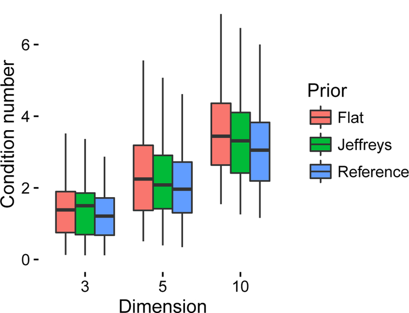
Median condition number by dimension and prior specification: box plots describe distributions of 100 median condition numbers for each dimension and prior. Each point is the median from 200 posterior samples based on independent data and using gLMC. The reference prior is designed to yield smaller condition numbers than Jeffreys prior and hence better asymptotics [21].

Again, these priors are not intended to form a comprehensive list but give an idea of the kinds of choices that statisticians might make when choosing a prior for a covariance. For more recent developments in this area, see [25] and [26].

7. Results

This section features empirical validation of the gLMC algorithm as well as an application to learning the spectral density matrix for vector time series. For empirical validation, we present quantile-quantile and trace plots comparing the gLMC sample to the closed-form solution made available by the conjugate prior. We then use gLMC for Hermitian PD matrices to learn the spectral density matrices of both simulated and LFP time series. We use the posteriors thus obtained to get credible intervals on the squared coherences for the vector time series.

7.1. Empirical validation

Before applying gLMC to spectral density estimation, we demonstrate validity by comparing samples from empirical posterior distributions of the Gaussian inverse-Wishart model obtained by gLMC and the closed-form solution. Note that our objective is to show that our proposed method provides valid results, similar to those obtained based on conjugate priors, while creating a flexible framework for eliciting and specifying prior distributions directly over the space of PD matrices. To this end, we compare element-wise distributions with quantile-quantile plots and whole-matrix distributions with two global matrix summaries. The comparisons based on 10,000 samples by the different sampling methods over 3-by-3 PD matrices are illustrated in Figure 2. The first 200 samples are discarded, and, for better visualization, every tenth sample is kept. For the global matrix summaries, we also include samples from an indirect approach, the log-Cholesky parameterization of the PD matrix (currently used in Stan software implementations [27]). Starting with a lower-triangular matrix L, one ob tains a PD matrix by exponentiating the diagonal elements of L to get $\tilde{L}$ and then evaluating $\sum =\tilde{L}{\tilde{L}}^T$. Given a distribution over PD matrices, one may obtain a distribution over lower-triangular matrices using the inverses of these transforms and their corresponding Jacobians.

Figure 2.

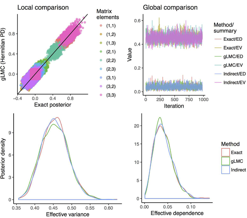
These figures provide empirical validation for the well-posedness of gLMC for PD matrices. On the top-left is a quantile-quantile plot comparing the gLMC (for Hermitian PD matrices) posterior sample with that of the closed-form posterior for the complex Gaussian inverse-Wishart model. Both real and imaginary elements are included, and points are jittered for visibility. On the top-right are posterior samples of ‘global’ matrix summaries pertaining both to gLMC (for symmetric PD matrices), the closed-form ‘exact’ solution, and the ‘indirect’ log-Cholesky parameterization. These summaries are the effective variance and the effective dependence, built off the covariance matrix and the correlation matrix, respectively. On the bottom are posterior density plots of the same matrix summaries.

On the top-left panel of Figure 2, a quantile-quantile (Q-Q) plot is used to compare the gLMC Hermitian PD posterior sample to the closed-form posterior. The Q-Q plot is the gold standard for comparing two scalar distributions using empirical samples because full quantile agreement corresponds to equality of cumulative distribution functions. Points are jittered for easy visualization, and each color specifies a different matrix element. Note that some colors appear twice: these double appearances correspond to real and imaginary matrix elements. For example, pink appears at zero as well as the upper right of the plot: this color corresponds to a diagonal matrix element since, on account of the matrix being Hermitian, its imaginary part is fixed at zero. Most importantly, all matrix elements fit tightly around the line y = x, suggesting a perfect match in quantiles between empirical distributions.

On the top-right panel of Figure 2, we present samples obtained from two wholematrix summaries using gLMC, the ‘exact’ closed-form posterior, and the ‘indirect’ log-Cholesky parameterization. These summaries are the effective variance (EV) and the effective dependence (ED):

$$\text{EV}(\sum )=|\sum {|}^{1/d},\hspace{1em}\text{and}\hspace{1em}\text{ED}(\sum )=1-|\text{corr}(\sum ){|}^{1/d}.$$ (35)

The EV is the geometric mean of the eigenvalues of the matrix Σ. It provides a dimension free summary of the total variance encoded in the matrix. The ED gets its name because the determinant of a correlation matrix is inversely related to the magnitude of the individual correlations that make up the off-diagonals. In addition to seeing that element-wise distributions match, one would also like to know that their joint distributions correspond. The EV and ED are good summaries of global matrix features and here provide empirical evidence for the validity of gLMC for PD matrices. As we can see, the three methods have similar posterior distributions of EV and ED (Figure 2, bottom panels).

7.2. Learning the spectral density

An important benefit of gLMC is that it enables practitioners to specify prior distributions other than the inverse-Wishart on PD matrices based on needs dictated by the problems at hand. gLMC improves modeling flexibility. We use the problem of Bayesian spectral density estimation to demonstrate the possibility and advantage of using non-conjugate priors. The spectral density matrix Σ(ω) and its coherence matrix R(ω) are defined in Section 2. In the context of stationary, multivariate time series, the coherences that make up the off-diagonals of R(ω) provide a lag-free measure of dependence between univariate time series at a given frequency ω. Hence, these coherences are among the more interpratable parameters of the spectral density matrix.

We compare posterior inference for these coherences between two models with different priors: the first model uses the complex inverse-Wishart prior; the second uses the complex reference prior [24]. The reference prior is an improper prior that has been proposed as an alternative to Jeffrey’s prior for its superior eigenvalue shrinkage (which improves asymptotic efficiency of estimators). We use the reference prior to emphasize the flexibility allowed by gLMC but not as a modeling suggestion. [24] provide a Gibbs sampling routine based on the eigen-decomposition of the covariance matrix. The reference prior’s form is provided in Appendix A.1.

We apply gLMC to learning the spectral density matrix for three distinct 4-dimensional time series. The first is a simulated first-order vector-autoregressive (VAR1) time series with block structure consisting of two independent, 2-dimensional VAR1 time series. The second time series is also VAR1 but with dependencies allowed between all four of the scalar time series of which it is composed. The third time series comes from local field potentials (LFP) recorded in the CA1 region of a rat hippocampus [28].

Figure 3 shows the first 100 samples from both VAR1 time series along with 95% posterior intervals for the complex moduli of the coherences. The time series are simulated with the form:

$$y\left(t\right)=\Phi y\left(t-1\right)+{ϵ}_t,\hspace{1em}\hspace{1em}y\left(1\right)={ϵ}_1,\hspace{1em}\hspace{1em}{ϵ}_t\sim {{\rm N}}_4\left(0,I\right),t=1,\mathrm{...},15000,$$ (36)

where the eigenvalues of transition matrix Φ are bounded with absolute value less than 1 to induce stationarity. The first 10,000 data points are discarded to allow time for mixing. The first row of Figure 3 belongs to the block VAR1: Φ is a randomly constructed, block-diagonal matrix, so the first two scalar time series are independent from the second two. The second row of Figure 3 belongs the the second VAR1, all the scalar time series of which are dependent on all the others. Here Φ is also a randomly constructed matrix but is not block-diagonal. The intervals corresponding to the inverse-Wishart prior model are given in orange. The intervals corresponding to the reference prior model are given in blue. The true coherences are represented by black points and are obtained using the following closed-form formula for the spectral density of a VAR1 process [10]:

$$\sum \left(\omega \right)={\left(I-\Phi e^{-2\pi i\omega }\right)}^{-1}Q{\left(I-\Phi e^{-2\pi i\omega }\right)}^{-H}.$$ (37)

Here Q is the covariance matrix of the additive noise ∈_t, and (·)^−H denotes the inverse conjugate transpose. For the block VAR1 example, both models capture the true, non-null coherences (i.e. those given on the far left and the far right), but neither captures the null coherences. This is more than satisfactory, since coherences equal to zero imply the identity for a covariance matrix. By looking closely, one can see that the first and second time series (orange and green) are indeed strongly dependent on each other, as interval ‘1:2’ suggests. For the full VAR1 example, both models capture five out of six true coherences, but the reference prior model gets closer to the truth than the inverse-Wishart model does.

Figure 3.

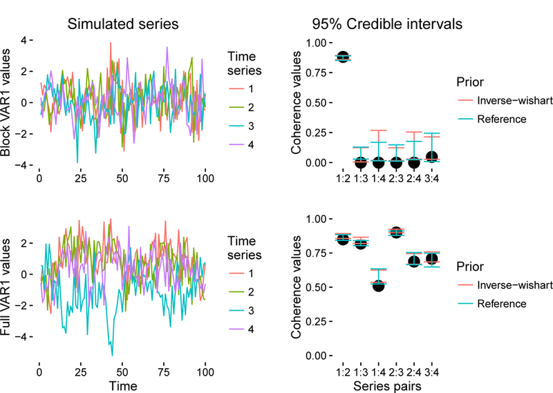
Two 4-dimensional VAR1 time series and credible intervals for their 6 corresponding coherences measured at 20–40 Hz: the top row belongs to a block VAR1 process characterized by two independent 2-dimensional VAR1 time series; the bottom row belongs to a full VAR1 process. The left column shows the first 100 samples of both time series, each of which totals 5,000 samples in length. The right column shows credible intervals from posteriors obtained using the inverse-Wishart and reference priors.

We use the same tools to detect coherences between LFP signals simultaneously recorded from the CA1 region of a rat hippocampus prior to a memory experiment [28]. Two of the LFP signals are recorded on one end of the CA1 axis, and the other two LFP signals are recorded at the opposite end. Figure 4 shows the first 200 of 4,000 samples (recorded at 1,000 Hz) and 95% credible intervals for the coherences at two different frequency bands: 20–40 Hz and 40–160 Hz. The spatial discrepancy is reflected in the posterior distributions of the individual coherences. Both bands show similar coherence patterns, where spatial location appears to dictate strength of coherence: the leftmost and rightmost pairs are closer to each other in space, while the center pairs are farther from each other. This reflects what is apparent in the top of Figure (4), where the first and second time series (orange and green) are dependent, and the third and fourth time series (blue and purple) are dependent. These correspond to the intervals labeled ‘1:2’ and ‘3:4’, respectively. The credible intervals are smaller for the 20–40 Hz band because that band has only 1/6 the data of the 40–160 Hz band. Between prior models, the intervals differ more for the 40–160 Hz band. This is counter-intuitive since the influence of the prior distribution is often assumed to diminish with the size of the data set. One question is whether this surprising result is related to the reference prior’s being the prior that is ‘maximally dominated by the data’ [29]. These differences—differences between posterior distributions for the two prior models—communicate that other prior distributions might provide tangible differences between results in spectral analysis and that it would be useful to understand which prior distributions are appropriate in which contexts.

Figure 4.

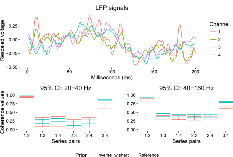
A 4-dimensional LFP signal with credible intervals for 6 coherences measured at 20–40 Hz (left) and 40–160 Hz (right). First 200 samples are shown for ease of visualization; the multi-dimensional time series totals 4,000 samples in length. Coherence profiles are remarkably similar between the two frequency bands considered.

8. Discussion

We presented geodesic Lagrangian Monte Carlo an MCMC methodology for Bayesian inference on general Riemannian manifolds. We outlined its relationship to other geometric extensions of HMC and showed how to apply gLMC to both symmetric and Hermitian PD matrices. We demonstrated empirical validity using both element-wise and whole-matrix comparisons against the conjugate inverse-Wishart model. Finally, we applied gLMC on Hermitian PD matrices to Bayesian spectral density estimation. The algorithm proved effective for detecting true coherences of simulated time series, as well as recovering spatial discrepancies between real-world LFP signals.

We see three branches of inquiry stemming from this work: the first is algorithmic; the second, theoretical; the third, methodological. First, what variations of HMC might help extend gLMC over PD matrices into higher dimensions? There are multiple such extensions that are orthogonal to gLMC. Examples are windowed HMC, geometric extensions to the NUTs algorithm, shortcut MCMC, and look-ahead HMC [5, 30, 31]. Auto-tuning will prove useful: even within the same dimension, different samples will dictate different numbers of leapfrog steps and step-sizes. From the theoretical standpoint, the canonical metric on the space of PD matrices is closely related to the Fisher information metric on covariance matrices: how should one characterize this intersection between information geometry and Riemannian symmetric spaces, and how might this relationship inform Bayes estimator properties or future variations on gLMC? Methodologically, much work needs to be done in prior elicitation for Bayesian spectral density estimation.Which priors on Hermitian PD matrices should be used for which problems, what are the costs and benefits, and are there priors over symmetric PD matrices that need to be complexified (cf. [25, 26])? A clear delineation will be useful for practitioners in Bayesian time series research.

Appendix A. Real and complex matrix derivatives

The derivative of a univariate, real valued function with respect to a matrix is most cleanly calculated using the matrix differential. This is true whether $f:M_p\left(ℝ\right)\mapsto ℝ$ or $f:M_p\left(ℂ\right)\mapsto ℝ,$ i.e. whether f is a function over real p × p matrices or complex p × p matrices. As an example, we consider the multivariate Gaussian distribution with mean 0 and covariance Σ. First, let f be the probability density function over real valued Gaussian random vectors $y_n\in {ℝ}^d,n=1,\mathrm{...},N$. Let Y be the d × N concatenation of these N i.i.d. random variables. Then the log density is given by

$$\begin{array}{l}\log f\left(Y^N,\sum \right)\propto -\frac{N}{2}\log |\sum |-\frac{1}{2}\sum _{n=1}^N{y}_n^T{\sum }^{-1}{y}_n\\ \hspace{1em}\hspace{1em}\hspace{1em}\hspace{1em}\hspace{1em}\hspace{0.17em}\hspace{0.17em}\hspace{0.17em}=-\frac{N}{2}\log |\sum |-\frac{1}{2}\text{tr}\left\{{\sum }^{-1}Y{Y}^T\right\}.\end{array}$$ (A1)

We apply the matrix differential to (A1) using two general formulas:

$$d\log |\sum |=\text{tr}\left\{{\sum }^{-1}d\sum \right\},\hspace{0.17em}\hspace{0.17em}\text{and}\hspace{0.17em}\hspace{0.17em}d{\sum }^{-\text{1}}=-{\sum }^{-1}\left(d\sum \right){\sum }^{-1},$$ (A2)

rendering

$$\begin{array}{l}d\log f\left(Y,\sum \right)=-\frac{N}{2}\text{tr}\left\{{\sum }^{-1}d\sum \right\}+\frac{1}{2}\text{tr}\left\{{\sum }^{-1}\left(d\sum \right){\sum }^{-1}Y{Y}^T\right\}\\ \hspace{1em}\hspace{1em}\hspace{1em}\hspace{1em}\hspace{1em}\hspace{0.17em}\hspace{0.17em}=-\frac{N}{2}\text{tr}\left\{\left(d\sum \right){\sum }^{-1}\right\}+\frac{1}{2}\text{tr}\left\{\left(d\sum \right){\sum }^{-1}Y{Y}^T{\sum }^{-1}\right\}.\end{array}$$ (A3)

Finally, we relate the matrix differential to the gradient with the fact that, for an arbitrary function g,

$$dg(\sum )=\text{tr}\left\{\left(d\sum \right)A\right\}\hspace{1em}\iff \hspace{1em}{\nabla }_{\sum }g(\sum )=A.$$ (A4)

This gives the final form of the gradient of the log density function with respect to covariance Σ:

$${\nabla }_{\sum }\log f\left(Y,\sum \right)=-\frac{N}{2}{\sum }^{-1}+\frac{1}{2}{\sum }^{-1}Y{Y}^T{\sum }^{-1}.$$ (A5)

For more on the matrix differential, see [32]. The complex matrix differential is treated in [33] and has a similar form real valued functions. The log density of the multivariate complex Gaussian with mean 0 is given by

$$\begin{array}{l}\log f\left(Y,\sum \right)\propto -N\log |\sum |-\sum _{n=1}^N{y}_n^H{\sum }^{-1}{y}_n\\ \hspace{1em}\hspace{1em}\hspace{1em}\hspace{1em}\hspace{1em}=-N\log |\sum |-\text{tr}\left\{{\sum }^{-1}Y{Y}^H\right\},\end{array}$$ (A6)

where (·)^H denotes the conjugate transpose. Note that the log density is scaled by a factor of two compared to the real case. The resulting gradient is

$${\nabla }_{\sum }\log f\left(Y,\sum \right)=-N{\sum }^{-1}+{\sum }^{-1}Y{Y}^H{\sum }^{-1}.$$ (A7)

A.1. The complex reference prior

Gradients of prior probabilities are calculated in a similar way. We demonstrate for the complex reference prior. Let ${\lambda }_i,i=1,\mathrm{...},d$ be the decreasing eigenvalues of Hermitian PD matrix Σ. Then the complex reference prior has the following form:

$$p(\sum )\propto \frac{\text{d}\sum }{|\sum |\prod {}_{k<j}{\left({\lambda }_k-{\lambda }_j\right)}^2}.$$ (A8)

To use the above approach for deriving the matrix derivatives, we need to be able to write the differential $d{\lambda }_i$ in terms of the matrix differential dΣ. [32] provides the formula when all eigenvalues are distinct:

$$d{\lambda }_i=\text{tr}\left(\sum _{j=1}^d{V}_{ij}^{-1}{\sum }^{j-1}d\sum \right),$$ (A9)

where V is the Vandermonde matrix:

$$V^{\text{T}}=\left|\begin{array}{cccccc}1& {\lambda }_{\text{1}}& {\lambda }_1^2& \cdots & {\lambda }_1^{n-2}& {\lambda }_1^{n-1}\\ 1& {\lambda }_{\text{2}}& {\lambda }_2^2& \cdots & {\lambda }_2^{n-2}& {\lambda }_2^{n-1}\\ ⋮& ⋮& ⋮& \ddots & ⋮& ⋮\\ 1& {\lambda }_n& {\lambda }_n^2& \cdots & {\lambda }_n^{n-2}& {\lambda }_n^{n-1}\end{array}\right|.$$ (A10)

We now calculate the gradient of the log of the complex reference prior:

$$\begin{array}{l}d\log p(\sum )=-d\log |\sum |-2\sum _{k<j}d\log \left({\lambda }_k-{\lambda }_j\right)\\ \hspace{0.17em}\hspace{1em}\hspace{1em}\hspace{1em}\hspace{1em} =-\text{tr}\left({\sum }^{-1}d\sum \right)-2\sum _{k<j}\frac{d{\lambda }_k-d{\lambda }_j}{{\lambda }_k-{\lambda }_j}\\ \hspace{0.17em}\hspace{1em}\hspace{1em}\hspace{1em}\hspace{1em} =-\text{tr}\left({\sum }^{-1}d\sum \right)-2\sum _{k<j}\text{tr}\left(\sum _{i=1}^d\left(V_{ki}^{-1}-V_{ji}^{-1}\right){\sum }^{i-1}d\sum \right)/\left({\lambda }_k-{\lambda }_j\right).\end{array}$$ (A11)

Combining this with Equations (A2) and (A4) renders matrix gradient

$${\nabla }_{\sum }\log p(\sum )\propto -{\sum }^{-1}-2\sum _{k<j}\left(\sum _{i=1}^d\left(V_{ki}^{-1}-V_{ji}^{-1}\right){\sum }^{i-1}\right)/\left({\lambda }_k-{\lambda }_j\right).$$ (A12)

References

- [1].Tokuda T, Goodrich B, Van Mechelen I, et al. Visualizing distributions of covariance matrices. Dept Statist, Columbia Univ, New York, NY, USA, Tech Rep. 2011;. [Google Scholar]
- [2].Girolami M, Calderhead B. Riemann manifold langevin and hamiltonian monte carlo methods. Journal of the Royal Statistical Society: Series B (Statistical Methodology) 2011;73(2):123–214. [Google Scholar]
- [3].Byrne S, Girolami M. Geodesic monte carlo on embedded manifolds. Scandinavian Journal of Statistics 2013;40(4):825–845. [DOI] [PMC free article] [PubMed] [Google Scholar]
- [4].Lan S, Zhou B, Shahbaba B. Spherical hamiltonian monte carlo for constrained target distributions. In: JMLR workshop and conference proceedings; Vol. 32; NIH Public Access; 2014. p. 629. [PMC free article] [PubMed] [Google Scholar]
- [5].Neal RM, et al. Mcmc using hamiltonian dynamics. Handbook of Markov Chain Monte Carlo 2011;2:113–162. [Google Scholar]
- [6].Lan S, Stathopoulos V, Shahbaba B, et al. Markov chain monte carlo from lagrangian dynamics. Journal of Computational and Graphical Statistics 2015;24(2):357–378. [DOI] [PMC free article] [PubMed] [Google Scholar]
- [7].Shahbaba B, Lan S, Johnson WO, et al. Split hamiltonian monte carlo. Statistics and Computing 2014;24(3):339–349. [Google Scholar]
- [8].Pourahmadi M Covariance estimation: The glm and regularization perspectives. Statistical Science 2011;:369–387.
- [9].Abramovich YI, Besson O. On the expected likelihood approach for assessment of regularization covariance matrix. IEEE Signal Processing Letters 2015;22(6):777–781. [Google Scholar]
- [10].Wang YHL, H O. Statistical analysis of electroencephalograms CRC Press; 2016. p. 523–565. [Google Scholar]
- [11].Whittle P The analysis of multiple stationary time series. Journal of the Royal Statistical Society Series B (Methodological) 1953;:125–139.
- [12].Brockwell PJ, Davis RA. Time series: theory and methods Springer Science & Business Media; 2013. [Google Scholar]
- [13].Gao X, Shahbaba B, Fortin N, et al. Evolutionary state-space model and its application to time-frequency analysis of local field potentials arXiv preprint arXiv:161007271. 2016;. [DOI] [PMC free article] [PubMed]
- [14].Pennec X, Fillard P, Ayache N. A riemannian framework for tensor computing. International Journal of Computer Vision 2006;66(1):41–66. [Google Scholar]
- [15].Moakher M, Zéraϊ M. The riemannian geometry of the space of positive-definite matrices and its application to the regularization of positive-definite matrix-valued data. Journal of Mathematical Imaging and Vision 2011;40(2):171–187. [Google Scholar]
- [16].Helgason S Differential geometry, lie groups, and symmetric spaces Vol. 80 Academic press; 1979. [Google Scholar]
- [17].Koh SS. On affine symmetric spaces. Transactions of the American Mathematical Society 1965;119(2):291–309. [Google Scholar]
- [18].Duane S, Kennedy AD, Pendleton BJ, et al. Hybrid monte carlo. Physics letters B 1987; 195(2):216–222. [Google Scholar]
- [19].Nash J The imbedding problem for riemannian manifolds. Annals of mathematics 1956; :20–63.
- [20].Lan S, Shahbaba B. Sampling constrained probability distributions using spherical augmentation Cham: Springer International Publishing; 2016. p. 25–71. [Google Scholar]
- [21].Yang R, Berger JO. Estimation of a covariance matrix using the reference prior. The Annals of Statistics 1994;:1195–1211.
- [22].Shaman P The inverted complex wishart distribution and its application to spectral estimation. Journal of Multivariate Analysis 1980;10(1):51–59. [Google Scholar]
- [23].Svensson L, Lundberg M. On posterior distributions for signals in gaussian noise with unknown covariance matrix. IEEE Transactions on Signal Processing 2005;53(9):3554–3571. [Google Scholar]
- [24].Svensson L, Nordenvaad ML. The reference prior for complex covariance matrices with efficient implementation strategies. IEEE Transactions on Signal Processing 2010;58(1):53–66. [Google Scholar]
- [25].Schwartzman A Lognormal distributions and geometric averages of symmetric positive definite matrices. International Statistical Review 2015;. [DOI] [PMC free article] [PubMed]
- [26].Fazayeli F, Banerjee A. The matrix generalized inverse gaussian distribution: Properties and applications arXiv preprint arXiv:160403463. 2016;.
- [27].Carpenter B, Gelman A, Hoffman M, et al. Stan: A probabilistic programming language. Journal of Statistical Software 2016;20:1–37. [DOI] [PMC free article] [PubMed] [Google Scholar]
- [28].Allen TA, Salz DM, McKenzie S, et al. Nonspatial sequence coding in ca1 neurons. The Journal of Neuroscience 2016;36(5):1547–1563. [DOI] [PMC free article] [PubMed] [Google Scholar]
- [29].Berger JO, Bernardo JM, Sun D. The formal definition of reference priors. The Annals of Statistics 2009;:905–938.
- [30].Sohl-Dickstein J, Mudigonda M, DeWeese MR. Hamiltonian monte carlo without detailed balance arXiv preprint arXiv:14095191. 2014;.
- [31].Betancourt M Generalizing the no-u-turn sampler to riemannian manifolds arXiv preprint arXiv:13041920. 2013;.
- [32].Magnus JR, Neudecker H, et al. Matrix differential calculus with applications in statistics and econometrics 1995;.
- [33].Hjorungnes A, Gesbert D. Complex-valued matrix differentiation: Techniques and key results. IEEE Transactions on Signal Processing 2007;55 (6): 2740–2746. [Google Scholar]