

Abstract
Exposure to environmental mixtures can exert wide-ranging effects on child neurodevelopment. However, there is a lack of statistical methods that can accommodate the complex exposure-response relationship between mixtures and neurodevelopment while simultaneously estimating neurodevelopmental trajectories. We introduce Bayesian varying coefficient kernel machine regression (BVCKMR), a hierarchical model that estimates how mixture exposures at a given time point are associated with health outcome trajectories. The BVCKMR flexibly captures the exposure-response relationship, incorporates prior knowledge, and accounts for potentially nonlinear and nonadditive effects of individual exposures. This model assesses the directionality and relative importance of a mixture component on health outcome trajectories and predicts health effects for unobserved exposure profiles. Using contour plots and cross-sectional plots, BVCKMR also provides information about interactions between complex mixture components. The BVCKMR is applied to a subset of data from PROGRESS, a prospective birth cohort study in Mexico city on exposure to metal mixtures and temporal changes in neurodevelopment. The mixture include metals such as manganese, arsenic, cobalt, chromium, cesium, copper, lead, cadmium, and antimony. Results from a subset of Programming Research in Obesity, Growth, Environment and Social Stressors data provide evidence of significant positive associations between second trimester exposure to copper and Bayley Scales of Infant and Toddler Development cognition score at 24 months, and cognitive trajectories across 6–24 months. We also detect an interaction effect between second trimester copper and lead exposures for cognition at 24 months. In summary, BVCKMR provides a framework for estimating neurodevelopmental trajectories associated with exposure to complex mixtures.
Keywords: Bayesian inference, chemical mixtures, child health, longitudinal data, machine learning, neurodevelopment
1 |. INTRODUCTION
Environmental exposures can exert wide-ranging effects on children’s neurodevelopment and cognition. While the literature tends to focus on the effects of exposure to a single chemical, in reality, we are exposed to complex chemical mixtures through diet and pollution in daily life. Environmental mixtures are a priority area of the National Institute of Environmental Health Sciences, which has placed an emphasis on elucidating their associated health effects.1 Many environmental exposures can be thought of as complex mixtures. For example, air pollution can be viewed as a mixture of ozone, particulate matter, volatile organic compounds, and other particulates. Metal mixtures are another type of complex mixture, comprising of metals such as lead, arsenic, manganese, and zinc. Numerous articles have reported on the neurodevelopmental effects of perinatal exposure to chemicals, such as pesticides, heavy metals, insecticides, lead, and methyl mercury,2–6 but few have addressed how complex chemical mixtures affect the longitudinal trajectory of development that is a hallmark of childhood. This paper will present a modeling framework by which mixtures can be used to predict time varying changes in child development.
In this article, we investigate how exposure to metal mixtures in early life impacts neurodevelopmental trajectories. During fetal life and early childhood, neurodevelopmental processes are rapid, sequential, and specifically timed, such that exposure to toxicants in fetal life can cause lifelong effects that may begin as incremental changes in health.7 Many metals cross the placental barrier and could potentially harm the fetal brain.8,9 Heavy metal mixture exposures may delay the development of the central nervous system; even weak signals could alter a normal cognitive trajectory to a maladaptive one. However, the literature on the health effects of metal mixtures is sparse, when compared to the established literature on the health effects of single metals. For example, while the effect of lead on child neurodevelopment has been well researched, exposure to metal mixtures rather than to individual metals is more reflective of real-world exposure.
There are several challenges to modeling the longitudinal effects of exposure to metal mixtures. Some of these challenges are ubiquitous to analyses of mixtures, whether in a cross-sectional or longitudinal setting. They include (i) high correlation among the mixture components, leading to potential challenges in disentangling the particular effects of a specific mixture component; and (ii) potential interactive (eg, synergistic or antagonistic) relationships among mixture components. Detectable mixture effects on health may still exist when individual metal exposures are below no observable adverse effect levels.10 Researchers have also found evidence of interactions between metals. Summarizing the literature on metal mixture effects, Claus Henn et al11 reported increased lead toxicity in the presence of higher levels of manganese, arsenic, and cadmium for outcomes such as cognition, neurodevelopment, and reproductive hormone levels. (iii) The exposure-response relationship between metal mixture exposures and neurodevelopment may be complex, exhibiting both nonlinearity and nonadditivity. For example, manganese has dual roles, ie, it functions as an essential nutrient at low doses but as a neurotoxicant at high doses, resulting in an inverted-u relationship with neurodevelopment.12 These challenges of estimating mixture effects while accounting for potential interaction, high correlation among mixture components, and potentially nonlinear and nonadditive mixture effects, are further exacerbated in a longitudinal setting. When we estimate the longitudinal health effects associated with exposure to mixtures at a single time window, it is important to account for potential correlation from repeated measures of the outcome within an individual. Furthermore, the mixture may exert effects on different features on the longitudinal trajectory; for example, it could have effects on the level of the outcomes or the rate of change in the longitudinal outcomes. This necessitates models that can flexibly account for characteristics of mixtures, along with model parameters that are associated with longitudinal measures of health outcomes.
There is a lack of existing statistical models that can flexibly capture the longitudinal impact of exposure to chemical mixtures. A workshop13 held in 2015 by the National Institute of Environmental Health Sciences compared 30 statistical approaches for mixtures, which broadly fall within the categories of classification and prediction, exposure-response surface estimation, variable selection, and variable shrinkage strategies. Two kernel-learning approaches for exposure-response surface estimation, called Bayesian kernel machine regression14 for estimation of mixtures at a single time window and lagged kernel machine regression15,16 for estimation of time-varying mixtures, can model potentially complex exposure-response relationships. These methods allow researchers to predict health effects for unobserved exposure profiles and visualize interactions between components of the mixture. However, these methods, like many methods for mixtures, are generally designed for outcomes measured at a single time point. Unfortunately, there are limited strategies to handle estimation of exposure mixture effects in longitudinal outcome settings. While mixed effect models can handle the correlation of repeated outcomes data, they may not perform well in situations of highly correlated exposure data, such as in the case of chemical mixtures. One potential work-around is to embed techniques for modeling mixtures, such as kernels,14–16 weighted quantile sum regression,17 principal components analysis, environmental risk score,18 among other approaches, within a mixed model for longitudinal data.
In this article, we seek to develop a method that can both characterize the exposure-response surface, such as visualize the interaction between mixture components for new, unobserved exposure profiles, as well as assess the directionality and relative importance of a metal on health outcome trajectories. This can help identify the components of the mixture that are drivers of the longitudinal health effects, and these components could be targeted for public health intervention. Thus, we propose a new Bayesian hierarchical model, termed Bayesian varying coefficient kernel machine regression (BVCKMR). This is a flexible method, meaning that it can allow for the investigation of complex exposure-response relationships and can account for the possibility of nonlinear and nonadditive effects of individual exposures. We will model the exposure-response surface at baseline cognition and for cognitive trajectories and predict how the exposure-response surface changes at new exposure mixture profiles. Furthermore, we seek to estimate changes in interaction and effect modification between mixtures of heavy metals over time. Lastly, the Bayesian modeling approach allows us to potentially incorporate prior knowledge from previous studies or subject matter experts. Our method provides a conceptual framework for the estimation of neurodevelopmental trajectories associated with exposure to metal mixtures.
We apply the BVCKMR model to data from the ongoing Programming Research in Obesity, Growth, Environment and Social Stressors (PROGRESS) study. PROGRESS is an NIH-funded, prospective prebirth cohort study followed in Mexico city. Exposure to multiple metals has been measured, including manganese (Mn), lead (Pb), cobalt (Co), chromium (Cr), cesium (Cs), copper (Cu), arsenic (As), cadmium (Cd), and antimony (Sb) from maternal blood at the second trimester of pregnancy. Our neurodevelopmental outcomes of interest are Bayley Scales of Infant and Toddler Development, Third Edition (BSID-III) scores assessed at 6, 12, 18, and 24 months after birth. In our data application, we estimate the neurodevelopmental trajectories associated with joint exposures during the second trimester of pregnancy to nine metals (Mn, Pb, Co, Cr, Cs, Cu, As, Cd, and Sb).
The objective of this article is to introduce the BVCKMR model to researchers in epidemiology and biostatistics and illustrate its use in estimating neurodevelopmental trajectories associated with exposure to heavy metal mixtures. The paper is organized as follows. In Section 2, we provide a brief review of Bayesian KMR. In Section 3, we introduce the statistical model BVCKMR. In Section 4, we describe the simulation studies for evaluating performance of BVCKMR, and in Section 5, we apply the method to data from the PROGRESS cohort study. Finally, in Section 6, we provide discussion and concluding remarks in the context of the environmental health literature.
2 |. REVIEW OF BAYESIAN KERNEL MACHINE REGRESSION
We review the kernel machine regression (KMR) framework, which can be used to estimate the impact of exposure to a complex mixture, when both outcome and exposures are measured at a single time point. Bayesian KMR has been used to flexibly model the relationship between complex mixtures and a health outcome, and the estimated parameters can be used to predict health effects of unobserved exposure mixtures.14 Suppose we observe data from n subjects with continuous, normally distributed outcomes. For each subject i = 1, … , n, the outcome (yi) is related to M components of the exposure mixture zi = (z1i, … , zMi)T through a parametric or nonparametric function, ie, h(·), while controlling for p relevant confounders xi = (x1i, … , xpi)T. The model is
| (1) |
β represents the effects of the potential confounders, and . We use a kernel representation for h (·), the unknown function, as the exposure-response relationship may be complex.
There are choices for specifying h (·). We can specify it either through basis functions or through a positive definite kernel function K (·, ·). The kernel function K (·, ·) implicity specifics a unique function space, ie, Hk, that is spanned by a set of orthogonal basis functions, according to Mercer’s theorem.20 A function h (·) ∈ Hk can be specified through a set of basis functions under the primal representation or through a kernel function under the dual representation. Under the dual representation, K(·, ·) can be thought of as a metric that quantifies the similarity between exposure profiles zi and zj for any two subjects i and j in the study. By choosing different kernel functions, we can control the complexity and form of the exposure-response function.
Kernel methods are used in broad applications in public health, such as statistical genetics and environmental health. Depending on the data application, many types of kernel choices are possible (see review by Wang et al21). Kernel choices that have been used in the environmental health literature include (i) the Gaussian kernel,14 which quantifies the distance or similiarity between two individual’s exposures using the Euclidean distance; and (ii) the polynomial kernel,15 which quantifies the dstiance between two individual’s exposures using the inner product, with the form .
Previous literature has also connected kernel machine methods with linear mixed models,22 showing that (1) can be expressed as the mixed model
| (2) |
| (3) |
where hi represents the subject-specific exposure-response effect, K is a kernel matrix with i, jth element K(zi, zj), and GP stands for Gaussian Process.
3 |. BAYESIAN VARYING COEFFICIENT KERNEL MACHINE REGRESSION MODEL FORMULATION
Now, suppose that exposures to a complex mixture are measured at a single time point, but we have repeated measures on the outcome, with the goal of identifying the longitudinal health impact of exposure and predicting health effects of new exposure mixtures. We consider a random effects model in which each subject i = 1, … , n has outcomes measured at ages j = 1, … , Ji, where Ji may differ depending on the subject i. We relate the outcome (yij) to M components of the exposure mixture zi = (z1i, …, zMi)T through two flexible functions, ie, h1(·) and h2(·). We again control for p relevant confounders xi = (x1i, … , xpi). The BVCKMR model is defined as follows:
| (4) |
where hq (·), q = 1, 2 can be estimated parametrically or nonparametrically and represents the exposure-response functions for the exposures zi. ageij represents the age of the ith individual at the jth time point. h1 represents the cross-sectional relationship of the mixture components with the outcome at the baseline age (either age 0 or the mean age if ageij is centered), and h2 represents the association between the mixture components and the outcome trajectory over time. We allow for the potential existence of a global trend line, ie, γ1 + γ2 ∗ ageij, so that individual-level intercepts and slopes can be shrunk toward this line.
For simplicity, we write the random effects model as
| (5) |
for i = 1, … , n and repeated measures j = 1, … , Ji, and bi ∼ N2(0, σ2D) and , where the parameters are represented later. h is the vector of individual-specific effects. For individual i, h1,i corresponds to the individual-specific baseline outcome level, whereas h2,i corresponds to the individual-specific age-related trajectory of the health outcome. We again employ a kernel representation for hq (·) to accommodate the possibly complex exposure-response relationships. bi represents the random effects for subject i, where b1,i corresponds to the intercept and b2,i corresponds to the slope. Xi is a matrix of potential confounders for subject i, and β represents the effects of the potential confounders. The U and W matrices correspondingly represent the ages of different individuals. Yi is the vector of continuous outcomes for subject i, where . D is a q × q positive definite covariance matrix, and is an Ji × Ji identity matrix
Following a Bayesian parameterization of this random effects model, we can express 5 as a hierarchical model, where K denotes the kernel matrix with i,j element K(zi, zj). Depending on a particular application, a number of different kernel functions may be employed. The diagonal blocks of size n × n in Σh arise due to the kernel structure placed on each hq(·), q = 1, 2. The parameters γ1 and γ2 corresponding to the global trend line can be estimated by including an intercept and an age term in the X design matrix and estimating β. The hierarchical model is
| (6) |
| (7) |
| (8) |
Here, , are latent parameters corresponding to a Bayesian group lasso,23 which is designed to select groups of variables for prediction. In our case, the Bayesian group lasso corresponds to the complex mixture, with being a latent parameter for the effect of the mixture on the baseline health outcome and being a latent parameter for the effect of the mixture on the age-related health outcome trajectory. Following the parameterization of Kyung et al,23 we use the priors
| (9) |
and
| (10) |
A common prior distribution for the covariance matrix D is the Wishart; thus, we use the prior
| (11) |
Lastly, we set the priors for σ2 and β, where
| (12) |
and
| (13) |
3.1 |. Markov chain Monte Carlo sampler
We used a Gibbs sampler to implement BVCKMR, as detailed in the Supporting Information. We obtained R samples of (β(r), b(r), τ2(r), h(r), D−1(r), σ2(r), λ2(r)), r = 1, … , R. These draws constitute samples from the joint posterior distribution of (β, b, τ2, h, D−1, σ2, λ2|y).
3.2 |. Prediction of baseline cognition and cognitive trajectories at new exposure profiles
It is often of interest to estimate the exposure-response surface and predict health effects for new, unobserved exposure profiles. For example, we may be interesting in predicting the effect of a change in levels of exposure to a single metal while holding all other metals at their median exposure levels. The flexibility of the BVCKMR model allows for the prediction of the baseline and trajectory of the exposure-response function for g new metal mixture exposures. Using BVCKMR, we initially fit the model to data from n subjects, and then we seek to predict the exposure-response surfaces hq(·), q = 1, 2 at these g new mixture values, ie, , where . Our interest is in the newly predicted random effects for q = 1, 2 corresponding to the baseline and trajectory of the outcome, respectively. These random effects are estimated for new, unobserved subjects, with exposure profiles given the observed data.
In order to simplify derivations of the posterior distributions of the given the observed hq, we define as a reordered h vector, such that . The corresponding covariance matrix is reordered, and we denote this reordered matrix as . The joint distribution of observed and new exposure profiles is
| (14) |
where denotes the 2n × 2n matrix with (i, j)th element K(zi, zj), denotes the n × g matrix with (i, j)th element involving the observed mixture zi and a new mixture , and denotes the g × g matrix with (i, j)th element constructed using the kernel function evaluated at the new mixture exposure profiles.
The conditional posterior distribution of hnew is
| (15) |
It can be computationally burdensome to estimate hnew, as it requires simulation from a high-dimensional multivariate normal distribution. Here, we approximate the posterior mean and variance of hnew using their conditional posterior evaluated at the posterior mean of the other parameters.
4 |. SIMULATION STUDY
We conducted a simulation study to evaluate the performance of the proposed BVCKMR model for estimating hq, q = 1, 2. Our simulation study considered four scenarios in which different combinations of five toxicants exert an exposure-response effect. We chose K to be a quadratic kernel, such that K(z, z′) = (zTz′ + 1)2. We used the following model: , where εij ∼ N(0, 1), xi = (x1i, x2i), and x1i ∼ N (0, 1) and x2i ∼ Bernoulli(0.5). We simulated correlation between M = 5 toxicants based on existing data from the application study on metal mixture exposures. The forms of the simulated exposure-response functions hq(zm), q = 1, 2, were selected based on findings from the literature, which provide evidence of potentially quadratic relationships between metal mixtures and neurodevelopment. We simulated the exposure-response functions as (i) Linear, additive: h1(z) = 0.5 ∗ z1 and h2(z) = 0.5 ∗ z1; (ii) Linear with interaction terms: h1(z) = 0.5 * (0.5z1z2 + z1 + z2) and h2(z) = 0.5 ∗ (z1 − z2); (iii) Quadratic with interaction terms where two toxicants exert an effect: and ; and (iv) Quadratic with interaction where all five toxicants exert an effect: and . In conducting the analysis, both exposure covariates and confounder variables were centered about their means and scaled by their standard deviations. For all the simulation scenarios, we simulated data based on the assumption that the global trend line equals zero (γ1 = γ2 = 0) and present results corresponding to that assumption.
Table 1 presents the results of this simulation. For each simulated data set of n = 100, we assessed the performance by regressing the predicted on h, for h1 and h2. We present the intercept, slope, and R2 of the regressions over 100 simulations. Good estimation performance occurs when the intercept is close to zero, and the slope and R2 are both close to one. We also present the root mean squared error (RMSE). We see that the performance is consistent across all four simulation scenarios; for all scenarios and h1 or h2, the intercept ranges from −0.01 to 0, and the slope ranges from 0.99–1.02. The R2 ranges from 0.74–0.98 and is higher in simulation scenarios (3) and (4), which contain a true quadratic effect. Lastly, the RMSE is higher for h1 than for h2; across all scenarios, it is 0.31 for h1 and 0.17 for h2. This similarity is likely due to similar signal-to-noise ratios being used for all scenarios.
TABLE 1.
Simulation results, regression of on h
| Scenario | h Function | Intercept | Slope | R2 | RMSE |
|---|---|---|---|---|---|
| Linear, additive | 1 | 0 | 1.01 | 0.74 | 0.31 |
| 2 | 0 | 1.02 | 0.90 | 0.17 | |
| Linear, interaction | 1 | 0 | 1.01 | 0.88 | 0.31 |
| 2 | 0 | 1.01 | 0.93 | 0.17 | |
| Quadratic, interaction | 1 | 0 | 1.00 | 0.95 | 0.31 |
| 2 | 0 | 1.00 | 0.97 | 0.17 | |
| Quadratic, interaction, all toxicants | 1 | 0 | 0.99 | 0.96 | 0.31 |
| 2 | −0.01 | 1.00 | 0.98 | 0.17 |
Performance of estimated hq (z) across 100 simulated datasets, each with N = 100. Root mean squared error (RMSE) denotes the root mean squared error of the as compared to h. For the four simulation scenarios, the exposure-response functions hq (z), q = 1, 2, were simulated as (1) Linear, additive: h1(z) = 0.5 ∗ z1 and h2(z) = 0.5 ∗ z1; (2) Linear with interaction terms: h1(z) = 0.5 * (0.5z1z2 + z1 + z2) and h2(z) = 0.5 ∗ (z1 − z2); (3) Quadratic with interaction terms where two toxicants exert an effect: and ; and (4) Quadratic with interaction where all five toxicants exert an effect: and .
Because an important aspect of environmental health research is identifying the components of the mixtures that are most associated with health outcomes, we defined a measure called relative importance to quantify the impact of each component on both the baseline health outcome and the outcome trajectory. Each component’s relative importance is based on predicting the baseline outcome (h1) and outcome trajectory (h2) exposure-response functions at two new exposure profiles, one where that component is at high exposure (75th percentile) and another where that component is at low exposure (25th percentile). For example, if we are interested in estimating z1’s relative importance, we would predict the exposure-response functions h1 and h2 for high z1 and low z1 while holding other components of the mixture at their median exposure to isolate the effect of z1. The difference in the estimated h1 for high versus low z1 corresponds to the relative importance of component z1 on the baseline outcome. Similarly, the difference in the estimated h2 for high versus low z1 corresponds to the relative importance of component z1 on the outcome trajectory.
The simulation results are further illustrated in Figure 1, in which we plot the BVCKMR predicted versus true relative importance for each simulation scenario. The results for each simulation scenario were averaged across 100 datasets. For each dataset, the relative importance was estimated at the same set of exposure values, which generally correspond to the 75th versus 25th percentile of exposure, whereas the true known relative importance remains the same across datasets. The 95% interval for relative importance is defined as the predicted relative importance +∕− 1.96 times the square root of the predicted corresponding variance. For each scenario, the BVCKMR predicted mean relative importance and 95% interval are shown for each metal, while the true known relative importance is depicted by a red point. We see that the 95% intervals capture the true exposure-response effect for all scenarios, showing that h is predicted well for new mixture exposure profiles. Furthermore, Figure 2 shows the BVCKMR predicted versus true exposure-response surface for a grid of z1 and z2 values, at fixed values of z3, z4, z5. For each simulation study, the upper panel contains predicted estimates of h(z1, z2) using BVCKMR, while the lower panel contains the known true exposure-response surface for the same grid of points. The predicted exposure response surface was averaged across 100 datasets, each with the same grid of points. In order to avoid extrapolation, the heatmap only colored for grid points within a specified distance from the simulated observed data points. As the upper and lower panels match well, we again see that h is predicted well for new mixture exposure profiles.
FIGURE 1.

Comparison of the Bayesian varying coefficient kernel machine regression (BVCKMR) predicted versus the true relative importance for a simulation study. Four simulation scenarios were considered: A, linear, additive (top left); B, linear, interaction (top right); C, quadratic with interaction (bottom left); and D, quadratic with interaction with all toxicants exerting an effect (bottom right). Relative importance is quantified by the difference in the estimated main effect of a single metal at high exposure and low exposure, holding all other metals constant at median exposures. The simulation study for each simulation scenario was averaged across 100 datasets. For each dataset, the relative importance was estimated at the same set of exposure values, which generally correspond to the 75th versus 25th percentile of exposure, and the 95% interval for relative importance is defined as the predicted relative importance +/−1.96 times the square root of the predicted corresponding variance. For each scenario, the true know relative importance remains the same across datasets. For each scenario, the BVCKMR predicted mean relative importance and 95% interval are shown for each metal, whereas the true known relative importance is depicted by a red point [Colour figure can be viewed at wileyonlinelibrary.com]
FIGURE 2.

Comparison of the Bayesian varying coefficient kernel machine regression (BVCKMR) predicted versus the true exposure-response surfaces for a simulation study. Four simulation scenarios were considered: A, linear, additive (top left); B, linear, interaction (top right); C, quadratic with interaction (bottom left); and D, quadratic with interaction with all toxicants exerting an effect (bottom right). Plot of the posterior mean of the exposure-response surface for a fixed grid of z1 and z2, at fixed values of z3, z4, z5. For each simulation study, the upper panel contains predicted estimates of h(z1, z2) using BVCKMR, whereas the lower panel contains the known true exposure-response relationship for the same grid of points. The predicted exposure response surface was averaged across 100 datasets, each with the same grid of points. In order to avoid extrapolation, the heatmap only colored for grid points within a specified distance from the simulated observed data points [Colour figure can be viewed at wileyonlinelibrary.com]
5 |. APPLICATION
We applied BVCKMR to investigate the association between exposure to metal mixtures at the second trimester of pregnancy and early life cognitive trajectories. We used a subset (n = 665) of the PROGRESS study. Exposures to a panel of nine metals (arsenic, cadmium, cobalt, chromium, cesium, copper, manganese, lead, and antimony) at the second trimester of pregnancy were studied. Correlations among the metal exposures ranged from 0.05 to 0.41. Confounder variables included socioeconomic status (three categories, ie, low, middle, and high), mother’s hemoglobin during the second trimester of pregnancy, mother’s educational level (< high school, high school, > high school), child gender, mother’s WASI IQ, and Fenton’s birthweight z-scores. The longitudinal neurodevelopmental outcome variables were BSID-III composite cognition scores measured at four time points after birth, generally corresponding to 6, 12, 18, and 24 months of age. BSID-III scores are normed at 100 with a standard deviation of 15. For ease of analysis, we centered and scaled the BSID-III scores and present the z-scores in our subsequent analysis. In conducting the analysis, metal exposure levels were log-transformed, then centered and scaled. Confounder variables were centered and scaled, and outcome variables were also scaled. For ease of interpreting results, the time variable was coded such that ageij = (daysij − 730.485)/365.2425, where daysij indicates the number of days after birth at which a Bayley Scale test was administered for subject i, at the jth index of the repeated measure. This allows us to identify the effects of the metals on cognition at 24 months and on cognitive trajectories across 6–24 months of age. Because previous literature suggests an inverted-u exposure-response relationship between metal mixture exposures and neurodevelopment, we chose K to be a quadratic kernel. The Markov chain Monte Carlo (MCMC) sampler was run for 10 000 iterations, with 5000 used as burn-in. Geweke’s diagnostic24 was used to evaluate convergence and was implemented using the R package “coda.”25 Using this diagnostic, we compared the means of the earlier and later parts of the Markov chain (the first 10% and the last 50%) and found no evidence of lack of convergence. The z-statistics for all parameters were within the 95% confidence interval, indicating that the means are similar and the chain is stationary. We also calculated the effective sample size of the multivariate Markov chain using the R package “mcmcse,”26,27 which was found to be 1795. Further details about the MCMC sampler can be found in the Supporting Information.
As a preliminary analysis and as a comparison to the BVCKMR model, we fit all the metal exposure data simultaneously using a linear mixed effects model with random intercept and random slope in the R package “lme4.”28 We sought to identify the association between the second trimester metal mixture exposures and 24-month neurodevelopment (as measured by BSID-III cognition scores) as well as neurodevelopmental trajectories across 6–24 months while accounting for the confounder variables. The results are presented in Figure 3. Although no metals were identified as significant at the p = 0.05 level, there were several metals with p-values below p = 0.15, suggesting their effects could be further studied. At 24 months, copper was positively associated with neurodevelopment (p = 0.09), as was chromium (p = 0.09). Across 6–24 months, copper was positively associated with neurodevelopmental trajectories (p = 0.13), as was chromium (p = 0.10). In addition across 6–24 months, lead was negatively associated with the neurodevelopmental trajectories (p = 0.11), as was antimony (p = 0.11). Lastly, we detected a significant negative interaction between copper and lead with 24-month neurodevelopment (p = 0.03).
FIGURE 3.
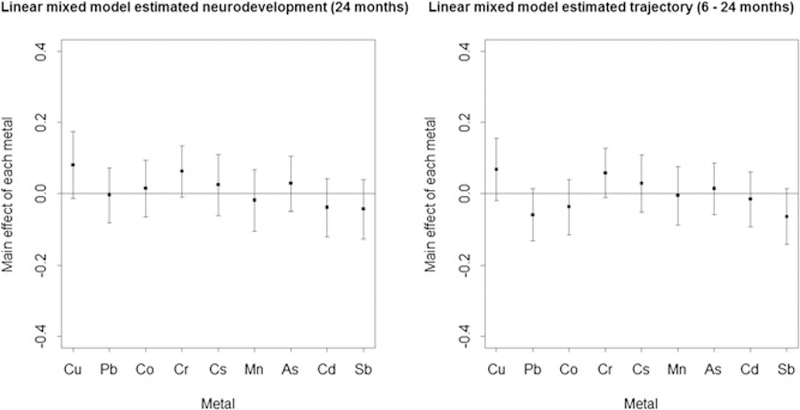
Linear mixed model estimated cognition at 24 months and cognitive trajectory (6–24 months) main effects applied to Programming Research in Obesity, Growth, Environment and Social Stressors data, accounting for random intercept and random slope. Plot of the main effects and 95% confidence intervals of Cu, Pb, Co, Cr, Cs, Mn, As, Cd, and Sb
We next use the BVCKMR model to fit the data. The posterior mean of the parameters related to the global trend line was γ1 = 0.50 and γ2 = −0.62, which correspond to the individual-level fixed effects of the intercept and slope. The magnitude of the posterior mean of and relative to σ2 provides an indication of how the total variability in the data decomposes into a complex mixtures component relative to an independent/excess varability component. In our data, we found that the posterior mean of σ2 was 0.36, whereas the posterior mean of both and was 2.65. The application results indicate that most of the variability lies in the complex mixtures, thus motivating the need to account for the mixtures effect in this model. Furthermore, we assessed the model fit of BVCKMR, using the deviance information criterion (DIC).29 The DIC is a measure of model fit, with smaller values indicating a better fit. We found that the BVCKMR model better fit the data (DIC = 4843.76) as compared with a Bayesian implementation of the comparable linear mixed model using the R package “MCMCglmm”30 (DIC = 5652.19). Using the BVCKMR model, we first estimated the relative importance of each metal for both neurodevelopment at 24 months and neurodevelopmental trajectories from 6–24 months, as shown in Figure 4. Relative importance is quantified by the difference in the estimated main effect of a single metal at high exposure (75th percentile) and low exposure (25th percentile), holding all other metals constant at median exposures. At 24 months, copper and chromium were significantly positively associated with neurodevelopment, whereas cadmium and antimony were significantly negatively associated with neurodevelopment. Across 6–24 months, copper and chromium were significantly positively associated with neurodevelopmental trajectories, whereas lead and antimony were significantly negatively associated with neurodevelopmental trajectories. Comparing Figure 4 to Figure 3, the results from BVCKMR are similar in direction to those from the linear mixed model, but more significant effects are detected using BVCKMR.
FIGURE 4.

The Bayesian varying coefficient kernel machine regression estimated relative importance of each metal on cognition at 24 months and cognitive trajectory (across 6–24 months), applied to Programming Research in Obesity, Growth, Environment and Social Stressors data. Plot of the relative importance of Cu, Pb, Co, Cr, Cs, Mn, As, Cd, and Sb. Relative importance is quantified by the difference in the estimated main effect of a single metal at high exposure (75th percentile) and low exposure (25th percentile), holding all other metals constant at median exposures
Next, as the linear mixed effects model had identified a significant copper-lead interaction and due to scientific interest, we focused on those two metals when exploring the exposure-response relationship. As the exposure response surface is nine-dimensional, we use heat maps and cross-sectional plots to reduce dimensionality and graphically depict the exposure-response relationship. Figure 5 presents the plot of the BVCKMR predicted exposure-response surface (γ1 + h1 and γ2 + h2) for copper and lead, estimated at the median of all other metal exposures. The heatmap suggests that, across a grid of copper and lead exposure levels, both 24-month neurodevelopment scores and neurodevelopmental trajectories across 6–24 months are highest for high copper exposures and low lead exposures, holding all other metal exposures at their median value. To explore the possibility of copper-lead interactive effects, we plot the predicted cross-section of the exposure-response surface (γ1 + h1 and γ2 + h2) for copper, at low (25th percentile) and high lead (75th percentile), holding all other metal exposures at their median values in Figure 6. Comparing the top panel (low lead) to the bottom panel (high lead), we detect a suggested copper-lead interaction at 24-month neurodevelopment. In the presence of low lead coexposures, copper is positively associated with neurodevelopment at 24 months. However, in the presence of high lead levels, the association between copper and neurodevelopment is null. Meanwhile, across 6–24 months, the association between copper and neurodevelopmental trajectories remains similar in the presence of low and high lead coexposures. Lastly, the cross-sectional graphs suggest an approximately linear effect, indicating that a quadratic kernel appears to sufficiently capture the exposure-response relationship.
FIGURE 5.

The Bayesian varying coefficient kernel machine regression estimated exposure response functions applied to Programming Research in Obesity, Growth, Environment and Social Stressors data, for cognition at 24 months after birth and cognitive trajectories (across 6–24 months). Plot of the estimated exposure-response surface for Cu and Pb (estimated h1 + y1 and h2 + y2), at the median of Co, Cr, Cs, Mn, As, Cd, and Sb [Colour figure can be viewed at wileyonlinelibrary.com]
FIGURE 6.

The Bayesian varying coefficient kernel machine regression estimated exposure-response functions for Cu at low and high Pb levels, applied to Programming Research in Obesity, Growth, Environment and Social Stressors data, for cognition at 24 months after birth and cognitive trajectories (across 6–24 months). Plot of the cross-section of the estimated exposure-response surface (estimated h1 + y1 and h2 + y2), for Cu, at low (25th percentile) Pb exposure and high (75th percentile) Pb exposure, holding Co, Cr, Cs, Mn, As, Cd, and Sb constant at median exposures [Colour figure can be viewed at wileyonlinelibrary.com]
6 |. DISCUSSION
We have developed a flexible Bayesian hierarchical modeling framework to simultaneously analyze data on exposures to environmental mixtures and study their effects on neurodevelopmental trajectories. We applied the BVCKMR inference procedure to a prospective cohort study of children’s metal exposures in Mexico City, where we found evidence of effect modification between joint copper-lead exposures. Specifically, we found that the positive association between copper exposure and neurodevelopment at 24 months was dampened in the presence of high lead levels. As lead is a neurotoxicant and copper is an essential nutrient, these results illustrate that lead coexposures can be an effect modifier of copper in relation to neurodevelopment. This estimated effect can range up to 1.2 z-scores/standard deviations of BSID-III (up to 18 points of the BSID-III score), as seen in Figures 5 and 6. This is a large and meaningful change in BSID-III cognition scores. Furthermore, because the results from BVCKMR suggest linear associations between metal exposures and neurodevelopment scores, we were able to readily compare the BVCKMR results with those from the linear mixed model. In this application, we found associations to be in similar directions for BVCKMR and for the linear mixed model. However, BVCKMR detected significant associations that the linear mixed model did not detect. We expect this to be the case because the BVCKMR accounts for the collinearity between metal exposures through the group lasso prior, and the regularization induced by this prior can help stabilize estimation and yield more efficient estimates. The BVCKMR also has an added benefit over the linear mixed model; due to the flexibility of kernel choice, it can detect individual and interactive effects in more complex nonlinear situations as well. We recommend that, in practice, researchers assess the model fit using a predictive measure, such as DIC29 or the widely applicable information criterion,31 to better understand how simpler models such as the linear mixed model may fit the data as compared with more complex models like BVCKMR.
A key contribution of this work is developing a Bayesian kernel machine regression framework that enables the estimation of the association between metal mixtures and longitudinal changes in outcomes. While the current BKMR14 approach can handle repeated measures (eg, by including a random intercept), it does not allow for estimating the effect on the outcome trajectory over time. Meanwhile, BVCKMR aids us in identifying exposure effects that contribute to neurodevelopmental changes over time. The flexible Bayesian representation allows for the investigation of complex exposure-response relationships. The model is also able to explore for the possibility of nonlinear and nonadditive effects of individual exposures.
In the BVCKMR model, we do not model correlation among the h functions because we view the randomness of the h effects as a mechanism for regularizing the exposure-response surfaces rather than for modeling heterogeneity among subjects. Instead, we choose to model correlation among subject-specific intercepts and slopes using bi, as we do not need to model this correlation in both places. While one could alternatively choose to model correlation among the two sets of random effects that parameterize the h1 and h2 functions, as we have done in other applications,15 we do not choose this approach here because it has the disadvantage that it requires inversion of a single 2n x 2n matrix instead of 2 n x n matrices, and the former is more computationally expensive. Finally, we note that, while we assume h1i and h2i, i = 1, … , n, are a priori independent, we do not enforce that they are independent a posteriori.
We note that, because BVCKMR is fit using a Bayesian framework, we have the added advantage of potentially incorporating useful prior information from the environmental health literature. Currently, complex metal mixtures is still an emerging field, so we did not have sufficient prior information to include in our application section. However, in the future as the mixtures literature develops, scientific knowledge could be incorporated using priors to better fit the model. For example, we can incorporate prior knowledge about the hypothesized impact of the mixture on the baseline outcome or outcome trajectory, through specification of the priors for and .
There are several limitations to the current approach, which may be improved in future work. First, the computational speed of the analysis may substantially increase for a larger number of subjects studied, due inversion of the Σh matrix. Thus, future work includes using computationally efficient algorithms, such as mean field variational Bayes,16,32 to increase the computational speed of the BVCKMR model so that it can be efficiently applied to studies of larger sample sizes. Second, the method does not consider time-varying exposure to mixtures, which is an important step for future work as studies have shown the importance of exposure timing particularly during pregnancy and early life. Third, if researchers do not have a priori interest in the interactions between certain metals, it can be difficult to determine which pairs of metals to focus on. As such, future work will involve quantifying the evidence of pairwise interactions to provide researchers more guidance on which pairs of metals may have strong interactive effects. Lastly, the current approach assumes a linear time trend because age is included as a linear term. However, there could be nonlinear time trends, which could be another direction for future work.
Future work also includes developing a systematic method to determine the optimal kernel form to use in BVCKMR and related kernel-learning methods in environmental health. In this paper, because of a priori knowledge on inverted-u relationships between a metal and neurodevelopment, we chose to use a quadratic kernel. While kernel choice can be generally based on incorporating prior knowledge about the complexity and form of the exposure-response relationships, in the future, it may be helpful to provide more structured guidance on the form of the kernel and how to compare results across multiple kernel choices. Furthermore, as a future direction, we could incorporate a formal variable selection parameter into the model, which could also make use of prior information. Similar to the work of Bobb et al,14 we could add a variable selection term, denoted by r = (r1, … , rM)T, which corresponds to M components of the mixture. This vector could be incorporated into the overall kernel matrix K(z, z′; r). Thus, the model could accomodate prior information about the importance of each metal, such as lead, using the priors for r. Lastly, another potential extension of this work is to develop characterizations of the joint effects of exposure to a larger number of mixture components and to study larger mixtures. For example, the field of environmental health is moving toward big data analysis, as techniques like high resolution mass spectrometry are able to detect thousands of chemicals in a sample. In future work, it may be of interest to study these large mixtures and their effects on outcome trajectories.
The BVCKMR is a promising statistical approach to simultaneously analyze data on exposures to environmental mixtures and study their effects on baseline cognition and cognitive trajectories. To our knowledge, this is the first Bayesian supervised learning approach for investigating the effects of multipollutant mixtures on outcome trajectories.
Supplementary Material
ACKNOWLEDGEMENTS
We thank the three anonymous reviewers for their insightful and helpful comments and suggestions. This material is based upon work supported by the National Science Foundation under grants 1514970 and 1614102. Research reported in this article was supported by the National Institutes of Health under award numbers R01ES013744, T32ES007142, R01ES026033, P30ES023515, UG3OD023337, UG3OD023286, U2CES026555, DP2ES025453, and R00ES022986. This publication was made possible by USEPA grant RD-835872. Its contents are solely the responsibility of the grantee and do not necessarily represent the official views of the USEPA. Furthermore, USEPA does not endorse the purchase of any commercial products or services mentioned in the publication. The computations in this paper were run on the Odyssey cluster supported by the FAS Division of Science, Research Computing Group at Harvard University.
Funding information
National Science Foundation, Grant/Award Number: 1514970 and 1614102; National Institutes of Health, Grant/Award Number: R01ES013744, T32ES007142, R01ES026033, P30ES023515, UG3OD023337, UG3OD023286, U2CES026555, DP2ES025453 and R00ES022986; USEPA, Grant/Award Number: RD-835872
Footnotes
SUPPORTING INFORMATION
Additional supporting information may be found online in the Supporting Information section at the end of the article.
REFERENCES
- 1.Carlin DJ, Rider CV, Woychick R, Birnbaum LS. Unraveling the health effects of environmental mixtures: an NIEHS priority. Environ Health Perspect 2013;121(1):A6–A8. [DOI] [PMC free article] [PubMed] [Google Scholar]
- 2.González-Alzaga B, Hernández AF, Rodríguez-Barranco M, et al. Pre- and postnatal exposures to pesticides and neurodevelopmental effects in children living in agricultural communities from South-Eastern Spain. Environ Int 2015;85:229–237. [DOI] [PubMed] [Google Scholar]
- 3.Kalkbrenner AE, Schmidt RJ, Penlesky AC. Environmental chemical exposures and autism spectrum disorders: a review of the epidemiological evidence. Curr Probl Pediatr Adolesc Health Care 2014;44(10):277–318. [DOI] [PMC free article] [PubMed] [Google Scholar]
- 4.Rauh VA, Garfinkel R, Perera FP, et al. Impact of prenatal chlorpyrifos exposure on neurodevelopment in the first 3 years of life among inner-city children. Pediatrics 2006;118(6):e1845–e1859. [DOI] [PMC free article] [PubMed] [Google Scholar]
- 5.Canfield RL, Henderson CR Jr, Cory-Slechta DA, Cox C, Jusko TA, Lanphear BP. Intellectual impairment in children with blood lead concentrations below 10 μg per deciliter. N Engl J Med 2003;348:1517–1526. [DOI] [PMC free article] [PubMed] [Google Scholar]
- 6.Marques RC, Bernardi JV, Dórea JG, Moreira M, Malm O. Perinatal multiple exposure to neurotoxic (lead, methylmercury, ethylmercury, and aluminum) substances and neurodevelopment at six and 24 months of age. Environ Pollut 2014;187:130–135. [DOI] [PubMed] [Google Scholar]
- 7.Stiles J, Jernigan TL. The basics of brain development. Neuropsychol Rev 2010;20(4):327–348. [DOI] [PMC free article] [PubMed] [Google Scholar]
- 8.Needham LL, Grandjean P, Heinzow B, et al. Partition of environmental chemicals between maternal and fetal blood and tissues. Environ Sci Technol 2011;45(3):1121–1126. [DOI] [PMC free article] [PubMed] [Google Scholar]
- 9.Yoon M, Nong A, Clewell HJ III, Taylor MD, Dorman DC, Andersen ME. Evaluating placental transfer and tissue concentrations of manganese in the pregnant rat and fetuses after inhalation exposures with a PBPK model. Toxicol Sci 2009;112(1):44–58. [DOI] [PubMed] [Google Scholar]
- 10.Kortenkamp A, Faust M, Scholze M, Backhaus T. Low-level exposure to multiple chemicals: reason for human health concerns? Environ Health Perspect 2007;115(Suppl 1):106–114. [DOI] [PMC free article] [PubMed] [Google Scholar]
- 11.Claus Henn B, Coull BA, Wright RO. Chemical mixtures and children’s health. Curr Opin Pediatr 2014;26(2):223–229. [DOI] [PMC free article] [PubMed] [Google Scholar]
- 12.Claus Henn B, Ettinger AS, Schwartz J, et al. Early postnatal blood manganese levels and children’s neurodevelopment. Epidemiology 2010;21(4):433–439. [DOI] [PMC free article] [PubMed] [Google Scholar]
- 13.Taylor KW, Joubert BR, Braun JM, et al. Statistical approaches for assessing health effects of environmental chemical mixtures in epidemiology: lessons from an innovative workshop. Environ Health Perspect 2016;124(12):A227–A229. [DOI] [PMC free article] [PubMed] [Google Scholar]
- 14.Bobb JF, Valeri L, Claus Henn B, et al. Bayesian kernel machine regression for estimating the health effects of multi-pollutant mixtures. Biostatistics 2015;16(3):493–508. [DOI] [PMC free article] [PubMed] [Google Scholar]
- 15.Liu SH, Bobb JF, Lee KH, et al. Lagged kernel machine regression for identifying time windows of susceptibility to exposures of complex metal mixtures. Biostatistics 2017;19(3):325–341 10.1093/biostatistics/kxx036 [DOI] [PMC free article] [PubMed] [Google Scholar]
- 16.Liu SH, Bobb JF, Claus Henn B, et al. Modeling the health effects of time-varying complex environmental mixtures: mean field variational Bayes for lagged kernel machine regression. Environmetrics 2018;29(4):e2504. [DOI] [PMC free article] [PubMed] [Google Scholar]
- 17.Czarnota J, Gennings C, Wheeler DC. Assessment of weighted quantile sum regression for modeling chemical mixtures and cancer risk. Cancer Inform 2015;14(Suppl 2):159–171. [DOI] [PMC free article] [PubMed] [Google Scholar]
- 18.Park SK, Zhao Z, Mukherjee B. Construction of environmental risk score beyond standard linear models using machine learning methods: application to metal mixtures, oxidative stress and cardiovascular disease in NHANES. Environ Health 2017;16:102. [DOI] [PMC free article] [PubMed] [Google Scholar]
- 19.Liu SH. Statistical Methods for Estimating the Effects of Multi-Pollutant Exposures in Children’s Health Research [PhD thesis] Cambridge, MA: Graduate School of Arts & Sciences, Harvard University; 2016. [Google Scholar]
- 20.Cristianini N, Shawe-Taylor J. An Introduction to Support Vector Machines Cambridge, UK: Cambridge University Press; 2000. [Google Scholar]
- 21.Wang X, Xing EP, Scaid DJ. Kernel methods for large-scale genomic data analysis. Brief Bioinform 2015;16(2):183–192. [DOI] [PMC free article] [PubMed] [Google Scholar]
- 22.Liu D, Lin X, Ghosh D. Semiparametric regression of multidimensional genetic pathway data: least-squares kernel machines and linear mixed models. Biometrics 2007;63(4):1079–1088. 10.1111/j.1541-0420.2007.00799.x [DOI] [PMC free article] [PubMed] [Google Scholar]
- 23.Kyung M, Gill J, Ghosh M, Casella G. Penalized Regression, standard errors and Bayesian lassos. Bayesian Anal 2010;5(2):369–411. [Google Scholar]
- 24.Geweke J Evaluating the accuracy of sampling-based approaches to calculating posterior moments. Bayesian Stat 1992;4. [Google Scholar]
- 25.Plummer M, Best N, Cowles K, Vines K. CODA: convergence diagnosis and output analysis for MCMC. R News 2006;6(1):7–11. https://journal.r-project.org/archive/ [Google Scholar]
- 26.Flegal JM, Hughes J, Vats D, Dai N. mcmcse: Monte Carlo Standard Errors for MCMC. R package version 1.3–2 Comprehensive R Archive Network; Riverside, CA, Denver, CO, Coventry, UK, and Minneapolis, MN; 2017. [Google Scholar]
- 27.Vats D, Flegal JM, Jones GL. Multivariate output analysis for Markov chain Monte Carlo arXiv preprint arXiv:1512.07713. 2015.
- 28.Bates D, Mächler M, Bolker B, Walker S. Fitting linear mixed-effects models using lme4. J Stat Softw 2015;67(1):1–48. [Google Scholar]
- 29.Spiegelhalter DJ, Best NG, Carlin BP, Van Der Linde A. Bayesian measures of model complexity and fit. J Royal Stat Soc Ser B 2002;64(4):583–639. [Google Scholar]
- 30.Hadfield JD. MCMC methods for multi-response generalized linear mixed models: the MCMCglmm R package. J Stat Softw 2010;33(2):1–22. http://www.jstatsoft.org/v33/i02/20808728 [Google Scholar]
- 31.Watanabe S Asymptotic equivalence of Bayes cross validation and widely applicable information criterion in singular learning theory. J Mach Learn Res 2010;11:3571–3594. [Google Scholar]
- 32.Ormerod Wand MP. Explaining variational approximations. Am Stat 2010;64(2):140–153. [Google Scholar]
Associated Data
This section collects any data citations, data availability statements, or supplementary materials included in this article.