Abstract
The increasing prevalence of myopia has attracted global attention recently. Linear lesions including lacquer cracks and myopic stretch lines are the main signs in high myopia retinas, and can be revealed by indocyanine green angiography (ICGA). Automatic linear lesion segmentation in ICGA images can help doctors diagnose and analyze high myopia quantitatively. To achieve accurate segmentation of linear lesions, an improved conditional generative adversarial network (cGAN) based method is proposed. A new partial densely connected network is adopted as the generator of cGAN to encourage the reuse of features and make the network time-saving. Dice loss and weighted binary cross-entropy loss are added to solve the data imbalance problem. Experiments on our data set indicated that the proposed network achieved better performance compared to other networks.
1. Introduction
High myopia is a major cause of visual impairment and has rapidly increased in prevalence over the past 50 years. Preliminary projections based on prevalence data and the corresponding United Nations population figures indicate that myopia and high myopia will affect 52% and 10% of the world’s population by 2050 respectively [1]. In patients with myopia, 10% develop myopia macular degeneration (MMD), which is the most common cause of visual impairment [2]. Linear lesions are main signs of MMD and important indicators of the progress of high myopia.
Lacquer cracks and myopic stretch lines are two main types of linear lesions in pathological myopic eyes [3]. Lacquer cracks, having the prevalence of 4.3%-9.2% in highly myopic eyes [4,5], are believed to be breaks in the Bruch membrane-retinal pigment epithelium (RPE)-choriocapillaris complex owing to excessive axial elongation [6,7]. Myopic stretch lines are considered to be the precursors of lacquer cracks [8].
Patients with linear lesions are at high risk of visual impairment because linear lesions may lead to further adverse changes in the fundus, such as patchy chorioretinal atrophy, myopic choroidal neovascularization (CNV), and macular hemorrhage [9]. Linear lesion also reflects the progress of staphyloma. Therefore, automatic segmentation of linear lesions can provide vital information for diagnosis, follow-up examinations and quantitative analysis for patients with high myopia.
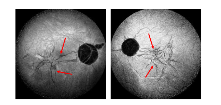
Indocyanine green angiography (ICGA) has been used for visualizing linear lesions in high myopia and is thought to be superior to fluorescein angiography (FA) [10–12]. As shown in Fig. 1, linear lesions are revealed as hypofluorescent structures in the late-phase ICGA images (indicated by red arrows). Although ICGA images can present linear lesions more clearly than other image modalities, linear lesion segmentation is still challenging because of the following two reasons: (1) The shape of linear lesions is quite complex, including linear, stellate, branching and crisscrossing structures. There is no fixed structure for linear lesions. (2) Linear lesions share the same characteristics with retinal vessels in both spatial structures and gray levels.
Fig. 1.
Linear lesions in ICGA.
Deep convolution neural networks (DCNNs) has been proved to be efficient for image processing including image classification [13,14], image segmentation [15] and object detection [16]. It has achieved success in retinal vessel segmentation, which is somewhat similar to the linear lesion segmentation. Liskowski et al. [17] proposed a deep neural network model to detect retinal vessels in fundus images. The approach outperformed previous vessel segmentation methods on accuracy of classification and area under the ROC curve. Later, Wu et al. [18] proposed a DCNN architecture under a probabilistic tracking framework to extract retinal vessel tree. Fu et al. [19] formulated the vessel segmentation as a boundary detection problem using fully connected CNN model. However, there are few studies on linear lesion segmentation. To our best knowledge, we are the first to apply DCNNs to automatically segment linear lesions. In our previous work [20], a conditional generative adversarial network (cGAN) based method was proposed which achieved reasonable performance. In this paper, a new partial densely connected network is proposed to further improve the segmentation performance. Dice loss and weighted binary cross-entropy loss are added to overcome the data imbalance problem. The contributions of our work are listed as follows:
-We are the first to introduce and improve cGANs for the task of linear lesion segmentation. The result is the best among other compared methods.
-A new partial densely connected network is proposed as the generator of cGANs that tries to encourage the reuse of the features.
-Dice loss and weighted binary cross-entropy loss are added in the loss function to deal with the data imbalance problem.
-The problem is formulated as a three-class segmentation task, so that the network can be trained to learn the differences between linear lesions and retinal vessels.
The rest of the paper is organized as follows. In Section 2, the proposed method is described in detail. In Section 3, the experimental results are given and compared with other methods. In Section 4, conclusions and discussions are presented.
2. Methods
2.1 Conditional generative adversarial networks
GANs and its variations [21,22] have been widely studied in the last four years and have achieved success in many image processing applications, such as inpainting [23], future state prediction [24], image manipulation [25,26] and style transfer [27]. Just as GANs learn a generative model of data, cGANs learn a conditional generative model, where the output image is conditioned on an input image. This makes cGANs suitable for image-to-image translation tasks especially for image segmentation. Based on the conditional information, cGANs can generate images with high quality.
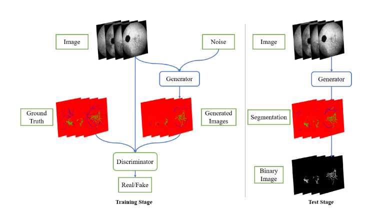
Figure 2 shows the flowchart of the proposed method. In the training stage, the input image and the ground truth are combined in pairs and sent to cGANs to train both the generator and discriminator. ICGA images in the data set are annotated with three class labels: backgrounds, linear lesions and retinal vessels. Since the original two-class segmentation of linear lesions usually segment the retinal vessels as linear lesions, the three-class segmentation can train the networks to learn the differences between linear lesions and retinal vessels and increase the accuracy of segmentation. In the test stage, the generator can generate the three-class segmentation results according to the input images. Finally, retinal vessels and background are combined as the background in the binary segmentation results.
Fig. 2.
Flowchart of the proposed method.
cGANs consist of a generator and a discriminator. During the training process, the generator captures the data distribution and the discriminator estimates the probability that the image comes from the training data rather than the generator. The discriminator learns a loss that tries to detect whether the output image is real or fake while the generator is trained simultaneously.
cGANs learn a mapping from the input image and the random noise vector to the output image . The loss function of cGANs can be expressed as follows:
| (1) |
During iterations, the generator is trained to minimize while the discriminator is trained to maximize , following the min-max optimization rule:
| (2) |
2.2 Partial dense connections in generator
The encoder-decoder model [28,29] has been shown to be one of the most efficient network architectures to complete image segmentation tasks. U-Net [30], one of the typical encoder-decoder networks, is the most common network architecture adopted in generator. The encoder can gradually reduce the spatial dimension of feature maps and capture the long-range information while the decoder can recover object details and spatial dimension. Skip connections are added from the encoder features to the corresponding decoder activations to help decoder layers assemble a more precise output based on features from encoder layers.
However, the original U-Net has poor performance on linear lesion segmentation reported in our previous work [20], because linear lesions and other structures such as retinal vessels are too similar to be distinguished by the network. In the proposed method, partial dense connections are introduced into the U-Net structure in the generator.
Dense connections are first proposed in densely connected convolutional networks (DenseNets) [31], which is the improved network of ResNets [13]. DenseNets obtain significant improvements over the state-of-the-art on most data sets. According to [31,32], DenseNets can drastically reduce the vanishing of gradient because features are reused by creating short paths from early layers to later layers. DenseNets allow layers to access feature maps from all of its preceding layers. As an improvement to DenseNet, TiramisuNet [33] extends the DenseNet architecture to fully convolutional networks for semantic segmentation, while mitigating the feature map explosion. It can complete semantic segmentation efficiently and achieve state-of-the-art results on urban scene benchmark data sets.
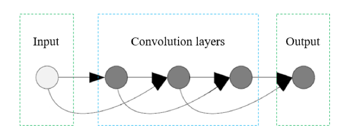
Experiments have shown that although the final classification layer uses weights across the entire dense block, there seems to be a concentration towards final feature-maps, suggesting the adjacent layers might contribute most to the final feature maps [31]. Thus, partial dense connections are proposed and applied on the generator of cGAN in our method. Compared with the original dense connections, long range connections are removed to reduce the training time and increase the computation efficiency, while short range connections are kept to encourage the reuse of the features. By adding partial dense connections, the network can learn the differences between object and background in a relatively short time. The proposed partial dense connections are illustrated in Fig. 3, where each layer makes use of feature maps produced by the previous two layers. The output of the layer is denoted as follows:
| (3) |
where represents the non-linear transformation in the layer, including batch normalization, rectified linear units, pooling or convolution. As each layer has different feature resolutions, we down-sample the feature maps with higher resolutions or up-sample the feature maps with lower resolutions before the partial dense connections.
Fig. 3.
Example of the proposed partial dense connections.
Finally, the encoder-decoder architecture with partial dense connections is used in the generator as shown in Fig. 4. The skip connections share the information between encoders and decoders to make the output much more reasonable. Partial dense connections encourage the reuse of the feature maps so that networks can distinguish the features of linear lesions from those of retinal vessels. Meanwhile, partial densely connected networks have fewer computations than fully densely connected networks. It can finish the training process in a much shorter time.
Fig. 4.
Architecture of generator.
2.3 PatchGAN in discriminator
PatchGAN [22] is employed in the discriminator as shown in Fig. 5. Traditional discriminator in cGANs for image segmentation outputs a single number between 0 to 1 to represent the probability that the output image is real or fake. In contrast, patchGAN tries to classify if each patch in the output image is real or fake. We run this discriminator across the whole output image convolutionally and average all responses to fetch the ultimate discrimination of the output image. As shown in Fig. 5, each pixel in the final layer reflects the possibility of the corresponding patch in the input images.
Fig. 5.
Architecture of discriminator.
By running patchGAN, the size of patches can be much smaller than the full size of the image and it has fewer parameters than the original discriminator. Therefore, it can be applied on arbitrary size images with higher computational efficiency.
2.4 Improved loss function
Previous improvement approaches [22,23] for cGANs have found it beneficial to mix cGAN loss with a traditional loss, such as L1 loss. By adding L1 loss, the discriminator’s task remains unchanged, but the generator is tasked to produce not only undistinguishable images but also images much more similar to the ground truth. We also adopt the following L1 loss in the proposed method:
| (4) |
To improve the segmentation performance of our proposed networks, the Dice loss [34] and the weighted binary cross-entropy loss are also added in the final loss function.
In ICGA images, linear lesions usually occupy a relatively small part of the whole image. The imbalance between the pixel number of background and object often causes the training process to get trapped in a local minimum of the final loss function. The networks usually produce predictions which are biased to backgrounds. To solve the data imbalance problem, the Dice loss function is added as follows:
| (5) |
where and respectively represent the channel of the ground truth and the prediction, and denotes the weight of the Dice loss from the channel. Different weights are allocated to the Dice loss from different channels so that the networks can finally achieve the better linear lesion segmentation.
Although the Dice loss can drastically reduce the data imbalance problem, it still has some limits on the predictions of single pixels. In this paper, the weighted binary cross-entropy loss is added in the final loss function. The Dice loss cares about the intersection area of predictions and the ground truth, while the weighted binary cross-entropy treats the segmentation problem as pixel-wise classification and tries to increase the accuracy of pixel-wise classification for each class. It cannot only highlight the area of linear lesions effectively to enhance the structural information but also balance the gradients of areas in different classes during training. The weighted binary cross-entropy loss is defined as follows:
| (6) |
The total weighted binary cross-entropy is the sum of weighted binary cross entropy calculated in each class. and represent the prediction and the ground truth of the class, respectively. and denote the ratio of object and background.
The final improved loss function is:
| (7) |
3. Experiments and results
3.1 Data set
The medical records and ICGA database of Shanghai General Hospital from April 2017 to August 2017 were searched and reviewed. Totally 76 eyes with linear lesions from 38 subjects were included and imaged (indocyanine green as fluorescer, Heidelberg Retina Angiography 2, Heidelberg Engineering, Heidelberg, Germany, 768 × 768 pixels). The collection and analysis of image data were approved by the Institutional Review Board of Shanghai General Hospital and adhered to the tenets of the Declaration of Helsinki. An informed consent was obtained from each subject to perform all the imaging procedures.
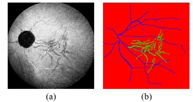
Previous studies [3] show that lacquer cracks are hypofluorescent in the late ICGA phase, which is 15 minutes after ICG dye injection. In our experiments, images were fetched 30 minutes after injection to ensure linear lesions were clear. Due to the small number of subjects, 2 images from each eye are used in the data set. These 2 images have slight differences in the position and intensity because of the different imaging time. Therefore, each subject has 4 images and a total of 152 ICGA images are included in the data set. We randomly split the data set into 4 parts, which contains images from 10, 10, 9 and 9 subjects, for the four-fold cross validation. As shown in Fig. 6, each image in the data set is annotated pixel-wise with three class labels, namely background, linear lesions and retinal vessels.
Fig. 6.
Example of ICGA image data set. (a) An original ICGA image. (b) The annotation of the ICGA image (a). Red regions present the background. Green regions indicate linear lesions and blue regions indicate retinal vessels.
3.2 Evaluation metrics
As each evaluation metric has its own bias toward the specific properties of the segmentation, multiple metrics should be covered to achieve the overall evaluation for the segmentation. To make the results clear and quantitative, we adopt metrics in Table 1 to evaluate our segmentation.
Table 1. Evaluation metrics adopted in the experiments.
| IoU | TP/(TP + FP + FN) |
| DSC | 2TP/(2TP + FP + FN) |
| Accuracy | (TP + TN)/(TP + FP + TN + FN) |
| Sensitivity | TP/(TP + FN) |
| Specificity | TN/(FP + TN) |
(IoU: Intersection over union; DSC: Dice similarity coefficient;
TP: True positive; FP: False positive; TN: True negative; FN: False negative)
Since the linear lesions are our final segmentation object, retinal vessels and background in the three-class segmentation results are combined as the background in the final binary images. Intersection over union (IoU), also known as Jaccard index, is the main metric which measures the overlap between the ground truth and segmentation results [15]. Dice similarity coefficient (DSC) can also be used for comparing the similarity between the ground truth and results [35,36]. Accuracy is another common metric, representing a ratio between the amount of properly segmented pixels to the total pixel number [37]. Furthermore, because the automatic linear lesion segmentation is used to assist doctors in diagnosis and analysis of high myopia, sensitivity and specificity are also included [38].
3.3 Comparison of model variations
In this section we investigate the effect of the partial densely connections and the improvement of the loss function including Dice loss and weighted binary cross-entropy loss.
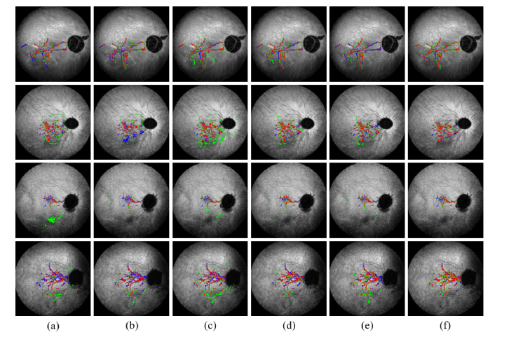
As shown in Fig. 7 and Table 2, the original cGAN method cannot learn the differences between linear lesions and retinal vessels. Partial dense connections and the improved loss function drastically improve the performance of segmentation. Compared with the traditional U-Net generator, generator with partial dense connections encourages the feature reuse during the training process. It can easily capture the main features of linear lesions and learn the differences between linear lesions and retinal vessels. Partial dense connections can also retain the full structure of linear lesions and present more details. Additionally, the Dice loss and the weighted binary cross-entropy loss can solve the data imbalance problem to a great extent, since linear lesions are always slim and only occupy a small part of the image. The improved loss function can avoid the bias to background effectively.
Fig. 7.
Segmentation results by model variations. Green regions present the segmentation results and blue regions present the ground truth. Red regions indicate the intersection between the ground truth and segmentation results. (a) Results of cGAN. (b) Results of cGAN + Dice. (c) Results of cGAN + wBCE. (d) Results of cGAN + Dice + wBCE. (e) Results of cGAN + partial dense connections. (f) Results of the proposed networks. (Dice: Dice loss; wBCE: weighted binary cross-entropy loss)
Table 2. Segmentation results of comparison experiments on model variations, measured with mean and standard deviation.
| Methods | IoU(%) | DSC(%) | Accuracy(%) | Sensitivity (%) | Specificity (%) |
|---|---|---|---|---|---|
| cGAN | 36.53 ± 6.38 | 52.82 ± 7.10 | 98.44 ± 0.22 | 58.91 ± 6.73 | 99.16 ± 0.10 |
| cGAN + Dice [20] | 37.44 ± 5.48 | 53.97 ± 5.93 | 98.52 ± 0.33 | 55.80 ± 7.02 | 99.28 ± 0.24 |
| cGAN + wBCE | 38.71 ± 5.25 | 55.52 ± 5.50 | 98.20 ± 0.35 | 70.98 ± 8.78 | 98.70 ± 0.35 |
| cGAN + Dice + wBCE | 42.61 ± 5.13 | 59.24 ± 5.19 | 98.58 ± 0.32 | 67.16 ± 8.76 | 99.16 ± 0.26 |
| cGAN + PDC | 40.70 ± 2.67 | 57.61 ± 2.74 | 98.52 ± 0.42 | 63.29 ± 8.14 | 99.16 ± 0.30 |
| cGAN + PDC + Dice + wBCE | 52.95 ± 1.22 | 69.21 ± 1.04 | 98.92 ± 0.34 | 77.63 ± 2.23 | 99.29 ± 0.26 |
(Dice: Dice loss; wBCE: weighted binary cross-entropy loss; PDC: partial dense connections)
3.4 Comparison to other deep learning networks
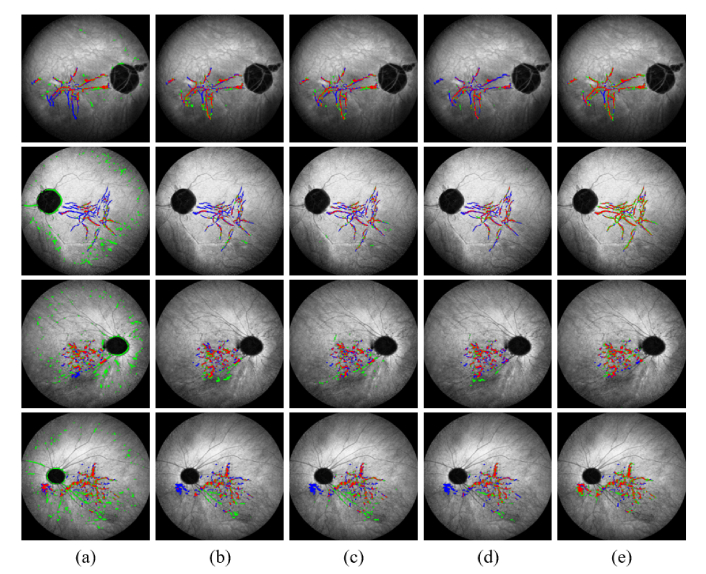
To evaluate the performance of our method objectively, the proposed method is compared with several popular deep learning networks. As shown in Fig. 8 and Table 3, the proposed method obtains the best performance according to all evaluation metrics. Compared to other deep learning networks, it is clear that the adversarial mechanism in cGAN has remarkable performance in linear lesion segmentation. U-Net with partial dense connections are added in the comparison. As we can see, it performs better than original U-Net, PSPNet and TiramisuNet, which not only indicates that the U-Net with partial dense connections can improve the performance of generator, but also represents the proposed method is good at linear lesion segmentation even without cGAN mechanism.
Fig. 8.
Segmentation results on other deep networks. Green regions present the segmentation results and blue regions present the ground truth. Red regions indicate the intersection between the ground truth and segmentation results. (a) Results of U-Net. (b) Results of PSPNet. (c) Results of TiramisuNet. (d) Results of U-Net + partial dense connections. (e) Results of the proposed method.
Table 3. Segmentation results of comparison experiments on other deep networks, measured with mean and standard deviation.
| Methods | IoU(%) | DSC(%) | Accuracy(%) | Sensitivity(%) | Specificity(%) |
|---|---|---|---|---|---|
| U-Net [30] | 12.98 ± 3.53 | 22.80 ± 5.68 | 95.04 ± 0.82 | 30.50 ± 9.69 | 96.64 ± 0.93 |
| PSPNet [39] | 35.98 ± 5.44 | 52.69 ± 5.86 | 97.80 ± 0.27 | 51.42 ± 9.68 | 98.96 ± 0.20 |
| TiramisuNet [33] | 42.15 ± 4.92 | 59.14 ± 4.84 | 98.08 ± 0.34 | 57.44 ± 6.89 | 99.09 ± 0.25 |
| U-Net + PDC | 42.32 ± 3.04 | 59.41 ± 2.97 | 98.29 ± 0.23 | 55.59 ± 8.27 | 99.29 ± 0.16 |
| Proposed | 52.95 ± 1.22 | 69.21 ± 1.04 | 98.92 ± 0.34 | 77.63 ± 2.23 | 99.29 ± 0.26 |
(PDC: partial dense connections)
We also infer that the Dice loss and the weighted binary cross-entropy loss play a big role in achieving the good results, because other networks such as PSPNet and TiramisuNet, designed for natural object segmentation, only use the cross-entropy loss. To make the networks suitable for medical image segmentation, loss functions should be improved to correspond to the object since each part of the loss function has different bias to drive the prediction. Exploring the appropriate loss functions is very important to achieve good segmentations in ICGA images.
4. Conclusions and discussions
With the increasing prevalence of myopia, high myopia has become a main vision-threat. Since the development of linear lesions can reflect the severity of high myopia, it is important and meaningful to achieve automatic linear lesion segmentation. This paper has proposed an improved cGAN framework to segment linear lesions in ICGA images. On one hand, partial dense connections are added in the generator to emphasis feature reuse and to allow the network to better learn the differences between object and background. On the other hand, the final loss function is improved with the Dice loss and the weighted binary cross-entropy loss. They both help to avoid the drastic reductions in accuracy due to the data imbalance problem. Moreover, binary cross-entropy loss helps to classify pixels on the edge of object much more precisely. The proposed networks improved with partial dense connections and additional loss functions can effectively solve the linear lesion segmentation problem. Compared with other popular deep learning networks for image segmentation, our method achieves the better results.
Considering the low image quality, it is difficult to capture the features of linear lesions only via image intensity in ICGA images. Even the ground truth may not be 100% correct. Most diagnosis from experts are based on abundant experiences, which is hard for the networks to learn and conclude. This may explain the low IoU ratios of all methods in our comparison.
In the future work, the segmentation performance can be improved from the following two aspects. First, the data set we used is quite small, which contains only 152 images. We will enlarge the ICGA data set to make the network more generalized. Data augmentation can be an efficient way to increase the size of data set and reduce the over-fitting problem. On the other hand, the data imbalance between object and background still affects the accuracy of segmentation, though Dice loss and weighted binary cross-entropy loss are added to the loss function. Linear lesions are so small that it is difficult for the network to learn the overall structure and shape of the linear lesions. Thus, small errors in the results may lead to drastically reduction in the IoU ratio. To overcome this problem, we will cut the input images into small patches and only keep the patches with the object in the training stage so that the network can fully learn the features of linear lesions.
Funding
The National Basic Research Program of China (973 Program) (2014CB748600); the National Natural Science Foundation of China (NSFC) (61622114, 81401472, 61401294, 81371629, 61401293, 61771326); Collaborative Innovation Center of IoT Industrialization and Intelligent Production, Minjiang University (No. IIC1702).
Disclosures
The authors declare that there are no conflicts of interest related to this article.
References
- 1.The impact of myopia and high myopia: Report of the Joint World Health Organization-Brien Holden Vision Institute Global Science Meeting on Myopia (World Health Organization, 2017).
- 2.Ohno-Matsui K., Yoshida T., Futagami S., Yasuzumi K., Shimada N., Kojima A., Tokoro T., Mochizuki M., “Patchy atrophy and lacquer cracks predispose to the development of choroidal neovascularisation in pathological myopia,” Br. J. Ophthalmol. 87(5), 570–573 (2003). 10.1136/bjo.87.5.570 [DOI] [PMC free article] [PubMed] [Google Scholar]
- 3.Shinohara K., Moriyama M., Shimada N., Tanaka Y., Ohno-Matsui K., “Myopic stretch lines: linear lesions in fundus of eyes with pathologic myopia that differ from lacquer cracks,” Retina 34(3), 461–469 (2014). 10.1097/IAE.0b013e3182a6b494 [DOI] [PubMed] [Google Scholar]
- 4.Wang N. K., Lai C. C., Chou C. L., Chen Y. P., Chuang L. H., Chao A. N., Tseng H. J., Chang C. J., Wu W. C., Chen K. J., Tsang S. H., “Choroidal thickness and biometric markers for the screening of lacquer cracks in patients with high myopia,” PLoS One 8(1), e53660 (2013). 10.1371/journal.pone.0053660 [DOI] [PMC free article] [PubMed] [Google Scholar]
- 5.Ohno-Matsui K., Tokoro T., “The progression of lacquer cracks in pathologic myopia,” Retina 16(1), 29–37 (1996). 10.1097/00006982-199616010-00006 [DOI] [PubMed] [Google Scholar]
- 6.Ikuno Y., Sayanagi K., Soga K., Sawa M., Gomi F., Tsujikawa M., Tano Y., “Lacquer crack formation and choroidal neovascularization in pathologic myopia,” Retina 28(8), 1124–1131 (2008). 10.1097/IAE.0b013e318174417a [DOI] [PubMed] [Google Scholar]
- 7.Hirata A., Negi A., “Lacquer crack lesions in experimental chick myopia,” Graefes Arch. Clin. Exp. Ophthalmol. 236(2), 138–145 (1998). 10.1007/s004170050054 [DOI] [PubMed] [Google Scholar]
- 8.Yannuzzi L. A., The retinal atlas (Elsevier Health Sciences, 2010). [Google Scholar]
- 9.Hung K. C., Chen M. S., Yang C. M., Wang S. W., Ho T. C., “Multimodal imaging of linear lesions in the fundus of pathologic myopic eyes with macular lesions,” Graefes Arch. Clin. Exp. Ophthalmol. 256(1), 71–81 (2018). 10.1007/s00417-017-3833-4 [DOI] [PubMed] [Google Scholar]
- 10.Ohno-Matsui K., Morishima N., Ito M., Tokoro T., “Indocyanine green angiographic findings of lacquer cracks in pathologic myopia,” Jpn. J. Ophthalmol. 42(4), 293–299 (1998). 10.1016/S0021-5155(98)00008-2 [DOI] [PubMed] [Google Scholar]
- 11.Quaranta M., Arnold J., Coscas G., Français C., Quentel G., Kuhn D., Soubrane G., “Indocyanine green angiographic features of pathologic myopia,” Am. J. Ophthalmol. 122(5), 663–671 (1996). 10.1016/S0002-9394(14)70484-2 [DOI] [PubMed] [Google Scholar]
- 12.Suga M., Shinohara K., Ohno-Matsui K., “Lacquer cracks observed in peripheral fundus of eyes with high myopia,” Int. Med. Case Rep. J. 10, 127–130 (2017). 10.2147/IMCRJ.S131545 [DOI] [PMC free article] [PubMed] [Google Scholar]
- 13.He K., Zhang X., Ren S., Sun J., “Deep residual learning for image recognition,” In Proceedings of IEEE Conference on Computer Vision and Pattern Recognition (2016), pp. 770–778. [Google Scholar]
- 14.Rong Y., Xiang D., Zhu W., Yu K., Shi F., Fan Z., Chen X., “Surrogate-assisted retinal OCT image classification based on convolutional neural networks,” IEEE J. Biomed. Health Inform. 23(1), 253–263 (2019). 10.1109/JBHI.2018.2795545 [DOI] [PubMed] [Google Scholar]
- 15.Long J., Shelhamer E., Darrell T., “Fully convolutional networks for semantic segmentation,” In Proceedings of IEEE Conference on Computer Vision and Pattern Recognition (2015), pp. 3431–3440. [DOI] [PubMed] [Google Scholar]
- 16.Redmon J., Divvala S., Girshick R., Farhadi A., “You only look once: Unified, real-time object detection,” In Proceedings of IEEE Conference on Computer Vision and Pattern Recognition (2016), pp. 779–788. 10.1109/CVPR.2016.91 [DOI] [Google Scholar]
- 17.Liskowski P., Krawiec K., “Segmenting retinal blood vessels with deep neural networks,” IEEE Trans. Med. Imaging 35(11), 2369–2380 (2016). 10.1109/TMI.2016.2546227 [DOI] [PubMed] [Google Scholar]
- 18.Wu A., Xu Z., Gao M., Buty M., Mollura D. J., “Deep vessel tracking: a generalized probabilistic approach via deep learning,” In Proceedings of International Symposium on Biomedical Imaging (2016), pp. 1363–1367. 10.1109/ISBI.2016.7493520 [DOI] [Google Scholar]
- 19.Fu H., Xu Y., Wong D. W. K., Liu J., “Retinal vessel segmentation via deep learning network and fully-connected conditional random fields,” In Proceedings of International Symposium on Biomedical Imaging (2016), pp. 698–701. 10.1109/ISBI.2016.7493362 [DOI] [Google Scholar]
- 20.Jiang H., Ma Y., Zhu W., Fan Y., Hua Y., Chen Q., Chen X., “cGAN-Based lacquer cracks segmentation in ICGA images,” In Proceedings of Computational Pathology and Ophthalmic Medical Image Analysis (2018), pp. 228–235. [Google Scholar]
- 21.Goodfellow I., Pouget-Abadie J., Mirza M., Xu B., Warde-Farley D., Ozair S., Courville A., Bengio Y., “Generative adversarial nets,” In Proceedings of Advances in Neural Information Processing Systems (2014), pp. 2672–2680. [Google Scholar]
- 22.Isola P., Zhu J. Y., Zhou T., Efros A. A., “Image-to-image translation with conditional adversarial networks,” In Proceedings of IEEE Conference on Computer Vision and Pattern Recognition (2017), pp. 5967–5976. [Google Scholar]
- 23.Pathak D., Krahenbuhl P., Donahue J., Darrell T., Efros A. A., “Context encoders: Feature learning by inpainting,” In Proceedings of IEEE Conference on Computer Vision and Pattern Recognition (2016), pp. 2536–2544. [Google Scholar]
- 24.Wang X., Gupta A., “Generative image modeling using style and structure adversarial networks,” In Proceedings of European Conference on Computer Vision (2016), pp. 318–335. 10.1007/978-3-319-46493-0_20 [DOI] [Google Scholar]
- 25.Zhu J. Y., Krahenbuhl P., Shechtman E., Efros A. A., “Generative visual manipulation on the natural image manifold,” In Proceedings of European Conference on Computer Vision (2016), pp. 597–613. 10.1007/978-3-319-46454-1_36 [DOI] [Google Scholar]
- 26.Ma Y., Chen X., Zhu W., Cheng X., Xiang D., Shi F., “Speckle noise reduction in optical coherence tomography images based on edge-sensitive cGAN,” Biomed. Opt. Express 9(11), 5129–5146 (2018). 10.1364/BOE.9.005129 [DOI] [PMC free article] [PubMed] [Google Scholar]
- 27.Li C., Wand M., “Precomputed real-time texture synthesis with markovian generative adversarial networks,” In Proceedings of European Conference on Computer Vision (2016), pp. 702–716. 10.1007/978-3-319-46487-9_43 [DOI] [Google Scholar]
- 28.Noh H., Hong S., Han B., “Learning deconvolution network for semantic segmentation,” In Proceedings of IEEE International Conference on Computer Vision (2015), pp. 1520–1528. [Google Scholar]
- 29.Badrinarayanan V., Kendall A., Cipolla R., “Segnet: A deep convolutional encoder-decoder architecture for image segmentation,” IEEE Trans. Pattern Anal. Mach. Intell. 39(12), 2481–2495 (2017). 10.1109/TPAMI.2016.2644615 [DOI] [PubMed] [Google Scholar]
- 30.Ronneberger O., Fischer P., Brox T., “U-net: Convolutional networks for biomedical image segmentation,” In Proceedings of International Conference on Medical Image Computing and Computer-Assisted Intervention (2015), pp. 234–241. 10.1007/978-3-319-24574-4_28 [DOI] [Google Scholar]
- 31.Huang G., Liu Z., van der Maaten L., Weinberger K. Q., “Densely connected convolutional networks,” In Proceedings of IEEE Conference on Computer Vision and Pattern Recognition (2017), pp. 2261–2269. [Google Scholar]
- 32.Huang G., Liu S., van der Maaten L., Weinberger K. Q., “CondenseNet: An efficient densenet using learned group convolutions,” In Proceedings of IEEE Conference on Computer Vision and Pattern Recognition (2018), pp. 2752–2761. 10.1109/CVPR.2018.00291 [DOI] [Google Scholar]
- 33.S. Jegou, M. Drozdzal, D. Vazquez, A. Romero, and Y. Bengio, “The one hundred layers tiramisu: Fully convolutional densenets for semantic segmentation,” In Proceedings of Computer Vision and Pattern Recognition Workshops (2017), pp. 1175–1183. [Google Scholar]
- 34.F. Milletari, N. Navab, and S. A. Ahmadi, “V-net: Fully convolutional neural networks for volumetric medical image segmentation,” In Proceedings of Fourth International Conference on 3D Vision (2016), pp. 565–571. 10.1109/3DV.2016.79 [DOI] [Google Scholar]
- 35.Xiang D., Tian H., Yang X., Shi F., Zhu W., Chen H., Chen X., “Automatic segmentation of retinal layer in OCT images with choroidal neovascularization,” IEEE Trans. Image Process. 27(12), 5880–5891 (2018). 10.1109/TIP.2018.2860255 [DOI] [PubMed] [Google Scholar]
- 36.Ju W., Xiang D., Zhang B., Wang L., Kopriva I., Chen X., “Random walk and graph cut for co-segmentation of lung tumor on PET-CT images,” IEEE Trans. Image Process. 24(12), 5854–5867 (2015). 10.1109/TIP.2015.2488902 [DOI] [PubMed] [Google Scholar]
- 37.Jingyun Guo, Weifang Zhu, Fei Shi, Dehui Xiang, Haoyu Chen, Xinjian Chen, “A framework for classification and segmentation of branch retinal artery occlusion in SD-OCT,” IEEE Trans. Image Process. 26(7), 3518–3527 (2017). [DOI] [PubMed] [Google Scholar]
- 38.Chang H. H., Zhuang A. H., Valentino D. J., Chu W. C., “Performance measure characterization for evaluating neuroimage segmentation algorithms,” Neuroimage 47(1), 122–135 (2009). 10.1016/j.neuroimage.2009.03.068 [DOI] [PubMed] [Google Scholar]
- 39.Zhao H., Shi J., Qi X., Wang X., Jia J., “Pyramid scene parsing network,” In Proceedings of IEEE Conference on Computer Vision and Pattern Recognition (2017), pp. 2881–2890. [Google Scholar]


