Assessment of Structural Features in Cryo-EM Density Maps using SSE and Side Chain Z-Scores

Abstract

We introduce a new method for assessing resolvability of structural features in density maps from Cryo-Electron Microscopy (Cryo-EM) using a fitted model. It calculates Z-scores for secondary structure elements (SSEs) and side chains. Z-scores capture how much larger the cross-correlations score (CCS) is for atoms in such features at their placed location compared to the CCS at displaced positions. Z-scores are larger when the structural features are well-resolved, as confirmed by visual analysis. This method was applied to all 66 maps submitted to the 2015/2016 EMDB map challenge. For each map, the fitted model provided by the map committee was used in this assessment. The average Z-scores for each map and fitted model correlate moderately well with reported map resolutions (r²=0.45 for SSE Z-scores and r²=0.56 for side chain Z-scores). Rankings of the submitted maps based on average Z-scores seem to more closely agree with visual analysis. Z-scores can also be used to pinpoint which parts of a model are well-resolved in a map, and which parts of the model may need further fitting or refinement to make the model better match the density.

Introduction

The analysis of density maps produced by cryo-electron microscopy (cryo-EM) can lead to useful insights into the structure and function of proteins and macromolecular complexes. However not all levels of structural features are visible in every map, hindering such analysis. An ongoing challenge is to reliably and consistently quantitate to what degree structural features are actually resolved in Cryo-EM density maps. The gold-standard resolution of a map, calculated from a Fourier Shell Correlation (FSC) plot between two independent reconstructions is often used for this purpose (Henderson et al., 2012). However, due to map resolution heterogeneity and other factors, this number alone may not accurately represent to what degree structural features are visible throughout the map.

Other metrics based on density alone can also estimate the resolution of the map at a local level, e.g. ResMap (Kucukelbir et al., 2014), however such numbers may also not directly indicate if a certain feature (e.g. a beta strand or a side chain) is actually resolved or not. For this purpose, other methods use a fitted model to calculate whether such structural features are resolved. For example, the EMRinger method quantifies to what degree the carbon-β atom in each side chain of the model is resolved, and whether it is in a proper position with respect to the backbone (i.e. rotameric) (Barad et al., 2015). However, using just one atom in this calculation may make it more susceptible to noise, and also it may not be a good indicator on whether the entire side chain is resolved or not. Morever, the EMRinger score does not quantify whether lower-resolution features (e.g. α-helices or β-strands) are resolved.

In this paper, we use Z-scores to quantify the resolvability of features at two levels: 1) at the secondary structure element (SSE) level (alpha helix and beta strand) and 2) at the amino acid side chain level. This extends on our previous work where Z-scores were used to assess the confidence in rigid fitting of models to cryo-EM density maps (Pintilie and Chiu, 2012). The Z-score (or standard score) is a statistical score which gives the number of standard deviations a single sample point is above the mean of other sample points (Larsen and Marx, 2006). Applied here, we calculate how much larger the cross-correlation score (CCS) for a given feature (SSE or side chain) is at its placed position compared to the CCSs of the same feature after small displacements around that position.

Z-scores calculated for SSEs and side chains are inherently local, in that they represent only a small volume of density around the feature. However, we also averaged Z-scores in each fitted model. This allowed us to 1) study how average Z-scores correlate with the reported resolution for the corresponding map, and 2) rank the submitted maps based on average Z-scores. For comparison, EMringer scores were also calculated for the same maps and fitted models, and compared to average side chain Z-scores and reported resolutions.

The targets of this challenges included GroEL (in silico), Beta-Galactosidase, Brome Mosaic Virus (BMV), Apoferritin, T20S Proteasome, TRPV1 Channel, and 80S Ribosome. A total of 66 submitted maps were evaluated and ranked based on SSE and side chain Z-scores calculated using a fitted model corresponding to each map (Lawson et al., 2017). The fitted models provided by the map committee were used in the analysis. They are rigid-body rotated/translated versions of the Protein Data Bank (PDB) entries, listed as references for each target on the challenge web site (http://challenges.emdatabank.org).

We have implemented the Z-score calculations in a new UCSF Chimera plugin (Pettersen et al., 2004), named ModelZ. It allows interactive calculation and visualization of Z-scores. The plugin and a tutorial can be downloaded at https://cryoem.slac.stanford.edu/ncmi/resources/software.

Methods

SSE Z-scores

To calculate Z-scores for secondary structure elements (SSEs), α-helices and β-strands were first identified based on the assignment given to each residue by the ksdssp method in Chimera (Kabsch and Sander, 1983). Then, for each SSE, the backbone atoms (C, N, Cα, O) were translated by a fixed amount (2Å) in X,Y, and Z directions. At each of the 27 positions (including translation of 0,0,0), the cross-correlation between a simulated map of just the backbone atoms and the density map was calculated (the simulated map was generated with the molmap command in Chimera, using the same grid spacing as the map, and a resolution of 3 times the grid spacing). The Z-score for the SSE was then obtained via the following equation:

$$\text{Z} = \left[S_1-\text{Average}\left(S_{2-N}\right)\right] / \text{StdDev} \left(S_{2-N}\right)$$ (1)

In the above, S₁ refers to the cross-correlation score calculated for the backbone atoms when no translation is applied, i.e. T=(0,0,0), and S_2-N are the cross-correlation scores for all other 26 positions with x,y,zϵ[−2,0,2]. Z-scores were calculated only for proteins in submitted models; RNA molecules, e.g. in the Ribosome map, were ignored. For each map and model, the SSE Z-scores obtained for all SSEs in the model were averaged to obtain a single ‘average SSE Z-score’ representing the entire map and model.

Side Chain Z-scores

To calculate the Z-score for a side chain, all the atoms in the side chain were rotated about the Cα-Cβ bond a total of 9 times in 36° increments. Cross correlation scores were calculated at the original position (no rotation) and at rotated positions, between a simulated map including the side chain atoms only and the cryo-EM density map. As for SSEs, the simulated map was generated with the molmap command in Chimera, using the same grid spacing as the map, and a resolution of 3 times the grid spacing. The Z-score for each side chain is calculated with equation (1) above, S₁ being the cross-correlation score for no rotation, and S_2-N being the 9 cross-correlation scores after rotation.

As for SSE Z-scores, side chain Z scores are calculated only for proteins in submitted models, and not for RNA molecules. Side chain Z-scores were also not calculated for glycine and alanine residues, since glycine does have a Cβ atom, and alanine only has the Cβ side chain atom which does not move when rotating as above. For each map and model, all other side chain Z-scores were averaged to obtain a single ‘average side chain Z-score’ representing the entire map and model.

Average Z-score vs. Resolution (r²)

We measured how well the average Z-scores correlate to reported resolutions for the 66 submitted maps. To do this, we applied regression, fitting a mathematical equation which gives one variable as a function of the other (Cohen, 2002). Two types of equations were considered:

$$y = Ax + B$$ (2)

$$y = Aln\left(x\right) + B$$ (3)

In equations (2) and (3), y represents one of the variables (e.g. average Z-score) and x the other (e.g. reported resolution). Equation (2) is often referred to as a linear relationship and to (3) as a logarithmic or log relationship.

In regression, the constants A and B in each equation are found so that all data points combined give the lowest possible squared residual with respect to the corresponding equation. We also calculated the ‘coefficient of determination’ or r² for both equations in each plot. The value of r² is a measure of the ‘goodness of fit’ (Gujarati and Porter, 2008). The values range between 0 and 1, with higher values obtained for stronger correlations.

Results and Discussion

SSE Z-Scores

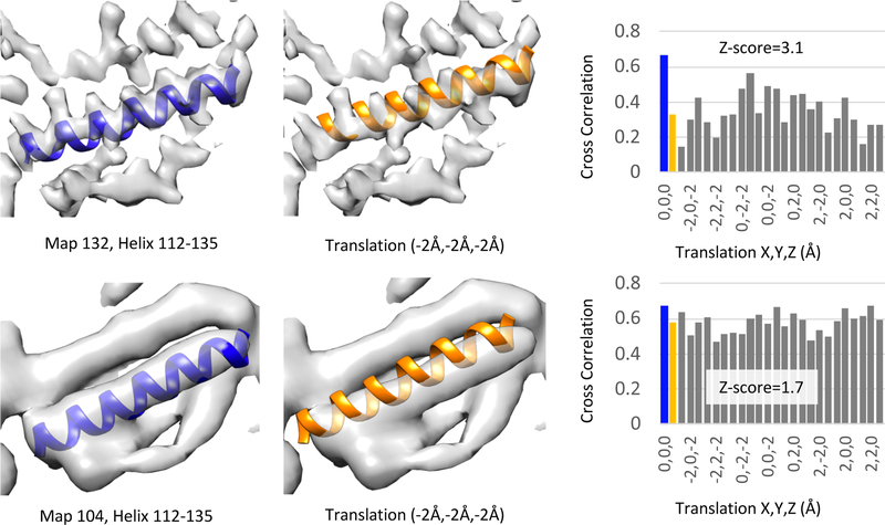
Figure 1 illustrates the calculation of the Z-score for a secondary structure element (an α-helix) in the submitted GroEL maps 132 and 104. For the map of GroEL 132, the reported resolution is 4.1Å. At this resolution, the pitch of helix is typically clear, as shown in Figure 1, top row. When displacing the helix, the cross-correlation score at the new positions is significantly lower than the cross-correlation score at the initial position, and hence the Z-score is quite high (3.1). On the other hand, for the map of GroEL 104, as shown in Figure 1 bottom row, the helix pitch is not well resolved. When translating this helix, the cross-correlation score does not change as much, as shown and plotted in Figure 1, and hence the Z-score is lower (1.7). Interestingly, the reported resolution for this map is 4.4Å, not much lower than that of map 132. In this case, the reported resolution may not be accurate, or the map shown (submitted filtered map) was not high-pass filtered adequately to bring out the finer structural features (Rosenthal and Henderson, 2003).

Figure 1.

Calculation of the SSE Z-score for a helix in submitted map and model 132 (~4.1Å reported resolution), top, and submitted map and model 104 (~4.4Å reported resolution), bottom. On the left, the helix is shown at its actual position, and in the middle image, the helix is shown displaced by −2Å in x,y,z. Cross-correlation scores at original and displaced locations are plotted on the right. A higher SSE Z-score is obtained for the helix in map 132 (3.1) than for the helix in map 104 (1.7), as expected given than the helix appears more resolved in map 132.

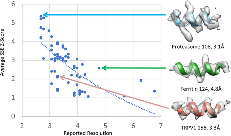
Average SSE Z-scores are plotted for all 66 submitted maps vs. reported resolution in Figure 2. A log relationship, shown with a solid line in the plot, fits the data better (r²=0.45) than linear (r²=0.38). An r² value of 0.45 is moderate, meaning the scores agree in some cases but not all. Three examples are shown on the right in Figure 2. Proteasome 108 has a high reported resolution (3.1Å) and high average SSE Z-score (5.3). A representative helix from the model and the density around it show that indeed the helix is very well resolved, with the helix pitch clearly visible. In some other cases, such as for TRPV1 156, the reported resolution of 3.3Å is high, however a representative helix does not seem as well resolved. The Z-score of 2.1 for the latter is relatively low, well below the average Z-scores for maps at that resolution. On the other hand, the map Apoferritin 124 has a lower reported resolution of 4.8Å, though a relatively high average SSE Z-score of 2.6. A representative helix appears somewhat well resolved, with the helix pitch starting to become visible. Note that in the above examples, we attempted to pick representative helixes which are as well resolved as possible for the given map and model.

Figure 2.

Plot of average Secondary Structure Element (SSE) Z-scores vs. reported map resolution. A log-relationship, solid line, fits the data better (r2=0.45) than linear (r2=0.38). Overall, average SSE Z-score and resolution agree, e.g. Proteasome 108 (right top), where reported resolution and average SSE Z-score are both high; visually the helix shown also appears very well resolved, with the helix pitch clearly visible. On the other hand, TRPV1 156 has a high reported resolution of 3.3Å, though a less resolved helix (bottom right); this helix seems more in line with the one seen in Apoferritin 124 (right middle), with a reported resolution of 4.8Å.

Side Chain Z-scores

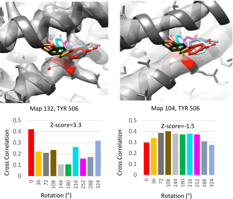
Figure 3 illustrates the calculation of side chain Z-scores for submitted maps GroEL 132 and 104. In the case of map 132, the side chain for this bulky tyrosine residue lies within an area of high density. Rotating the side chain as described above, the cross-correlation score drops significantly at the new positions, and hence a high side chain Z-score is obtained (3.3). In the case of map 104, the side chain lies in density that is very similar to the nearby density. When moving the side chain in this case, similar cross-correlation scores are obtained (some of them are higher), and hence a very low side chain Z-score is obtained (−1.5). These side chain Z-scores thus agree with visual analysis: the side chain is resolved in the case of map 132, but not well resolved in map 104; on the other hand, the reported resolutions are very similar, 4.0Å and 4.4Å respectively, so one might expect that the side chains would be much more similarly resolved.

Figure 3.

Calculation of the side chain Z-score for TYR 506 in submitted maps and models 132 (4.1Å reported resolution) and 104 (4.4Å reported resolution). The original position of the side chains are shown in red; rotated side chains (around Cα-Cβ bond) are shown with other colors. Cross-correlation scores at original and rotated positions are plotted (bottom). The side chain appears resolved in Map 132 with a clear density blob at its initial position, whereas no density for it can be seen in Map 104. Correspondingly, a high Z-score is obtained for the side chain in map 132 (3.3), and a low Z-score is obtained in map 104 (−1.5).

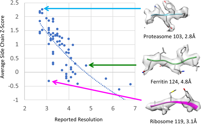
Average side chain Z-scores are plotted for all 66 submitted maps vs. reported resolution in Figure 4. A log relationship fits the data better (r²=0.56) than a linear relationship (r²=0.51). Again, the r² value is moderate, meaning there is some correlation between the two scores but they do not agree in all cases as can be also seen in the plot. Three examples are shown on the right in Figure 4. Proteasome 103 has a high average side chain Z-score (2.2) and high reported resolution (2.8Å). A representative portion of the map and model also show very well resolved side chains (top right). Ribosome 119 has a high resolution estimate of 3.1Å, however a much lower average side chain Z-score of −0.34. A representative segment shows that side chains indeed are not well resolved (bottom right). On the other hand, the submitted map Apoferritin 124 has a lower reported resolution of 4.8Å. It has an average Z-score of 0.2, and visually it seems like side chains are starting to become somewhat resolvable (middle right). Again, we attempted to pick representative segments from each map and model so that they are resolved as well as possible for the given map model. For these examples, much like for SSE Z-scores, average Z-scores seem to more closely indicate how well structural features are resolved in a map, while the reported resolutions may be misleading in some cases.

Figure 4.

Plot of average side chain Z-scores vs. reported map resolution. A log-relationship, solid line, fits the data better (r²=0.56) than a linear relationship (r²=0.51). As with SSE Z-scores, average side chain Z-score and estimated resolution agree in some cases, e.g. Proteasome 103, which has high average side chain Z-score and high reported resolution; visually the side chains also look very well resolved. Ribosome 119 on the other hand has a relatively high reported resolution of 3.1Å, though low average side chain Z-score; visually the side chains are not well resolved. By comparison, Apoferritin 124 has a lower resolution estimate of 4.8Å, though the side chains seem slightly better resolved, as shown, while also having a slightly higher average side chain Z-score.

SSE Z-scores vs. side chain Z-scores

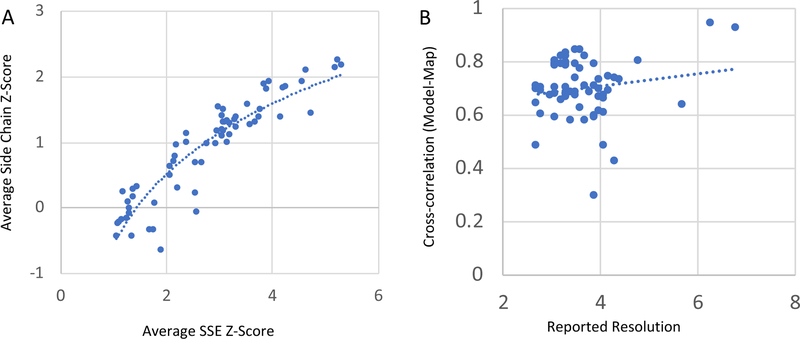
The plot in Figure 5A shows that average SSE Z-scores and side chain Z-scores are strongly correlated (r² = 0.83). So, for any map and model, if the average SSE Z-score is high, then the average side chain Z-score is also likely to be high. This is not surprising since if the backbone is well resolved, then the side chains are also likely to be visible. It is interesting to note however that the correlation is not linear, i.e. as the average SSE Z-score score drops (presumably at lower resolutions), the side chain Z-score starts to drop faster. This indicates that at lower resolutions, where the side chains are no longer discernible, side chain Z-scores level off and SSE Z-scores become more useful. On the other hand, side chain Z-scores are more useful when analysing higher resolution density maps.

Figure 5.

(A) Plot of average side chain Z scores vs. average SSE Z-scores for all 66 submitted maps. There is a strong correlation between the two (r² = 0.83, log relationship). (B) Plot of the cross-correlation between the a simulated map of the model and the map vs. reported resolution. There is very weak correlation between the two (r²=0.02).

Z-scores vs Cross Correlation

When presenting a map and model, it is common practice to report the cross-correlation between the two. However, in our experience, the cross-correlation (CC) score by itself doesn’t seem to correlate strongly with resolution, with higher scores sometimes being observed in lower resolution maps. For example, in Figure 1, the CC for the helix in the map that seems to be lower resolution, 104, is the same as the CC for the helix in the map that seems to be higher resolution (132). To test this further, the CC scores between the entire model and the submitted maps were plotted vs. reported resolution in Figure 5B. The CC was calculated between each submitted map and a simulated density for the entire fitted model. The latter was generated with the Chimera molmap command, at the reported resolution and same grid spacing as the submitted map. The plot shows that cross-correlation scores calculated as such correlate very poorly to the reported resolution (r²=0.02). The cross-correlation score is nonetheless still a very useful score, however it seems to be more meaningful when being compared across different placements of a feature in the same map, as here, or even different placements of the entire model within the same map, as done previously (Pintilie and Chiu, 2012).

Interpretation of SSE and side chain Z-scores

The Z-score as defined equation 1 represents how many standard deviations a score of interest is above the mean of other related scores. We applied it here to cross-correlation scores obtained for features at their placed locations (the score of interest), in relation to other scores where the feature is slightly displaced from this location. When Z-scores are above 0, it indicates that the cross correlation is higher at the placed location than at the displaced positions around that location. On the other hand, if the Z-score is 0 or lower, the score at the placed location is overall the same or lower than at the surrounding locations. This seems to correlate well with whether the feature is resolved and visible in the density map.

For the maps and models analysed here, average SSE Z-scores have a wider range ~(1,6) than average side chain Z-scores ~(−1,2), as plotted in Figure 5. The higher average Z-scores for SSEs are likely due to their larger size in terms of number of atoms; the backbone atoms in an SSE also tend to be stabilized by hydrogen bonds, and hence they are more readily resolvable. On the other hand, individual amino acid residues have fewer atoms than SSEs, and their side chains can have less restricted conformations, and hence are generally harder to resolve.

Side Chain Z-scores per Residue Type

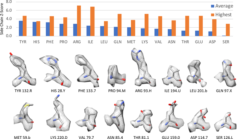
Figure 6 shows the average side chain Z-scores per residue type for the submitted map/model Proteasome 103; larger/bulkier side chains such as tyrosine and histidine tend to have higher Z-scores on average compared to smaller side chains. It is interesting to note that Proline residues also tend to have high average Z-scores. Even though the rotations around the Cα-Cβ bond are not meant to test realistic models of this residue, they seem to be good at detecting whether the density around the residue matches its planar form (as it is shown from the side in Figure 6).

Figure 6.

Top: plot of side chain Z-scores, per residue type, obtained from the submitted map and model Proteasome 103 (reported resolution of 2.8Å). The plot shows the average Z-score (blue), and also the highest Z-score (orange) for each type of residue. The residues with the highest Z-score are shown in the bottom two rows; the labels are formatted as “<residue type> <residue number>.<chain id>“.

Factors affecting Z-Scores

The SSE and side chain Z-scores were calculated using the submitted filtered maps. Post processing in the form of high pass filtering or sharpening helps to bring out higher-frequency components (Rosenthal and Henderson, 2003). We calculated SSE and side chain Z-scores using unfiltered maps; the result was that the Z-scores were lower than when using filtered maps; moreover the correlations between average Z-scores and reported resolution were weaker. Hence, SSE and side chain Z-scores are sensitive to proper post-processing of the reconstructed map. We expect that over-sharpening, which introduces excessive noise, would also lower the Z-scores.

Several parameters were used in calculating Z-scores. One is how much an SSE is displaced in each direction; here we used 2.0Å. We tried small variations around this value (e.g. 1.5–3.0); these did not greatly affect the Z-scores or their correlation to reported resolutions. Another parameter is the angle that side chains are rotated by; here we used 36°, for 10 rotations in total. Variations in this parameter also do not seem to affect Z-scores and correlations. Lastly, a resolution parameter was used for calculating simulated maps (we used 3× the grid spacing of the map); we also tried values of 2×, 3×, and 4× the grid spacing. This also did not greatly affect Z-scores and correlations to reported resolution. (We avoided using the reported resolution in the calculation of the simulated maps, to avoid making the Z-score directly dependent on this number, which might influence the correlation analysis between the two).

Another factor we considered was whether to use the cross-correlation score, or simply the average density at atom positions. Using the average density resulted in lower Z-scores and weaker correlations reported resolutions. This may be because the cross-correlation score also takes into account where the density is low, away from SSE or side chain atoms, correlating this to density map values, whereas the average density score only looks at density values at atom positions.

Comparison to EMRinger Score

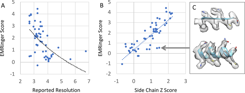
We compared our average side chain Z-scores to EMRinger scores, since they similarly aim to evaluate how well side chains are resolved. We applied the EMRinger method (Phenix version 1.14–3211) to all 66 submitted maps, however it did not return scores for 10 of the maps (111, 119, 131, 134, 136, 137, 140, 142, 146, 152). For the other 56 maps and models, the EMRinger score is plotted vs. the reported resolution in Figure 7A. A weaker correlation between the two is observed (r²=0.31 log, r²=0.28 linear relationships) than for our average side chain Z-scores (r²=0.56 log, r²=0.51 linear). Our average side chain Z-scores correlate relatively well to EMRinger scores overall, (Figure 7B), with r²=0.71 linear relationship, meaning that the scores tend to be similarly high or low for a given map and model. However, there are places where the scores disagree; an example is shown in Figure 7C, which shows two small segments of BetaGal map 106. In this example, EMRinger gives the map a low score by its standards (0.48, max of ~4.5), whereas our average side chain Z-score is moderately high (1, max ~2). A visual inspection of the maps shows side chains are quite well resolved (inset), and hence a higher side chain score seems more appropriate.

Figure 7.

Left, plot of EMRinger score vs. reported resolution (r²=0.31 for log-relationship and r²=0.28 for linear). In the middle, a plot of EMRinger score vs. average side chain Z-Score is shown. The scores correlate well (r²=0.71), though there seem to be some cases in which EMRinger appears to give low score, e.g. BetaGal 106 (resolution 3.1Å, inset) whereas the average side chain Z-score is relatively high. Side chains in this map appear to be quite well-resolved, as shown on the right.

Ranking of maps using side chain Z-scores

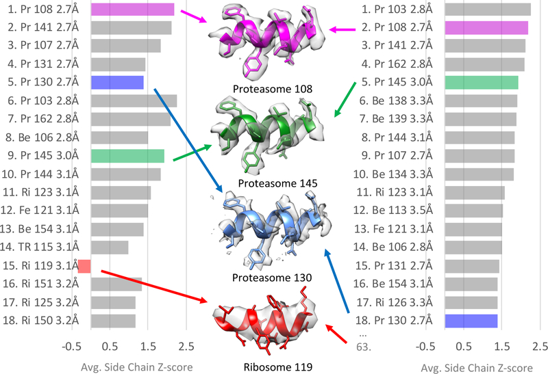
All 66 maps submitted to the challenge were ranked by reported resolution and also average side chain Z-scores, with plots shown in Figure 8. Side chain Z-scores were used instead of SSE Z-scores because most maps were of moderately high resolution (2–5Å). Overall the rankings have the same maps in the top 18, however the ranking by average side chain Z-scores seems to more closely match a visual analysis of the maps, as shown in the center of Figure 8. For example, the map Proteasome 145 seems to have better resolved side chains than the map Proteasome 130, yet it is ranked lower by reported resolution; the ranking by average side chain Z-score seems more appropriate. Also, Ribosome 119 is placed high by reported resolution at #15, though a look at the map reveals that side chains are not well resolved; it is more appropriately ranked #63 by average side chain Z-score.

Figure 8.

Rankings of submitted maps in order of (left) reported resolution, and (right) average side chain Z-score. Target names are abbreviated (Pr – T20S Proteasome, Be – Beta Galactosidase, Ri – Ribosome, Fe – Apoferritin, TR – TRPV1). Some maps with very well-resolved side chains appear in both lists close to the top, e.g. Proteasome 108, and 145. However the reported resolution doesn’t seem to correspond as well to the quality of side chains densities for Proteasome 130 and Ribosome 119. On the other hand, the ranking by average side chain Z-score corresponds well with how well the side chains appear resolved. In the center panel a representative segment from four submitted maps and models are shown.

Using Z-scores for heat maps

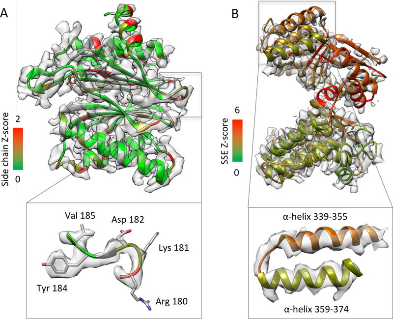
Figure 9 illustrates how SSE and side chain Z-scores can be used to visualize which features in a map are resolved better than others, though at the same time which parts of the model are fitted to the map properly and which parts may need further flexible fitting (Adams et al., 2010; DiMaio and Chiu, 2016; Murshudov et al., 1997; Topf et al., 2008; Trabuco et al., 2009) or refinement (Adams et al., 2010; DiMaio and Chiu, 2016; Murshudov et al., 1997). In Figure 9A, an entire protein from submitted map and model Proteasome 108 is shown, with ribbon coloring corresponding to the side chain Z-score for each residue. A small fragment is shown inset; the bulky Tyr 184 side chain is well resolved and hence has a higher Z-score, while the Arg 180 has much less density around it and hence has a low Z-score.

Figure 9.

Z-scores used as ‘heat maps’. (A) Submitted map and model Proteasome 108, chain 1, is shown with coloring for side chain Z-scores. Many side chains are well-resolved (green color), e.g. Tyr 184, however some are not (red color), e.g. Arg 180. (B) Submitted map and model GroEL 132, chain A, shown with coloring for SSE Z-scores. Some SSEs are better resolved (green) than others (red).

Figure 9B shows the submitted map and model of GroEL 132, in which most side chains are not visible. Here, the ribbon display for the model is colored according to the Z-score of each SSE. The coloring can help identify which SSEs are resolved better than others. For example, amongst the two helices shown inset, the bottom helix seems to be better resolved, with the helix pitch slightly more visible, compared to the top helix. Correspondingly, the bottom helix is more green than the top one, since it has a higher Z-score.

Conclusions

Assessment of models built de-novo based on high resolution cryo-EM density maps or flexibly-fitted to them is becoming extremely important in the field of structural biology, as important insights are usually derived based on such models. In this paper we have applied the calculation of Z-scores to quantitate whether certain structural features are visible in density maps obtained by Cryo-EM, an important step in assessing how confident we can be on the models and hence the derived insights. As we would hope, the scores correlate reasonably well to reported resolutions, however they seem to produce a more reliable indication of how well structural features are actually resolved. Average Z-scores produce rankings that more closely matches visual analysis. The scores do however depend on having a properly fitted model, and thus can also indicate where the model needs further fitting or refinement. Such quantification is very useful for the investigators to articulate any mechanistic model or to plan future experiments to probe for structure function relationship of the proteins under investigation.