Selection of Fitting Model and Arterial Input Function for Repeatability in Dynamic Contrast-Enhanced Prostate MRI

Abstract

Rationale and Objectives:

Analysis of Dynamic Contrast-Enhanced MRI is notable for the variability of calculated parameters. The purpose of this study was to evaluate the level of measurement variability and error/variability due to modeling in DCE MRI parameters.

Materials and Methods:

Two prostate DCE scans were performed on 11 treatment-naïve patients with suspected or confirmed prostate peripheral zone cancer within an interval of less than two weeks. Tumor-suspicious and normal-appearing regions of interest in the prostate peripheral zone were segmented. Different Tofts-Kety based models and different arterial input functions (AIFs), with and without bolus arrival time (BAT) correction, were used to extract pharmacokinetic parameters. The percent repeatability coefficient (%RC) of fitted model parameters K_trans, v_e, and k_ep was calculated. Paired t-tests comparing parameters in tumor-suspicious ROIs and in normal-appearing tissue evaluated each parameter’s sensitivity to pathology.

Results:

Although goodness-of-fit criteria favored the 4-parameter extended Tofts-Kety model with the BAT correction included, the simplest 2-parameter Tofts-Kety model overall yielded the best repeatability scores. The best %RC in the tumor-suspicious ROI was 63% for k_ep, 28% for v_e and 83% for K_trans. The best p-values for discrimination between tissues were p<10⁻⁵ for k_ep and K_trans, and p=0.11 for v_e. Addition of the BAT correction to the models did not improve repeatability.

Conclusion:

The parameter k_ep, using an AIF directly measured from blood signals, was more repeatable than K_trans. Both K_trans and k_ep values were highly discriminatory between healthy and diseased tissues in all cases. The parameter v_e had high repeatability but could not distinguish the two tissue types.

Introduction

Dynamic contrast enhanced (DCE) MRI can potentially differentiate tumor vasculature from a normal blood vessel network by measuring vascular permeability and perfusion. There is a wide consensus that the use of quantitative DCE MRI could have a role in the clinical practices for determining disease recurrence and for evaluation of response to neoadjuvant drug therapy in cancer. DCE MRI has been validated as a surrogate marker of tumor angiogenesis in prostate cancer (1,2). Existing evidence shows that pharmacokinetic DCE parameters can provide a good measure of response in Androgen Deprivation Therapy for prostate cancer (3) and a good indicator of isolated limb perfusion treatment response in soft tissue sarcomas (4).

To determine the usefulness of a biomarker, it is necessary to understand its variability (intra-subject, inter-subject, etc.). Intra-subject variability can be measured using two scans of the patient without intervening therapy. Modeling and analysis of DCE is disappointingly notable for the variability of calculated parameters - both between patients and between studies. This is in part due to the fact that DCE analysis is sensitive to the variety of acquisition and analysis choices that need to be made and parameters to be selected (5,6). Some of the sources of uncertainty pertain to the particular scanner, radio frequency coil homogeneity/shimming, and the pulse sequence used to acquire the images. Other sources of variability include the analysis software, the pharmacokinetic (PK) model used, the presence or absence of T₁ mapping, and the presence or absence of time series image registration (5).

One critical input to quantitative DCE calculations is the arterial contrast agent time-dependent concentration curve, also called the arterial input function (AIF). Uncertainty in the AIF is arguably the greatest contributor to measurement error (7).

The choice of AIF determination, including the choice of source vessel, can lead to significant differences in the values of the estimated PK parameters (8), as also shown by McGrath et al. who used data from repeated DCE-MRI acquisitions in a preclinical tumor rat model to quantify the sensitivity of tracer kinetic modeling parameters to the form of the AIF (9).

Often the AIF is calculated from the DCE signal in an artery in the image field of view. There are a number of problems associated with this approach. When contrast agent concentrations are large (e.g., within vessels) signal intensity varies nonlinearly with contrast agent concentration, making it difficult to assess concentration. The calculation of contrast concentration is also affected by the intrinsic T₁, which is difficult to directly measure in blood. Lu et al. found that the longitudinal relaxivity R₁ (=1/T₁) of arterial blood at 3T depends on hematocrit and can be approximately described as following the linear relationship: R₁ = 0.52 Hct + 0.38, valid in the normal hematocrit (Hct) range 0.38–0.46 (10). According to this equation, with the given range of Hct, peak blood contrast concentrations anywhere between 6.5 and 9.1 mM/l could be calculated from the same example of blood signal. Slight anemia or polycythemia could increase the uncertainty further. Other systemic problems with evaluating the AIF concentration from a vessel in the field of view are partial volume effects, in-flow effects, flow-profile dependency, T₂* effects, and temporal undersampling causing underestimation of the peak value (11,8). Any error in the amplitude of the AIF directly affects the calculated pharmacokinetic parameters - K_trans and v_e have been shown to scale nearly proportionally with the AIF (12), and the choice of source vessel can change their calculated values (13).

Due to the many problems with estimating the AIF from an artery in the image field of view, sometimes a predefined functional form or population-averaged AIF is used (11). This choice of AIF obviously cannot account for differences between patients or even between scans of the same patient in cardiac output and injection rates. Ashton et al. evaluated the scan-rescan coefficient of variation for repeated scans of 25 patients with solid tumors in the liver and compared a data-derived AIF with a model AIF. Using the data-derived AIF reduced the scan-rescan coefficient of variation in K_trans by 70% in liver lesions (14). In prostate cancer, Azahaf et al. found that one particular population AIF worked better than another in generating values of K_trans that could discriminate between malignant and benign tissue, and that it provided better or equal discrimination compared to an individually measured AIF (15).

Normalizing AIFs has also been investigated. AIF-caused variations in measured parameters were reduced when reference-tissue-adjusted AIFs were used (16). In that study an ROI in the adjacent obturator muscle area on the same image slice as the tumor ROI was used as a reference tissue for AIF amplitude adjustment. The AIF amplitude was adjusted until the Tofts Model fitting of the muscle ROI DCE-MRI data returned a v_e value of 0.1, which is within the range of literature-reported values.

If the AIF is measured in a large artery upstream from the tissue of interest, further downstream the concentration is likely to be both delayed and dispersed. Ignoring a possible shift in bolus arrival time (BAT) has been shown to degrade the fit quality in DCE modeling (17), while incorporation of a BAT shift has shown improved reproducibility of calculated model parameters (18). When using a functional form for the AIF or one derived from a population, it is likely that there be an even greater need for the bolus arrival time (BAT) to be part of the fitting process, due to variations in injection timing.

This work sets out to investigate the practical utility of DCE derived quantitative biomarkers by comparing the repeatability of pharmacokinetic parameters calculated using different models and analysis methods. In contrast to previous work on the subject of model and AIF choices in DCE, here the focus is on the within-patient stability of parameter estimates, i.e., on repeatability under conditions of unavoidable measurement error. We vary the pharmacokinetic model, the AIF determination approach, and whether a BAT shift calculation was included. While determination of the ground truth AIF is difficult to achieve in practice, analysis of the AIF choices in a scan-rescan dataset provides us with a unique setting to optimize those choices such that repeatability is increased.

Although repeatability is a critical characteristic of a biomarker for treatment response or disease progression studies, the sensitivity of a biomarker to tissue changes such as may be reflected in different values for healthy and diseased tissue, is also important. For this reason the parameters calculated from the analysis methods were also tested for their discriminatory ability between areas of suspected malignancy and areas categorized as healthy.

Materials and Methods

Image acquisition and annotation

The cohort analyzed in this study is a subset of patients (n=11) from a population (n=15) participating in a multiparametric MRI repeatability study of prostate CA (19). Four patients out of the original 15 on whose DCE scans a tumor-suspicious region could not be identified were excluded. The work described was carried out in accordance with the World Medical Association Declaration of Helsinki Ethical Principles for Medical Research Involving Human Subjects. Institutional review board approval was obtained for this Health Insurance Portability and Accountability Actcompliant study. Written informed consent was obtained from the study participants. Two clinical prostate 3D DCE scans were performed on treatment-naïve patients within an interval of less than two weeks on a General Electric 3T scanner using a receive endorectal coil. 0.15 mmol/kg gadopentetate dimeglumine (Magnevist, Berlex Laboratories, Wayne, New Jersey) was injected intravenously using a syringe pump at the rate of 3 ml/s followed by 20 ml saline flush at the same rate (Figure 1). The clinical pulse sequence parameters varied between patients but were in the range: TR 3.7–4.1 ms; flip angle 12° or 15°; TE=1.3–1.4 ms; time per frame 5–8.4 s; scan time 4.5 – 5.5 min; matrix either 256 × 256 × 16 with resolution 1 × 1 × 6 mm, or 512 × 512 × 32 with resolution 0.55 × 0.55 × 2.5 mm.

Figure 1.

Typical images of prostate appearance after contrast injection. Shown from left to right are cropped frames #6,#7,#8,#9,and #19. The time between frames was 7.3 sec.

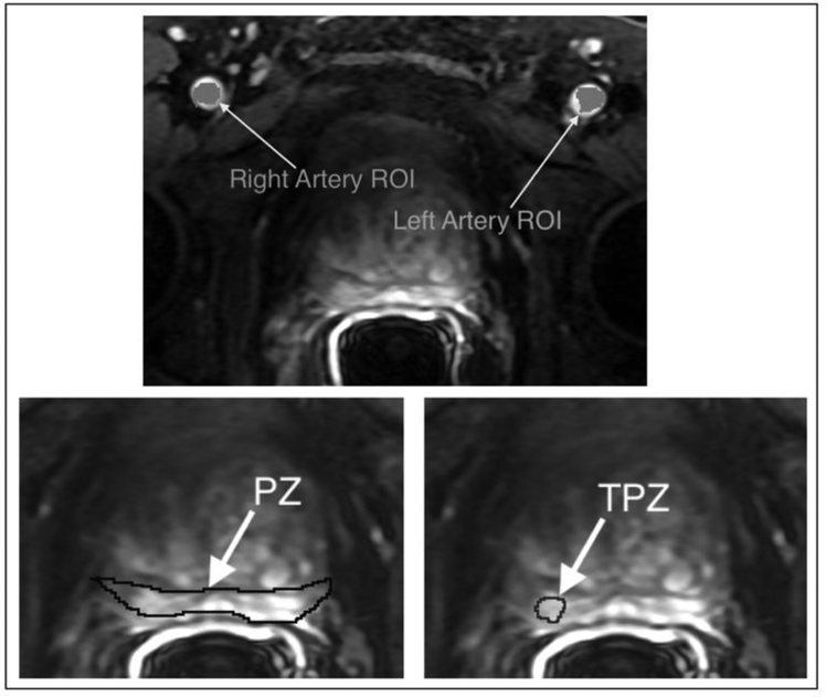
The MRI studies were deidentified and presented in a random order to an experienced abdominal radiologist (##) who assigned a Prostate Imaging Reporting and Data System (PI-RADS v2) score (20) to each study. Using 3D Slicer software (http://slicer.org ) the same radiologist segmented three regions of interest (ROIs) on the DCE difference image (subtraction of baseline pre-contrast images from post-contrast first bolus arrival phase images). As illustrated in Figure 2, these three regions were defined as follows:

1. A Peripheral zone tumor-suspicious region of interest (TPZ). The sector containing the lesion was noted. Mean TPZ ROI sizes are shown in Table 1, as are the percentage of the peripheral zone represented by the TPZ ROI.

2. The whole peripheral zone ROI (PZ). In all the following analyses, NPZ refers to ‘normal-appearing’ peripheral zone, i.e. the whole peripheral zone PZ excluding the tumor-suspicious zone TPZ.

3. Left Femoral Artery (LA) and Right Femoral Artery (RA) voxels.

Figure 2.

Examples of regions of interest (ROIs) that were identified and segmented by an experienced abdominal radiologist on each DCE difference image: left artery voxels and right artery voxels for AIF measurement; whole peripheral zone (PZ); and peripheral zone tumor-suspicious ROI (TPZ).

Table 1:

Patient-level summary of clinical indications for MR imaging, histopathology, PSA and PI-RADS v2 assessment of the disease in the evaluated cohort, mean suspected tumor ROI size (mean of segmentations in two repeated MRI scans ± standard deviation), and % tumor volume of peripheral zone (mean of two repeated scans ± standard deviation).

Subject #	Indication for the MRI exam	Max. Gleason at biopsy	PSA ng/ mL	PI-RADS v2 Scan I	PI-RADs v2 Scan II	Suspected tumor ROI: size (mm3)	Suspected tumor ROI: % volume of PZ
1	Known PCa, staging	3+4	5.4	4	4	378±336	4.5±3.7
2	Known PCa, assess change	3+4	7.5	2	3	469±117	3.8±0.2
3	Known PCa, staging	3+3	8.2	4	4	794±190	6.3±0.8
4	Known PCa, staging	3+3	4.3	2	2	89±50	1.3±0.8
5	Elevated PSA, staging	4+5	6.2	4	4	663±367	8.7±0.5
6	Known PCa, assess change	3+3	4.8	4	4	499±170	3.6±1.8
7	Elevated PSA, staging	Benign	9.4	4	4	541±20	4.4±0.6
8	Known PCa, assess change	3+3	3.15	4	4	82±19	1.1±0.3
9	Known PCa, assess change	3+3	9.7	4	4	530±109	4.2±0.6
10	Elevated PSA, staging	Benign	5.5	3	4	112±49	2.2±0.8
11	Known PCa, staging	3+4	4.16	4	3	340±44	2.6±0.2

The segmentations were performed while simultaneously viewing the T₂ and diffusion-weighted images from the same patient study. Participating patient details are shown in Table 1. There was good agreement in the locations of the suspected tumor ROI areas, which was assessed by a separate reader by comparing the noted lesion sector between the baseline and repeat studies. The size of the suspected tumor ROI did, in some cases, differ between the baseline and repeat study, as shown in Table 1.

Model analysis

First, the MRI signal from the prostate and from blood was converted to longitudinal relaxivity under the condition of a low-flip angle gradient-echo sequences, with knowledge of θ and TR - the flip angle and repetition time respectively. The conversion from longitudinal relaxivity, R₁, to time-dependent contrast concentration, C(t), is assumed linear and was done via this equation: R₁(t)=r₁.C(t)+R₁₀, where r₁ is the relaxivity of the contrast agent used, and R₁₀ is the longitudinal relaxivity of the tissue without added contrast agent. Here T₁₀ of prostate tissue was assumed constant at 1434 ms (21). The arterial T₁₀ of blood was estimated as 1630 ms according to the equation T₁₀ = 1/(0.52 Hct + 0.38)as suggested in (10), assuming Hct=0.45.

The AIF estimation methods (designated AIF1, AIF2, and AIF3 below and in Figures 4–8) evaluated were:

Figure 4.

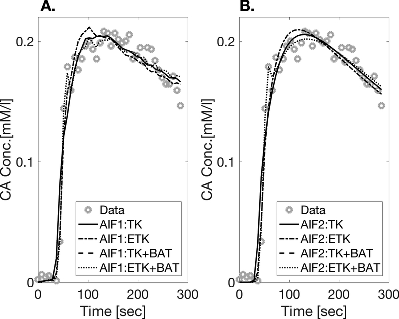
The model fits for a single randomly picked voxel in the TPZ ROI of patient #7: A. PK models with AIF1, B. PK models with AIF2.

Figure 8.

k_ep repeatability (a) and tumor discrimination (b). See Fig. 6 for legend.

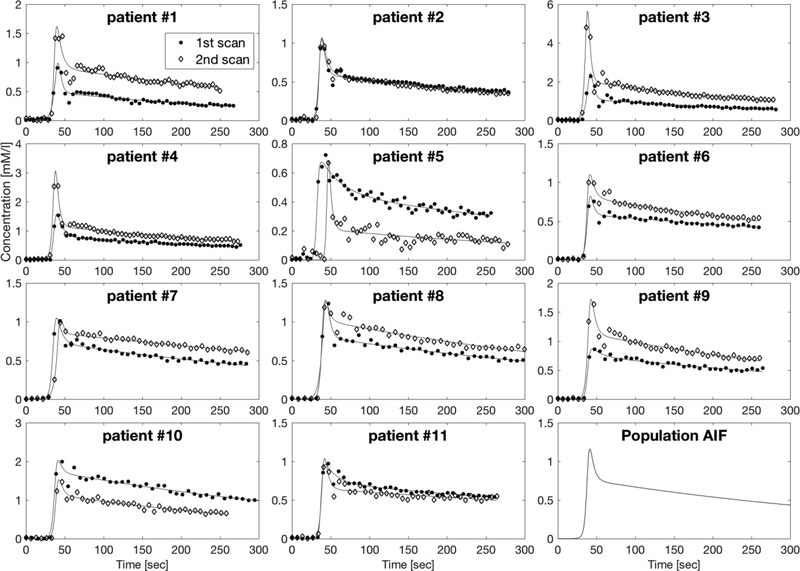
1. AIF1: A plasma concentration AIF calculated from the mean of the measured blood signals in the manually segmented left and right artery voxels: C_p,i(t) for each scan i, shown in Figure 3. The plasma concentration was derived from the blood concentration, C_b(t) using C_p(t) = C_b(t)/(1 - Hct) assuming Hct = 0.45.

2. AIF2: One AIF for all subjects scans, which is the population average of all the measured AIF’s in this study - the injection protocol was typical for our institution. The population average in this case was calculated by first fitting each AIF to a heuristic parameterization – in this case a biexponential multiplied by a sigmoid function - as follows:

   $$Y(t)=Y_{max}[(1-f)e^{\frac{-\left(t-t_0-t_{max}\right)}{{\sigma }_1}}+f{e}^{\frac{-\left(t-t_0-t_{max}\right)}{{\sigma }_2}}]÷[1+e^{\frac{t-t_0-t_{\max }{}_{/2}}{t_{\max /10}}}]$$ [1]

   A biexponential is widely used to describe a bolus injection (22) – and a sigmoid has been used elsewhere to describe the rise from zero of the concentration (22). Figure 3 shows the calculated and fitted AIFs for all scans. The median values of the fitted parameters [t₀, t_max, Y_max, σ₁, σ₂, f ] were then used to construct the population AIF, C_pop(t), shown in the bottom right axes of Figure 3. The resulting population AIF looked qualitatively similar in amplitude and form to the median AIF calculated from a previous study at our institute.

3. AIF3: To counter the possible underestimation of the peak value, the above population AIF (AIF2) was scaled for each DCE acquisition scan j by the normal appearing peripheral zone maximum concentration in that scan max(C_NPZ,j) as follows:

   $$C_{pop,j}(t)=C_{pop}(t)\cdot \max \left(C_{NPZ,j}\right)\cdot \frac{1}{N}{\displaystyle {\sum }_{i=1}^N\raisebox{1ex}{$1$}\!\left/ \!\raisebox{-1ex}{$\max \left(C_{NPZ,j}\right)$}\right.}$$ [2]

   where C_NPZ,j is the average of the voxel signals in the NPZ ROI of scan j.

   Although in this study regions of obturator muscle were also segmented, with the intention to attempt to use its signal for scaling, the enhancement signal in the obturator was generally too noisy to extract a scaling factor.

Figure 3.

AIFs calculated after measurement from the mean of left and right artery ROIs in all 22 DCE scans (11 patients x 2 scans) with fits to biexponential x sigmoid functions (see text). The concentration units of the vertical axis are mM/liter and the horizontal axis is Time [sec]. The population AIF resulting from taking the median values of the parameters fitted to Eq. [5] (sigmoid × biexponential) from all 22 scans, is shown in the bottom right plot.

The four pharmacokinetic models to which the tissue concentration time courses were fitted were:

1. The 2-parameter Tofts-Kety (24,22) model, (denoted TK in Figures 4–8); this model extracts the parameters K_trans (the transfer constant of Gd across the capillary endothelium) and v_e (the fractional volume of extravascular extracellular space), and fits the calculated CA concentration in tissue, C_t(t), via the following equation:

   $$C_t(t)=K_{trans}{\displaystyle {\int }_0^t{C}_p}(u)e^{-k_{ep}(t-u)}du$$ [3]

   where k_ep=K_trans/v_e, and C_p(t) is the CA concentration in blood plasma.
2. The 3-parameter Extended Tofts-Kety model (25) (ETK in Figures 4–8); this model fits an additional parameter, v_p, which is the fractional volume of blood plasma in tissue as follows:

   $$C_t(t)=v_p{C}_p(t)+K_{trans}{\displaystyle {\int }_0^t{C}_p}(u)e^{-k_{ep}(t-u)}du.$$ [4]
3. The 2-parameter Tofts-Kety model with BAT correction fitting (TK+B in Figures 4–8) via the following equation:

   $$C_t(t)=K_{trans}{\displaystyle {\int }_0^t{C}_p}\left(u-{\tau }_0\right)e^{-k_{ep}(t-u)}du,$$ [5]

   where τ₀ is the BAT delay.
4. The 3-parameter Extended Tofts-Kety model with BAT correction fitting (ETK+B in Figures 4–8):

   $$C_t(t)=v_p{C}_p\left(t-t_0\right)+K_{trans}{\displaystyle {\int }_0^t{C}_p}\left(u-t_0\right)e^{-k_{ep}(t-u)}du.$$ [6]

All data analysis and model fits were performed in house using Matlab® (MATLAB Release 2016b, The MathWorks, Inc.) utilizing the Levenberg-Marquardt (LM) algorithm for function fitting to equations [3,4,5,6]. The initial parameter guesses for the LM algorithm were [0.2 l/min, 0.25, 0.02, 2 sec] for K_trans, v_e, v_p and τ₀ respectively. All analysis methods based on the above four pharmacokinetic models and the AIFs were verified to work well in simulations, with and without added noise. In the cases where a BAT delay parameter was included in the models (TK+B and ETK+B), this was implemented by interpolation of the blood plasma concentration curve.

Statistical analysis

For each of the baseline and repeated scans, each voxel in both ROIs (TPZ, NPZ) was fitted using all combinations of the four pharmacokinetic models and the three AIFs. The parameters calculated for each voxel were: K_trans, v_e, k_ep, the sum of squares of the residuals (RSS), the total sum of squares, and v_p (only in the case of ETK and ETK+B). For K_trans and v_e, calculated values that were negative were set to zero and also thresholded from above such that the valid parameter ranges were:

$$0<K_{trans}<3{\min }^{-1},0<v_e<1.$$

The median values of the parameters in each ROI were used to represent the result from each patient/scan/ROI. The median was used, as opposed to the mean, in order to reduce the effect of outliers.

To assess goodness of fit and the quality of each model relative to these data, both the coefficient of determination (R²) and the Akaike Information Criterion (AIC) (26), adjusted to small sample sizes, were calculated for each patient/scan/ROI. The AIC takes into account the simplicity of models, i.e. the number of free parameters, thus discourages overfitting:$\text{AIC}=n\cdot \ln \left(\frac{\text{RSS}}{n}\right)+\frac{2Kn}{n-K-1}$, where n is the number of timepoints in the data curve and K is the number of parameters. The lower the AIC, the better the fit of the model to the data.

The repeatability coefficient (RC) is an estimate of the maximum difference likely to occur between two successive measurements on the same subject (27). If the differences between two measurements made on a subject are approximately Normally distributed, in the long run we expect the absolute difference between two measurements on a subject to differ by no more than the RC on 95% of occasions. RC is defined as the estimated within-subject standard deviation, wSD, multiplied by $2.77(=1.96\sqrt{2})$ where wSD is given by: ${\text{wSD}}^2=\frac{1}{N}{\displaystyle {\sum }_{j=1}^{N}Var}\left(X_j\right)$and Var(X_j) is the variance for two repeated measurements, X_j1 and X_j2, on patient $j:Var\left(X_j\right)=\frac{1}{2}{\left(X_{j1}-X_{j2}\right)}^2$.

A related test of repeatability, that minimizes any existing relationship between wSD and the magnitude of the measurements, is the percent repeatability coefficient, or %RC (28). To this end, instead of using purely the within-subject standard deviation, an estimate for the within-subject coefficient of variation, wCV, is calculated as follows: ${\text{wCV}}^2=\frac{1}{N}{\displaystyle {\sum }_{j=1}^{N}Var}\left(X_j\right)/{\overline{X}}_j^2$where ${\overline{X}}_j$ is the mean of the two repeated measurements on patient j. The %RC is defined as 2.77·wCV·100. The more repeatable a parameter is, the lower the %RC. Real change in a parameter is considered as distinguishable from measurement error if it satisfies the requirement that the absolute percent difference between the two measurements is greater than %RC.

Discrimination between the parameter values in the ROI’s TPZ vs NPZ was assessed by a paired two-tailed t-test for each of the parameters K_trans, v_e, and k_ep. The null hypothesis in the t-tests performed here was that parameters from different ROIs were drawn from the same population of values, i.e., the lower the p-value, the less likely the values in TPZ and NPZ came from same distribution. Since the objective here was to rank analysis methods and not to assess absolute discriminatory p-values, the t-tests were not corrected for multiple comparisons. A caveat related to the discriminatory p-values in this study is that the differences detected in this study between tumor-suspicious regions and healthy peripheral zone tissue may be distinct from changes related to therapy. This study does not investigate the physiological relevance of models or the physiological interpretation of the fitted parameters.

Results

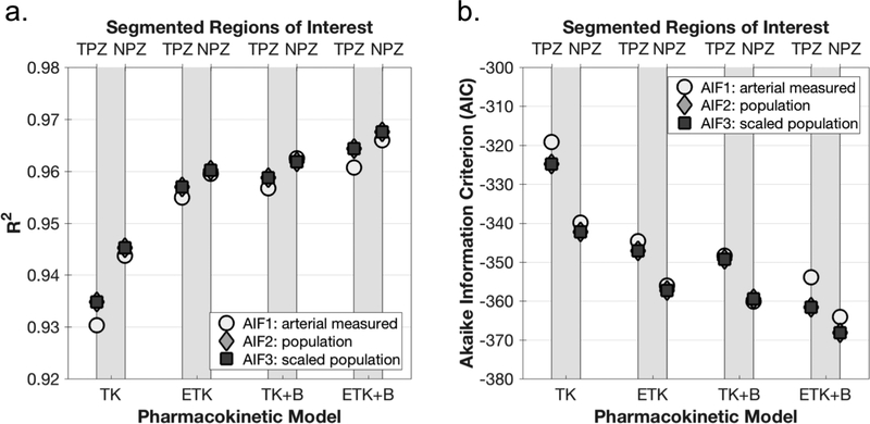
The model fits for a single representative voxel in the tumor-suspicious ROI of patient #7 is shown in Figure 4. Only the fits for AIF1 and AIF2 are shown, since the curves for AIF3 fall on top of those for AIF2. Generally, the more parameters are in the model, the less smooth is the resulting fitted curve. Figure 5 shows the mean Coefficient of Determination (R²) and Akaike Information Criterion (AIC) for the function fits in the 3 ROIs. Adding parameters to the model improves the fit in all ROIs, as expected. As shown, adding a 3rd parameter to the TK model (making it either ETK or TK+B) yields a larger improvement to the fit than adding a 4th parameter. Since the scaled population AIF fit values are practically indistinguishable from the unscaled population AIF values, it can be concluded that the goodness of fit is minimally affected by scaling the AIF.

Figure 5.

Comparison of Goodness of fit between analysis methods and regions of interest. Goodness of fit parameters were calculated for every voxel. Shown here is the mean (over patients and repeated scans) of the median goodness of fit parameter in each ROI. a. The coefficient of determination (R²). b. Akaike Information Criterion (AIC).

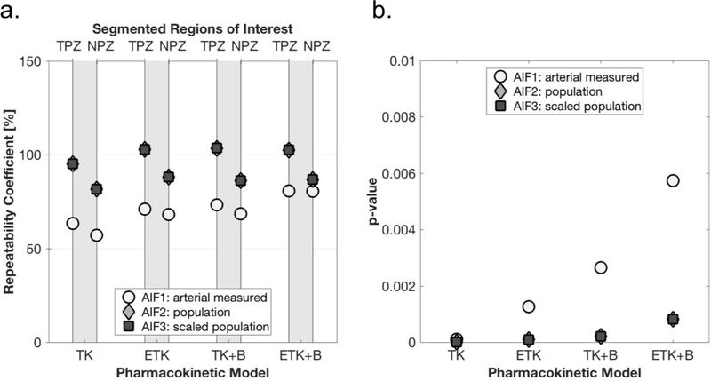
Due to relatively large differences in fitted parameter values between patients, %RC was deemed the more appropriate statistical measure to use for repeatability here.The %RC for parameter K_trans was generally lowest (indicating a more repeatable measurement) when using the scaled population AIF (AIF3), as shown in Figure 6a. The best repeatability for K_trans was achieved with the simplest model - the 2-parameter TK model, but the other models performed almost as well. Of the 3-parameter models (ETK and TK+B), repeatability was better with the addition of BAT fitting. The ROI with the most repeatable K_trans value was NPZ with a minimum of 59%, whereas the minimum %RC for TPZ was 83%. Discrimination between suspected pathological tissue in the TPZ ROI and normal peripheral zone tissue (NPZ ROI) according the p-values of the paired t-test was excellent, with p≤0.001 for all analysis methods and AIFs (Figure 6b).

Figure 6.

K_trans repeatability and tumor discrimination for different AIFs and analysis methods. a. %RC for AIFs (arterial, population, and scaled population) for the peripheral zone tumor-suspicious ROI (TPZ), and normal-appearing peripheral zone ROI (NPZ), for each analysis method. b. p-values from paired two-sided t-tests comparing K_trans in TPZ vs NPZ.

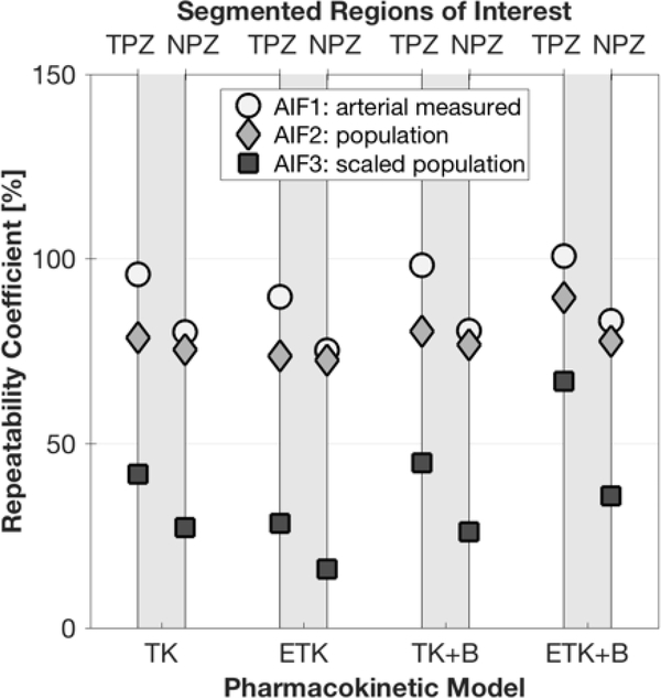
As illustrated in Figure 7, v_e was the most repeatable parameter as compared to K_trans and k_ep. %RC for v_e was always best in the case of the scaled population AIF (AIF3), with the ETK model yielding the most repeatable measurements - 16% for NPZ and 28% for TPZ (see Table 2 also). Addition of BAT fitting to the TK model did not significantly affect the repeatability of v_e, and BAT addition to the ETK model detracted from repeatability. Regarding differentiation between TPZ and NPZ - the paired t-test p-value was always above 0.1.

Figure 7.

v_e repeatability.

Table 2:

All values of parameter %RC and discrimination p-values, grouped according to pharmacokinetic model (TK, TK+BAT, ETK, ETK+BAT) and acording to AIF used (AIF1,AIF2,AIF3) showing the best value of %RC for each combination highlighted and in bold.

		Repeatability: %RC						Discrimination:
		TPZ ROI			NPZ ROI			p-value
		AIF1	AIF2	AIF3	AIF1	AIF2	AIF3	AIF1	AIF2	AIF3
Ktrans	TK	95%	93%	83%	78%	89%	59%	<10−4	<10−4	<10−4
	ETK	105%	119%	95%	94%	115%	84%	10−4	<10−4	<10−4
	TK+BAT	100%	102%	86%	80%	95%	67%	2·10−4	<10−4	<10−4
	ETK+BAT	130%	108%	93%	100%	101%	67%	10–3	7·10−4	4·10−4
ve	TK	96%	79%	42%	79%	76%	28%	0.60	0.84	0.81
	ETK	90%	74%	28%	75%	72%	17%	0.11	0.26	0.26
	TK+BAT	98%	80%	45%	80%	77%	26%	0.49	1	0.93
	ETK+BAT	101%	89%	67%	83%	78%	35%	0.36	0.89	0.94
kep	TK	63%	95%	95%	58%	83%	83%	10–4	<10−4	<10−4
	ETK	71%	103%	103%	68%	89%	89%	10–3	<10−4	<10−4
	TK+BAT	73%	103%	104%	69%	87%	87%	3·10−3	2·10−4	2·10−4
	ETK+BAT	81%	102%	103%	80%	86%	86%	5·10−3	7·10−4	7·10−4

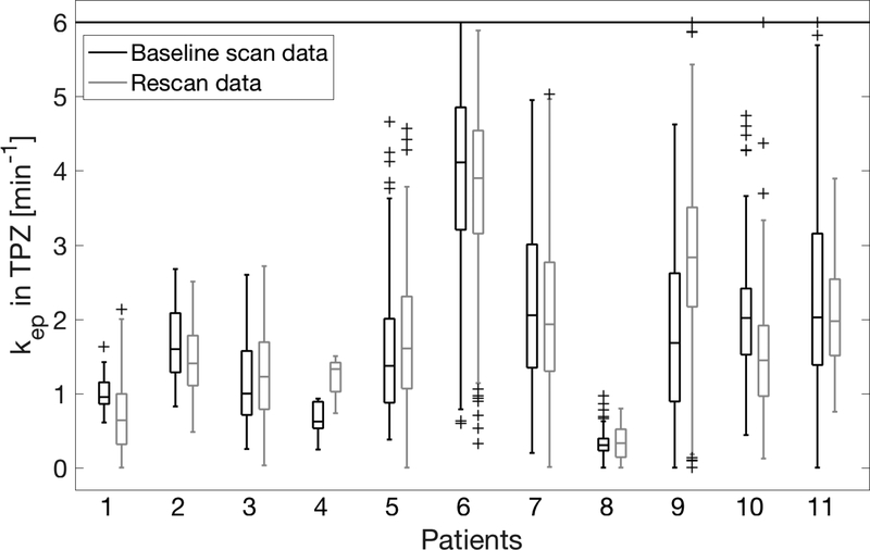
In the case of k_ep, the simplest model, TK, yielded the best repeatability, but not by much, as shown in Figure 8a. The minimum %RC was 57% for NPZ ROI and 63% for TPZ. Using a population AIF (or a scaled population AIF) as opposed to a measured arterial AIF, was not beneficial in the case of k_ep. To further illustrate the repeatability of k_ep, Figure 9 shows the distribution of k_ep values in the TPZ ROI of all patients and all scans. Differentiation of TPZ and NPZ was very good with p<0.006 for all models and AIF choices – see Figure 8b.

Figure 9.

Boxplots of calculated k_ep values in the tumor-suspicious region for all 11 patients. The two repeated scan results are shown next to each other for each patient, with a horizontal line at the median value and the box extent indicating the 25–75 percentiles. Values above 6 min⁻¹ are plotted at 6 min^-1.

Table 2 shows the values of repeatability and discrimination for all three parameters, with the optimal combination of pharmacokinetic model and AIF estimation method in bold.

Discussion

While prostate DCE analysis is generally challenging, it is important to determine the best methods for rendering clinical data usable for treatment response studies. In this study, the relative repeatability of extracted pharmacokinetic parameters using different analysis methods and AIF choices was assessed as an important characteristic of an imaging biomarker in order to help provide the groundwork to discriminate real change from measurement error. Since the relative repeatability of a parameter does not in itself justify its use as a biomarker - in addition to repeatability, each parameter was evaluated for its sensitivity to tissue pathological changes.

One of the conclusions from this study was that although a scaled population AIF (AIF3) was the best choice for K_trans repeatability and v_e repeatability, an arterial measured AIF (AIF1) was the best choice for k_ep repeatability. The result for k_ep makes sense in light of the AIF-scaling insensitivity of this parameter (suggested by its definition as K_trans/v_e) – this has been noted by others also (12). Although McGrath et al in their high temporal resolution study of DCE analysis on rat tumors using ETK, did not look at k_ep, they too found that repeatability and ICC for both K_trans and v_e was better with use of population average AIFs than with measured AIFs (9). In contrast, a DCE study of human liver found less scan-rescan variability when using a data-derived AIF than when using a model AIF (14). One must try to use a model AIF the functional form of which resembles the data AIFs (15), however it is unclear if this was not the case in (14).

Overall, in this study both K_trans and k_ep were excellent differentiators between tumor-suspicious tissue regions and normal-appearing regions in the prostate peripheral zone, as opposed to v_e that could not discriminate the two types of ROIs. Both K_trans and k_ep are widely recognised to be elevated in cancers - for a review, see Ref. (2).

Some of the limitations of this study include the small number of patients, the use of ROIs annotated by a single reader, and the absence of targeted biopsy procedures. However, the main objective here was to test parameter repeatability, independent of the exact pathological diagnosis. The lack of localized pathology confirmation of the disease presence in the TPZ ROIs may have contributed to higher minimum %RC values but this may not necessarily have affected the comparisons between models, AIFs and parameters.

We did not attempt to discriminate various sources that contribute to the variability of measurement beyond the DCE analysis parameters - these may have included imaging artifacts, gross motion of the patient and local motion due to peristalsis. While those aspects are important, their independent analysis was deemed not relevant here given the small size of the present dataset.

The simplest pharmacokinetic model, 2-parameter TK, performed best here in terms of parameter repeatability for parameters K_trans and k_ep. Other repeatability studies, performed in rodents, have not found differences between TK and ETK (29,30). Inclusion of a BAT term also did not improve repeatability, even with the use of unshifted population AIFs, and warrants further investigation. Other future plans include applying the improved understanding of the effect of analysis methods on particular DCE parameter repeatability as part of a response assessment study in patients that have undergone therapy in clinical trials conducted at our institution.

Abbreviations:

AIF

arterial input function

BAT

bolus arrival time

DCE

dynamic contrast-enhanced

ETK

extended Tofts-Kety

ETK+B

extended Tofts-Kety + BAT

NPZ

normal-appearing peripheral zone

PZ

peripheral zone

PI-RADS

Prostate Imaging – Reporting and Data System

PK

pharmacokinetic

RC

repeatability coefficient

%RC

percent repeatability coefficient

ROI

region of interest

TK

Tofts-Kety

TK+B

Tofts-Kety + BAT

TPZ

tumor-suspicious peripheral zone

References

- 1.Hara N, Okuizumi M, Koike H, Kawaguchi M, Bilim V. Dynamic contrast-enhanced magnetic resonance imaging (DCE-MRI) is a useful modality for the precise detection and staging of early prostate cancer. Prostate. 2005;62(2):140–147. [DOI] [PubMed] [Google Scholar]
- 2.Berman RM, Brown AM, Chang SD, et al. DCE MRI of prostate cancer. Abdom Radiol (NY). 2016;41(5):844–853. [DOI] [PMC free article] [PubMed] [Google Scholar]
- 3.Barrett T, Gill AB, Kataoka MY, et al. DCE and DW MRI in monitoring response to androgen deprivation therapy in patients with prostate cancer: a feasibility study. Magn Reson Med. 2012;67(3):778–785. [DOI] [PubMed] [Google Scholar]
- 4.Alic L, van Vliet M, van Dijke CF, Eggermont AMM, Veenland JF, Niessen WJ. Heterogeneity in DCE-MRI parametric maps: a biomarker for treatment response? Phys Med Biol. 2011;56(6):1601–1616. [DOI] [PubMed] [Google Scholar]
- 5.Kim H Variability in Quantitative DCE-MRI: Sources and Solutions. J Nat Sci. 2018;4(1):1–8. [PMC free article] [PubMed] [Google Scholar]
- 6.Heye T, Davenport MS, Horvath JJ, et al. Reproducibility of Dynamic Contrast-enhanced MR Imaging Part I. Perfusion Characteristics in the Female Pelvis by Using Multiple Computer-aided Diagnosis Perfusion Analysis Solutions. Radiology. 2013;266(3). doi: 10.1148/radiol.12120278/-/DC1 [DOI] [PubMed] [Google Scholar]
- 7.Sung YS, Park B, Choi Y, et al. Dynamic contrast-enhanced MRI for oncology drug development. J Magn Reson Imaging. 2016;44(2):251–264. [DOI] [PubMed] [Google Scholar]
- 8.Fedorov A, Fluckiger J, Ayers GD, et al. A comparison of two methods for estimating DCE-MRI parameters via individual and cohort based AIFs in prostate cancer: a step towards practical implementation. Magn Reson Imaging. 2014;32(4):321–329. [DOI] [PMC free article] [PubMed] [Google Scholar]
- 9.McGrath DM, Bradley DP, Tessier JL, et al. Comparison of mode-based arterial input functions for dynamic contrast-enhanced MRI in tumor bearing rats. Magn Reson Med 2009; 61:1173–1184. [DOI] [PubMed] [Google Scholar]
- 10.Lu H, Clingman C, Golay X, van Zijl PCM. Determining the longitudinal relaxation time (T1) of blood at 3.0 Tesla. Magn Reson Med. 2004;52(3):679–682. [DOI] [PubMed] [Google Scholar]
- 11.Sourbron SP, Buckley DL. Classic models for dynamic contrast-enhanced MRI. NMR Biomed. 2013;26(8):1004–1027. [DOI] [PubMed] [Google Scholar]
- 12.Li X, Cai Y, Moloney B, et al. Relative sensitivities of DCE-MRI pharmacokinetic parameters to arterial input function (AIF) scaling. J Magn Reson. 2016;269:104–112. [DOI] [PMC free article] [PubMed] [Google Scholar]
- 13.Keil VC, Maedler B, Gieseke J, et al. Effects of arterial input function selection on kinetic parameters in brain dynamic contrast-enhanced MRI. Magn Reson Imag. 2017; 40:83–90. [DOI] [PubMed] [Google Scholar]
- 14.Ashton E, Raunig D, Ng C, Kelcz F, McShane T, Evelhoch J. Scan-rescan variability in perfusion assessment of tumors in MRI using both model and data-derived arterial input functions. J Magn Reson Imaging. 2008;28(3):791–796. [DOI] [PubMed] [Google Scholar]
- 15.Azahaf M, Haberley M, Betrouni N, et al. Impact of arterial input function selection on the accuracy of dynamic contrast-enhanced MRI quantitative analysis for the diagnosis of clinically significant prostate cancer. 2016; JMRI 43(3):737–749. [DOI] [PubMed] [Google Scholar]
- 16.Huang W, Chen Y, Fedorov A, et al. The Impact of Arterial Input Function Determination Variations on Prostate Dynamic Contrast-Enhanced Magnetic Resonance Imaging Pharmacokinetic Modeling: A Multicenter Data Analysis Challenge. Tomography. 2016;2(1):56–66. [DOI] [PMC free article] [PubMed] [Google Scholar]
- 17.Mehrtash A, Gupta SN, Shanbhag D, et al. Bolus arrival time and its effect on tissue characterization with dynamic contrast-enhanced magnetic resonance imaging. J Med Imaging (Bellingham). 2016;3(1):014503. [DOI] [PMC free article] [PubMed] [Google Scholar]
- 18.Chouhan MD, Bainbridge A, Atkinson D, et al. Estimation of contrast agent bolus arrival delays for improved reproducibility of liver DCE MRI. Phys Med Biol. 2016;61(19):6905–6918. [DOI] [PMC free article] [PubMed] [Google Scholar]
- 19.Fedorov A, Vangel MG, Tempany CM, Fennessy FM. Multiparametric Magnetic Resonance Imaging of the Prostate: Repeatability of Volume and Apparent Diffusion Coefficient Quantification. Invest Radiol. 2017;52(9):538–546. [DOI] [PMC free article] [PubMed] [Google Scholar]
- 20.Weinreb JC, Barentsz JO, Choyke PL, et al. PI-RADS Prostate Imaging - Reporting and Data System: 2015, Version 2. Eur Urol. 2016;69(1):16–40. [DOI] [PMC free article] [PubMed] [Google Scholar]
- 21.Fennessy FM, Fedorov A, Gupta SN, Schmidt EJ, Tempany CM, Mulkern RV. Practical considerations in T1 mapping of prostate for dynamic contrast enhancement pharmacokinetic analyses. Magn Reson Imaging. 2012;30(9):12241233. [DOI] [PMC free article] [PubMed] [Google Scholar]
- 22.Tofts PS, Kermode AG. Measurement of the blood-brain barrier permeability and leakage space using dynamic MR imaging. 1. Fundamental concepts. Magn Reson Med. 1991;17(2):357–367. [DOI] [PubMed] [Google Scholar]
- 23.Parker GJM, Roberts C, Macdonald A, et al. Experimentally-derived functional form for a population-averaged high-temporal-resolution arterial input function for dynamic contrast-enhanced MRI. Magn Reson Med. 2006;56:993–1000. [DOI] [PubMed] [Google Scholar]
- 24.Kety SS. The theory and applications of the exchange of inert gas at the lungs and tissues. Pharmacol Rev. 1951;3(1):1–41. [PubMed] [Google Scholar]
- 25.Tofts PS, Brix G, Buckley DL, et al. Estimating kinetic parameters from dynamic contrast-enhanced T(1)-weighted MRI of a diffusable tracer: standardized quantities and symbols. J Magn Reson Imaging. 1999;10(3):223–232. [DOI] [PubMed] [Google Scholar]
- 26.Akaike H A new look at the statistical model identification. IEEE transactions on automatic control. 1974; AC-19(6):716–723. [Google Scholar]
- 27.Bland JM, Altman DG. Measurement Error. British Medical Journal. 1996;312:1654. [DOI] [PMC free article] [PubMed] [Google Scholar]
- 28.Obuchowski NA. Interpreting Change in Quantitative Imaging Biomarkers. Acad Radiol. 2018;25(3):372–379. [DOI] [PMC free article] [PubMed] [Google Scholar]
- 29.Ng CS, Wei W, Bankson JA, et al. Dependence of DCE-MRI biomarker values on analysis algorithm. 2015; PLoS One 10(7): e0130168. [DOI] [PMC free article] [PubMed] [Google Scholar]
- 30.Barnes SL, Whisenant JG, Loveless ME, Ayers GD and Yankeelov TE. Assessing the reproducibility of dynamic contrast enhanced magnetic resonance imaging in a murine model of breast cancer. Magn Reson Med 2013; 69:1721–1734. [DOI] [PMC free article] [PubMed] [Google Scholar]