Optimal decoding of cellular identities in a genetic network

Summary

In developing organisms, spatially prescribed cell identities are thought to be determined by the expression levels of multiple genes. Quantitative tests of this idea, however, require a theoretical framework capable of exposing the rules and precision of cell specification over developmental time. Using the gap gene network in the early fly embryo as an example, we use such a framework to show how expression levels of the four gap genes can be jointly decoded into an optimal specification of position with 1% accuracy. The decoder correctly predicts, with no free parameters, the dynamics of pair-rule expression patterns at different developmental time points and in various mutant backgrounds. Precise cellular identities are thus available at the earliest stages of development, contrasting the prevailing view of positional information being slowly refined across successive layers of the patterning network. Our results suggest that developmental enhancers closely approximate a mathematically optimal decoding strategy.

Graphical Abstract

In brief:

The information to specify precise cellular identities is present and decoded at the earliest stages of Drosophila development, contrasting with the view that positional information is slowly refined across successive patterning layers.

Introduction

Biological networks transform input signals into outputs that capture information of functional importance to the organism. One path to understanding these transformations is to “read out,” or decode this relevant information directly from the network activity (Georgopoulos et al., 1986; Haynes and Rees, 2006). In neural networks, for example, features of the organism’s sensory inputs and motor outputs have been decoded from observed action potential sequences, sometimes with very high accuracy (Hatsopoulos and Donoghue, 2009; Marre et al., 2015; Rieke et al., 1997). Decoding provides an explicit test of hypotheses about how biologically meaningful information is represented in the network.

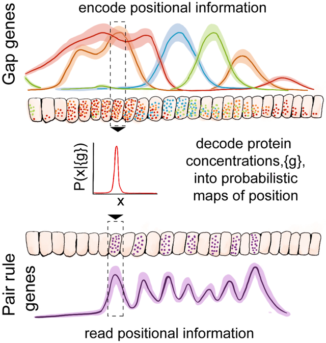
The gap genes involved in patterning the early embryo of the fruit fly Drosophila melanogaster provide an alternative example of the decoding problem (Briscoe and Small, 2015; Jaeger, 2011; Nüsslein-Volhard and Wieschaus, 1980). Individually, the gap genes form a network with strong, bidirectional couplings among themselves. But, taken together, the gap genes form a single layer in an otherwise feed-forward flow of information, where they take inputs from the primary maternal morphogens and drive the expression of pair-rule genes (Carroll, 1990; Rivera-Pomar and Jäckle, 1996) (Figure 1A). Pair-rule expression occurs in stripes that are precisely and reproducibly positioned within the embryo, forming an outline for the segmented body plan of the fully developed organism (Lawrence, 1992).

Figure 1: Decoding in a genetic network.

(A) In the early Drosophila embryo, maternally provided morphogens (bcd, nos, tor) regulate the expression of gap genes (kni, kr, gt, hb), which is visualized here in a mid-sagittal slice through an embryo during n.c. 14 (scale bars, 100 μm). Enhancers (schematically depicted as circles) respond to combinations of gap protein concentrations to drive pair-rule gene expression that occurs in a precise and reproducible striped pattern (Gregor et al., 2014). (B) Schematic depiction of the decoding problem. Positional information is supplied by three morphogens primarily acting in the anterior A, posterior P, or terminal T domains. The network can be viewed as an input/output device that encodes physical location x in the embryo using concentrations {g₁, g₂, g₃, g₄} of the gap gene proteins. Optimal decoding is a well-posed mathematical problem, whose solution is found in the posterior distribution P(x*∣{g_i}) (Equation 3); results can be visualized as a decoding map, P(x*∣x) (Equation 4 and Figure 2). The posterior distribution is constructed from measurements (average gap gene expressions, $\{{\stackrel{‒}{g}}_i(x)\}$ and their covariability, C_ij(x), and contains no arbitrary parameters. (C) Testable predictions from optimal decoding. Pair-rule stripes are expected wherever decoding a combination of concentrations yields an implied position, X*, associated with a pair-rule stripe, $X_{\text{str}}^{\ast }$, in WT.

The emergence of a precise and reproducible body plan requires each cell in the developing embryo to take actions that are appropriate to its position. Previous work has shown that a snapshot of gap gene expression levels contains enough information to position each cell with ~ 1% precision along the embryo’s anterior-posterior (AP) axis (Dubuis et al., 2013a; Tkačik et al., 2015). This is comparable to the precision with which pair-rule patterns and other morphological markers are specified. The fact that this information is available, however, does not mean that it is used by the organism. Here we take the pair-rule stripes as a measure of the embryo’s own readout of positional information, and test this idea explicitly: we decode the positional information conveyed by gap gene expression levels, and use this decoder to predict the dynamics of pair-rule stripes in wild-type (WT) and their distortions in mutant embryos (Figure 1).

We can imagine many different ways of decoding gene expression levels to estimate position, but there is a unique optimal decoding scheme. More specifically, if the embryo makes use of all the available information then the statistical structure of gap gene expression patterns determines the form of the decoding algorithm (Figure 1B), without the need for an explicit model or for any additional parameters; decoded positions then predict the occurrence of pair-rule stripes (Figure 1C). To construct the optimal decoder, we measured all gap gene expression levels simultaneously and with sufficient accuracy to characterize the noise in the system. This allows us to give a good description of the joint distribution of gap gene expression levels at each position along the AP axis, and these distributions in turn determine the form of the optimal decoder.

To test the optimal decoder, we employ seven distinct genetic variants that alter primary maternal inputs. We show that a single optimal decoder constructed from WT data accounts, quantitatively, for the altered locations of pair-rule stripes in mutant embryos, for the dynamical shifts of the pair-rule stripes in WT embryos, and even predicts when the occurrence of these stripes should be variable. These results fit into a broader picture of early embryonic patterning in Drosophila as a system in which 1) noise levels are as low as possible given the limited number of molecules involved (Gregor et al., 2007), 2) the reproducibility of developmental patterning can be traced back to reproducible maternal inputs (Petkova et al., 2014), and 3) network interactions are selected to extract the maximum amount of information from these inputs (Sokolowski and Tkačik, 2015; Tkačik et al., 2008, 2012; Walczak et al., 2010). Stated in more mechanistic terms, our results suggest that the complex regulatory logic of the pair-rule gene enhancers (Levine, 2010; Small et al., 1991) implements nearly optimal decoding of gap gene network activity, and thus provides access to precise and potentially unique cellular identities already at the earliest stages of development; i.e. four genes are sufficient to uniquely predict the fates of ~60 cells along the central 80% of the dorsal line in the early fly embryo (Dubuis et al., 2013a).

Results

Dictionaries, maps, and optimality

There is a clear advantage to organisms that can construct a rich and precise body plan, specifying the detailed pattern of structures at different positions. It is less clear when this positional information needs to be available, or whether evolutionary pressures have been strong enough to drive mechanisms that extract as much positional information as possible given the physical constraints. Here we test the hypothesis that the fly embryo achieves an optimal decoding of position given access to the gap gene expression levels in each individual nucleus, at a single moment in time. While optimality is a controversial hypothesis (Bialek, 2012), we emphasize that, in the present context, it makes unambiguous, quantitative predictions, which we test.

Let {g_i} = {g₁, g₂, g₃, 9₄} be the expression levels of the gap genes hunchback (hb), krüppel (Kr), knirps (kni), and giant (gt). At each point x along the embryo’s AP axis, gap gene expression levels take on average values, ${\overline{g}}_{\mathrm{i}}(x)$, but also exhibit fluctuations around this mean that can be summarized with a 4×4 covariance matrix, C_ij(x). Exploiting our ability to make precise, quantitative measurements of the expression of all four gap genes simultaneously across many embryos (Dubuis et al., 2013b), we construct $\{{\overline{g}}_{\mathrm{i}}(x)\}$ and C_ij(x) (Star Methods and Figures S1A and S1B), initially focusing on a small time window, centered 42 min into nuclear cycle (n.c.) 14, in which mutual information about position carried by the gap gene expression profiles is highest (Dubuis et al., 2013a).

If the fluctuations are Gaussian (an approximation tested previously (Dubuis et al., 2013a)), then the mean expression level and the covariance matrix determine the joint probability distribution of gap gene expression levels given position. Explicitly, for the simultaneous expression levels of K genes:

$$P(\{g_i\}\mid x)=\frac{1}{\sqrt{(2\pi {)}^K\text{det}[\widehat{C}(x)]}}{e}^{-{\chi }_K^2(\{g_i\},x)∕2},$$ (1)

where ${\chi }_K^2$ measures the similarity of the gene expression pattern to the mean pattern $\{{\overline{g}}_{\mathrm{i}}(x)\}$ expected at x,

$${\chi }_K^2(\{g_{\mathrm{i}}\},x)=\sum _{\text{i,j}=1}^K(g_{\mathrm{i}}-{\overline{g}}_{\mathrm{i}}(x)){\left({\widehat{C}}^{-1}(x)\right)}_{\text{ij}}\left(g_{\mathrm{j}}-{\overline{g}}_{\mathrm{j}}(x)\right),$$ (2)

and $\widehat{C}(x)$ is the covariance matrix. We previously estimated the information that individual gap gene expression levels provide about position assuming only that the underlying probability distribution is smooth, and this agrees within error bars with the information calculated in the Gaussian approximation (Dubuis et al., 2013a; Tkačik et al., 2015). Thus this approximation is not a model of the system, but a compact summary of its behavior that captures the relevant information. From this summary, and the hypothesis of optimality, we will make predictions for the results of very different measurements, with no additional parameters that need to be fit.

To construct the optimal decoder, we apply Bayes’ rule (Star Methods):

$$P(x^{\ast }\mid \{g_{\mathrm{i}}\})=\frac{1}{Z(\{g_{\mathrm{i}}\})}P(\{g_{\mathrm{i}}\}\mid x^{\ast })P_X(x^{\ast }),$$ (3)

where the left-hand side, called the posterior, is a distribution over positions x* that are implied by some combination of gap gene expression levels {g_i}. Implied because the decoder has no access to the actual position of a cell; it can only use the four gap gene expression levels {g_i}, which provide varying amounts of evidence for different possible positions. P_X(x*) is the (prior) probability that a cell is at position x*, independent of gene expression level, and is in our case uniform along the AP axis; Z serves to normalize the distribution, and is independent of x*.

The posterior P(x*∣{g_i}) contains all the information that any mechanism, cellular or computational, could extract from expression levels {g_i}. If the posterior has a single, reasonably sharp peak at x* = X*({g_i}), then we can translate expression levels back into positions unambiguously, using a dictionary {g_i} → X*; this is known as the maximum a posteriori (MAP) decoder (David J. C. MacKay, 2003). The width of the distribution P(x*∣{g_i}) around its peak quantifies the positional error, i.e., the uncertainty in implied position due to the variability in gap gene expression levels (Tkačik et al., 2015). But if the posterior has multiple peaks, or broad plateaus, then genuine ambiguities in decoding exist and the MAP decoder is misleading. We keep track of the entire posterior distribution of implied positions and visualize it as a decoding map (Figure 2).

Figure 2: Coding and decoding of position in fly embryos.

(A) Optical section through the midsagittal plane of a Drosophila embryo with immunofluorescence labelling for Krüppel (Kr) protein (scale bar, 100μm). Raw dorsal fluorescence intensity profile of depicted embryo (blue curve, gα(x)) and encoding probability distribution P(Kr∣x) (gray) constructed from 38 WT embryos of ages between 40–44 min into n.c. 14. Position x along the AP axis is normalized by embryo length L, with x/L = 0 (1) for the anterior (posterior) poles. Probability distribution of Kr expression levels (left). (B) Decoding probability distribution P(x∣Kr) constructed via Bayes’ rule from the measured probability distributions P(g) and P(g∣x) in (A), using a uniform prior P_X(x) = 1/L. P(x∣Kr) is input for the optimal decoder, which maps Kr levels to positions along the AP axis. Posterior probability distributions of locations x consistent with observing Kr levels 0.05, 0.5, or 1 are the conditional probability densities P(x∣Kr) shown in top panels. (C) Decoding map $P_g^{\alpha }(x^{\ast }\mid x)$ for a single embryo α. Top cartoons display regions of inferred positions based on Kr alone. Dynamic range (gray bar, right) applies to all three probability panels. See also Figure S1.

To construct the decoding map for a single embryo α, we take the measured expression levels $\{g_{\mathrm{i}}^{\alpha }(x)\}$ in that embryo at actual position x and insert them into Equation (3). This yields a map of implied positions vs actual positions,

$$P_{\text{map}}^{\alpha }(x^{\ast }\mid x)=P(x\mid \{g_{\mathrm{i}}\}){\mid }_{\{g_{\mathrm{i}}\}=\{g_{\mathrm{i}}^{\alpha }(x)\}}.$$ (4)

If the considered genes provide enough information to specify position accurately and unambiguously, then $P_{\text{map}}^{\alpha }(x^{\ast }\mid x)$ will be a narrow ridge of density along the diagonal where the implied position is equal to the actual position, x* = x. Figure 2 walks through the steps in the construction of the decoding map $P_{\text{map}}^{\alpha }(x^{\ast }\mid x)$ in the case where we have access to the expression level of only one gene, in this case Kr.

Using a data set of 38 WT embryos, we construct decoding maps based on the information carried by one, two, three, or all four gap genes (Figure 3). Note that although we always decode the gene expression levels from single embryos, as in Equation (4), it is convenient to show maps that are averaged over all the embryos α in our data. For most locations in the embryo, decoding based on a single gene provides little information (Figures 2 and 3a and S1c). In small regions of the embryo, decoding can be more precise, but substantial ambiguities remain where one expression level is equally consistent with two different implied positions. Decoding based on two (Figures 3B and S1D) or three (Figures 3C and S1E) genes results in less ambiguity and more precision.

Figure 3: Decoding with increasing number of gap genes in WT embryos.

Top row: dorsal fluorescence intensity profile(s) from simultaneously stained embryos (mean ± SD); units scaled so that 0 (1) corresponds to minimum (maximum) mean expression. Bottom row: decoding maps, P(x*∣x) from Equation (4), averaged over 38 embryos. (A) Decoding using single gene (Kr, blue) (also Figures 2 and S1C). (B) Decoding using a combination of two genes, Kr (blue) and Hb (red) (also Figure S1D). (C) Decoding using three genes, Kr (blue), Hb (red), and Gt (orange) (also Figure S1E). (D) Decoding using all four gap genes. See also Figure S1.

We report the decoding maps in units of probability density, because the x coordinate is treated as continuous, which lets us construct mathematical objects independent of the choice of binning scheme for positions. The increase in precision corresponds to the sharpening of the posterior distribution, whose peaks get higher and narrower as we include increasing numbers of gap genes. This increase is reflected in the dynamic range of grayscales for each map, since by normalization narrower distributions $P_{\text{map}}^{\alpha }(x^{\ast }\mid x)$ have higher density at their peaks. We also quantify this sharpening by computing the standard deviation of these distributions and finding the median over x as summarized in Figure S1I.

With all four genes, the distribution $P_{\text{map}}^{\alpha }(x^{\ast }\mid x)$ is approximately Gaussian, with a width σ_x ~ 0.01L for nearly all points along the embryo’s AP-axis (Figures 3D and S5A). This is also the precision with which subsequent developmental markers, including the pair-rule gene stripes and the cephalic furrow, are generated (Dubuis et al., 2013a; Liu et al., 2013). Remarkably, one percent is less than the distance between two adjacent cells, suggesting that the gap genes could specify every cell along the AP-axis (Dubuis et al., 2013b, 2013a). Thus multiple expression levels combine to synthesize an unambiguous code for position that reaches extraordinary precision (Figure 3).

We emphasize that we decode positions based on graded expression levels of the gap genes (Dubuis et al., 2013a; Gaul and Jackle, 1989), which contrasts with the traditional interpretation of the gap genes as forming “expression domains” that are either on or off (Albert and Othmer, 2003; B Alberts, A Johnson, J Lewis, M Raff, K Roberts, 2002; Meinhardt, 1986), or with the use of binary switch-like or boolean networks to describe genetic circuits more generally (Kauffman et al., 1978; Sánchez and Thieffry, 2001). If we collapse the continuous profiles into on/off domains, then decoding maps are ambiguous even in WT embryos (Figures S1F and S1G), and meaningful predictions for stripe positions in the mutant embryos are impossible. Thus, rather than forming a set of four binary switches, the gap gene expression levels represent a more continuous, analog coordinate system that specifies position for individual cells.

Decoding in mutant embryos

The fact that the four gap genes carry precise, unambiguous information about position does not mean that the embryo uses this information to determine cellular identities. To test whether this is the case, we exploit the powerful genetic tools that have been established in Drosophila. We perturbed the maternal signals Bicoid (bcd), Nanos (nos), and Torso-like (tsl), which strongly affect the gap gene network (Figure S2 and Movie M1). Importantly, because we have perturbed only the inputs to the gap gene network, we expect that decoding is carried out with the same mechanism in WT and mutant embryos. If the optimal readout strategy is used by the embryo, our decoder should generate meaningful position estimates in mutant backgrounds (Equation 4), and these estimates can be compared directly to actual position readouts in mutant embryos, using locations of pair-rule expression stripes as positional markers.

We have analyzed embryos from lines in which we delete the three maternal signals individually, in pairs, and all together. The latter is a control, which confirms that all information about position indeed is provided by the three maternal signals (Figure S2K). For each of the remaining six combinations, we measured expression levels for all four gap genes simultaneously (Figure S2A-H). In every case, we construct the posterior distribution P(x*∣{g_i}) from WT gene expression levels in absolute units, and then apply it to individual mutant embryos measured in the same batch, thus avoiding variations in staining, imaging, normalization, etc., across batches. The results of these analyses are a series of decoding maps (Figure 4), which should be compared to the map for WT embryos (Figure 3D).

Figure 4: Decoding maps and stripe locations in mutant embryos.

Average decoding maps for six maternal mutant backgrounds (whitened APT symbols above the panels signify whether the anterior A, posterior P, or terminal T systems are deficient): (A) etsl⁴; (B) bcd^E1; (C) osk¹⁶⁶; (D) bcd^E2 osk¹⁶⁶; (E) Bcd-only germline clone; (F) bcd^E etsl¹; same gray-scale as in Figure 3D. Measured Eve expression profiles in WT embryos (left side of A and D), and in mutant embryos (below each corresponding decoding map); individual profiles (gray), mean profile (black), and peak locations (black dots), units scaled so that 0 (1) corresponds to minimum (maximum) mean Eve expression within each genotype. Average locations of WT Eve stripes (horizontal dotted lines) are used to predict Eve stripes in the mutant backgrounds: stripes expected at AP locations in mutant embryos where horizontal dotted lines intersect peak(s) of the probability density. Open black circles mark intersections of horizontal dotted lines and respective average locations of Eve stripes in mutant embryos (vertical dotted lines). Variable number of Eve stripes highlighted by horizontal starred bars (see B and F; see Figure S6). Red line in C marks observed Eve stripe that is not predicted by the decoding map. Red line in E shows a predicted Eve stripe that is not observed in the mutant embryo. When horizontal lines intersect a broad probability distribution, we expect to observe diffuse Eve stripes as in F. A shows additional predictions for Run (cyan) and Prd (magenta) stripes; the dense collection of markers traces the ridge of implied positions in the decoding map with very high accuracy. See also Figures S2, S3, and S4 and Movie M1.

Before proceeding to analyze these maps and to test our predictions, we emphasize that even the possibility of decoding the expression patterns in mutant backgrounds is non-trivial. The optimal decoder is built out of the distribution of expression levels that we see in WT embryos, and these fill only a very small region of the full four dimensional space of possibilities. If the expression levels in mutant embryos fell far outside this region, then we would have no reason to trust our description of the distributions P({g_i}∣x), and hence no basis from which to make reliable inferences. To test whether this could be the case, we compared χ² in Equation (2) between the mean WT and the mutant gap gene expression (see Star Methods, Exploring mutant embryos). We found a surprising degree of overlap: the largest χ² in the WT embryos is larger than 98% of the values that we see in mutant embryos (Figure S2I); extreme values of χ² in the mutant backgrounds are confined to small regions of the embryo. Deleting maternal signals introduces large perturbations, yet the gap gene network responds in a way that is not far outside the distribution of possible responses under WT conditions. This fact is what makes decoding positional information in mutant embryos feasible.

Many features of the decoding maps in Figure 4 are expected from previous, qualitative characterizations of these mutant backgrounds. Thus, when we delete tsl the distortions are largely at the embryo’s poles (Figure 4A), to which tsl expression is confined (Martin et al., 1994); and when we delete osk (which controls the localization of the nos signal), we see major distortions in the posterior (Figure 4C), consistent with nos being a posterior determinant (Wang and Lehmann, 1991). When we delete bcd there are major distortions in the anterior portion of the map (Figure 4B), where the concentration of Bcd protein is highest, but distortions of the map extend along the entire length of the embryo, in contrast to the more local effects of removing tsl or nos.

To further characterize the maternal patterning inputs, we examined double mutant backgrounds, in which the positional information is supplied by a single remaining maternal input (Figures 4D-F). When the only spatial information is supplied by tsl or nos (in embryos from mothers doubly mutant for bcd nos or bcd tsl, respectively), the resultant embryos lack much of the WT gap gene pattern. Inferred positions based on the levels of the remaining gap genes at no point match the diagonal defined by the WT pattern.

One challenge in analyzing embryos with patterning information only from Bcd is that removal of nos and tsl results in uniformly high ectopic levels of maternal Hb (Hulskamp et al., 1989; Struhl, 1989). These uniform levels confer no positional information but the repressive activity of Hb as a transcription factor blocks expression of gap genes and thus all patterning in the abdomen (Gavis et al., 2008; Irish et al., 1989). As an alternative, we have generated germline clones (Hannon et al., 2017), which lack maternal hb activity, as well as positional cues from nos and tsl. These mutant backgrounds have a rich collection of pair-rule stripes, providing a more detailed test of our theory. Surprisingly, decoding maps in these mutant embryos (Figure 4E) have a nearly continuous ridge of density, with a width close to that in WT, that runs nearly from x/L = 0.3 to x/L = 0.8. This is qualitatively consistent with the observation that these embryos show WT patterns between the gnathal and 6th abdominal segments (Hannon et al., 2017). It is also surprising that we can achieve precise (if distorted) decoding at x/L ~ 0.8, where the only source of positional information is the Bcd protein, which is present at very low concentrations (Little et al., 2011 and 2013).

Testing the dictionary, quantitatively

While the predictions of optimal decoding are in qualitative agreement with expectations from previous work, it is crucial that this theoretical framework makes detailed quantitative predictions about positions. The peaks of pair-rule expression are positional markers that predict features of the final body plan, and thus we take these peaks as a measure of the embryo’s own readout of positional information (Figure S5B–D). Independent of our work, it is much less clear how levels of pair-rule expression relate to development; therefore, the units of pair-rule gene expression are normalized within each genotype, and we make no attempt to compare these levels across genotypes.

As a first example, when we delete bcd (Figure 4B), quantitative distortions of the map extend even into the posterior half of the embryo, so that the map is shifted, and the plot of x* vs x (following the ridge of high probability in the map) does not have unit slope. In particular, expression levels found at x/L = 0.7 (or at x/L = 0.55) have their most likely decoded values at x*/L = 0.75 (or x*/L = 0.67). But in the WT embryo, positions x/L = 0.75 and x/L = 0.67 are associated with the stripes vii and vi of expression for the pair-rule gene eve, as shown at left in Figure 4. If the machinery for interpreting gap gene expression is using the same dictionary that we have constructed mathematically, then we predict that the bcd deletion mutants should shift these two eve stripes to x/L = 0.7 and x/L = 0.55, which is what we see (Figure 4B). More dramatically, expression levels at x/L = 0.23 in the bcd mutant background are decoded as x*/L = 0.75 with high probability, and correspondingly there is an eve expression pattern at this anomalously anterior location. This is predicted to be not a displacement of the first (nearest) eve stripe, but rather a duplication of the seventh stripe, which is consistent with classical observations on cuticle morphology in these mutant backgrounds (Driever and Nüsslein-Volhard, 1988), and with recent RNAi/reporter experiments (Staller et al., 2015).

The quantitative agreement between the decoding maps and the locations of the eve stripes extends to all six examples of single and double maternal mutants shown in Figure 4, as well as to the prediction of stripe locations for the pair-rule genes paired (prd) and runt (run) (Figures S3 and S4). Notably, there is good agreement both when the shifts are small, as with the deletion of tsl (Figure 4A), and when the shifts are much larger, resulting in the deletion of several stripes, as with the bcd osk and bcd tsl double mutants (Figures 4D and 4F). In cases where the implied position of a stripe crosses a diffuse band of probability density in the decoding map, as in the anterior of the bcd tsl mutant, we might expect that there would be expression of eve but not a sharp stripe, and this is what we see (Figure 4F).

For simplicity Figure 4 shows decoding maps that are averaged over all embryos for each mutant line. If we focus instead on decoding maps for individual embryos, their variability predicts the embryo-to-embryo variability in pair-rule gene expression. In particular, for bcd tsl mutants the positions that map to the WT locations of eve stripes iv and v (x*/L = 0.56 and x*/L = 0.62) vary substantially in the window 0.4 < x/L < 0.6. If we look at the eve expression patterns in individual embryos (thin lines at bottom of Figure 4F; for detailed analysis see Figure S6A-C), we see two peaks with variable positions, as predicted. For the bcd mutant, the average decoding map again has density at x*/L = 0.56 and x*/L = 0.62 (Figures 4B and S6D-F), but when we decode the gap gene expression patterns from individual mutant embryos we find that these features vary not only in their position but even in their presence or absence, so that individual embryos are predicted to have a variable number of eve stripes, and this is again what we see.

There are a small number of errors in our predictions. In the osk mutants a posterior Eve stripe is observed where none is predicted (Figure 4C), and in bcd osk mutants we predict a variable number of Prd stripes (Figure S3D). A Run stripe is predicted at x/L ~ 0.6 where none is observed (Figure S4C); and we have no prediction for the very blurred band of Run expression at x/L > 0.7 (Figure S4C). In addition, in the bcd tsl mutant a Run stripe is predicted at x/L ~ 0.45 where none is observed (Figure S4F). Another failure occurs at a rare point where the combinations of gap gene expression are outside the range sampled in the WT embryos (Figure S2J), and thus we may be simply extrapolating the probability distributions too far.

In the WT embryo, local decoding of gap gene expression levels always leads to smooth maps, so that spatial averaging would not result in any systematic changes. Further, fluctuations in the expression level are correlated over significant distances (Krotov et al., 2014), so that spatial averaging also would not reduce the noise or enhance the reliability of decoded positions. These arguments fail at a small number of locations in the mutants where the decoding map has a dramatic discontinuity, as in the osk mutants (Figure 4C). In this case, any spatial averaging would involve combining vastly different signals, and the outcome would depend on the details of the averaging process, so we lose predictive power based on the maps alone.

Finally, a more quantitative survey compares how well the predictions of pair-rule stripe positions based on the decoding maps correspond to the actual measured positions in the six mutants for all eve, run, and prd stripes (Figure 5). For nearly all of the 70 identifiable pair-rule stripes, the predicted position agrees with the measured position within the measured embryo-to-embryo variability. Further, direct comparison of the horizontal and vertical error bars in Figure 5 reveals that also the measured variability in stripe positions is in good agreement with the predicted variability (Figure S6G), again a highly nontrivial connection between the decoding map and embryo-to-embryo fluctuations in mutant gap gene expression. This rich and tight correspondence between measurements and predictions for stripe positions (and even their variability) implies that developmental enhancers in the Drosophila embryo implement a close analogue of the mathematically optimal decoding scheme, efficiently reading out gap gene expression levels and transforming them into a positional specification with 1% accuracy, sufficient for precise assignment of cellular identities along the AP axis.

Figure 5: Predicted vs observed locations of 70 pair-rule stripes in mutant embryos.

Horizontal axis: measured pair-rule stripe positions in mutant embryos (mean ± SD across embryos of a given genotype). Vertical axis: predictions from decoding the gap gene expression levels in mutant embryos (mean ± SD across embryos of a given genotype). Color scale indicates the displacement of the observed peak from its WT location (Δx/L). 11 diffuse stripes are analyzed separately (Figure S5). In addition, we observe, but do not predict 3 stripes; and predict, but do not observe 3 stripes. See also Figures S5 and S6.

Dynamics in wild-type embryos

Gap gene expression levels vary in time, even within n.c. 14 (Jaeger, 2011). In principle we could ask about the information contained in these expression levels, moment by moment, allowing for the possibility that the best decoding of this information also varies in time. If, on the other hand, we imagine that the embryo implements a single decoder, optimized—as in the discussion above—to extract maximum positional information at the moment when this information itself is maximal (Dubuis et al., 2013b, 2013a), then we necessarily predict that the map of implied vs actual position will change over time. Thus, following the same logic as in our analysis of mutants, the stripes of pair-rule gene expression should shift over time, which is known to happen. The question is whether our optimal decoder predicts the correct quantitative pattern of stripe dynamics.

The possibility of using dynamics as a test of optimal decoding hinges on our ability to stage the developmental time of fixed embryos with one minute precision during n.c. 14 (Dubuis et al., 2013b). Gap gene expression shows large temporal changes, with Kr, Gt, and Kni increasing in expression, and Hb concentration showing a complex non-monotonic change in the anterior with a concomitant increase in the posterior (top panels in Figure 6A–C and Movie M1). Simultaneous to these radical gap gene expression changes between hours 2–3 of the embryo’s development, the posterior Eve stripes (especially stripes v–vii) undergo subtle but significant shifts towards the anterior (Figure 6D), consistent with previous reports (DiNardo and O’Farrell, 1987; Frasch and Levine, 1987).

Figure 6: Decoding maps from dynamic gap gene expression patterns.

(A–C) A single decoder built from gap gene expression at 40–44 min into n.c. 14 is used to decode gap gene expression patterns in embryos from 15 ±2, 30 ± 2, and 50 ± 2 min into n.c. 14, respectively. Grayscale as Figure 2D. Top panels show the mean gap gene expression ± s.d. (shading) across embryos in each decoded time window. Bottom panels show mean (black line) and individual (gray lines) profiles of Eve patterns 8 min later (delay accounts for time to synthesize Eve proteins (Edgar et al., 1986). Dots in main decoding panels mark intersections of average Eve peak locations in time window 45–55 min n.c. 14, with the average locations of Eve peaks in the corresponding time window for each panel. Light grey open circles in C correspond to locations of Eve peaks in B, to illustrate shift. Note that Eve stripe vii shifts by ~ 0.06L during the 20 min separating the two time windows. (D) Measured (black dashed line) and predicted (blue dashed line) mean locations of Eve peaks throughout n.c. 14 marked at 5 min intervals (triangles), horizontal lines mark three time windows in A–C. (E) Predicted vs measured Eve stripe locations throughout n.c. 14. Time (min) depicted in blue scale bar. See also Movies M1 and M2.

To analyze these data, we use the same decoder as discussed above, which is constructed from data taken during a single 5-min time interval (40–44 min into n.c. 14). This decoder translates the changes in gap gene expression to a temporal sequence of decoding maps, visualized in an animation of successive probability distributions (Supp. Movie M2). Three selected snapshots at 15, 30, and 50 min into n.c. 14 highlight initially radical changes (Figure 6A vs 6B), followed by subtle refinements (Figure 6B vs 6C).

Fifteen minutes into n.c. 14, the decoding map has clear structure in the central region of the embryo, but pair-rule gene expression does not show indications of its final striped pattern. This delay in activation of pair-rule genes may reflect specific timing mechanisms, and the initial broad profiles of pair-rule gene expression may be controlled by different pathways, such as direct activation of Eve by Bcd (Small et al., 1992).

Thirty minutes into n.c. 14, the situation is very different. Using the same decoder, gap gene expression now provides a nearly unambiguous map of implied positions for locations x/L > 0.4 (Figure 6B). Six of the seven Eve stripes are now detectable at locations that are quantitatively consistent with the decoding map’s predictions. Stripe i occurs at a position where optimal decoding is ambiguous, and its position may reflect details of its activation mechanism that led to its early expression already 15 min into n.c. 14. Alternatively, this could be a “misprediction” of stripe ii, which is subsequently resolved.

While the decoding map at this time point exhibits relatively low positional errors, it also displays a small but significant systematic error, visible as a slight tilt and bend of the probability density away from the diagonal (Figure 6B). Posterior positions thus are decoded to be slightly further posterior, and the most posterior positions correspond to a broad smear of probability density at x*/L ~ 0.75. If the embryo is using this decoder, then Eve stripes ii-vi should occur at positions slightly posterior to their locations at 40 min (when our decoder is constructed), and this agrees with experiment. The inferred position x*/L ~ 0.75 is the position at which Eve stripe vii should occur, and the smear in the decoding map then predicts that this stripe should be more diffuse and variable, as well as shifted on average to the posterior, all in agreement with the data.

As developmental time progresses, the ridge of high probability in the decoding map rotates counter-clockwise and sharpens in the posterior, predicting shifts of Eve stripes towards the anterior and a sharpening of Eve stripes i and vii, again consistent with our measurements (Figure 6C). The quantitative success of these predictions for the subtle dynamic shifts of Eve stripes in WT embryos is summarized in Figure 6E. Thus, using the single optimal decoder to instantaneously decode gap gene expression throughout n.c. 14 is nearly sufficient to account for the dynamics of Eve stripes, without making an explicit model for these dynamics.

Finally, we return to the question of how much information could be extracted from the gap gene expression patterns if we allow ourselves to build a different decoder at each moment in time (see Supp. Movie M3). Perhaps surprisingly, this adaptive decoding is largely unambiguous throughout the entire hour of n.c. 14, and improvements in the precision of decoding are quantitative rather than qualitative. Importantly this means that our prediction, e.g., of variability in Eve stripe vii arises not because there is no information available to define this position precisely, but rather because the decoder which is tuned to extract maximal information late in n.c. 14 fails to do so at earlier times. In this way, the dynamics of the stripes provide a deep if subtle test of the idea that the enhancers controlling pair-rule expression implement the optimal decoder that we have constructed theoretically.

Discussion

We have focused here on just one step in the flow of information through a genetic network, the transformation from broad patterns of gap gene expression to the sharp stripes of pair-rule gene expression. But even this one step is complex. The approach we have taken is to use an optimization principle as a way of circumventing this complexity. This approach is common in neuroscience, where there is a productive distinction between what a neural circuit is computing and how it is being computed (Marr, 1982), and is gaining traction in other biological contexts. We emphasize that, in the version considered here, optimality is not a matter of opinion or aesthetics, but rather a well defined theory that makes quantitative predictions (Bialek, 2012).

Quantitative tests of optimality.

We pursued the hypothesis that cells make use of all the information available from local measurements of gap gene expression levels at a single moment in time. If the embryo makes optimal use of this information, then the theory predicts a parameter-free connection between two different classes of experimental data: decoding maps built from gap gene expression and the embryo’s own readout of positional information, via pair-rule expression patterns. If, on the other hand, the system makes sub-optimal use of the gap gene signals, and restores precision by appeal to other signals, then the optimal decoding algorithm will not predict the observed map distortions. This is a detailed and stringent test of the theory: as summarized in Figure 5, we have seventy pair-rule gene stripes across six different mutants where theory and experiment agree quantitatively, plus more than a dozen instances in which theory correctly predicts diffuse or variable stripes.

Constraints.

Arguments from optimality often are suspect because they ignore many details. We pose optimization as an abstract mathematical problem, independent of the biological hardware that implements the functions we are optimizing, and independent of the ancestral mechanisms from which this hardware evolved. Thus, optimization is equivalent to the hypothesis that real molecular mechanisms are sufficiently flexible to interpret transcription factor concentrations precisely, and that evolutionary pressures have been strong enough to drive these mechanisms close to a mathematically-defined optimum. It is surprising that such an abstract principle makes successful quantitative predictions without reference to molecular mechanisms. Indeed, for many years, detailed models of genetic networks have been tested by making predictions of mutant phenotypes, but we are unaware of any example in which comparably detailed quantitative agreement has been achieved.

Spatial and temporal averaging.

The hypothesis that cells make optimal use of local gap gene expression levels at a single moment in time raises the question of whether noise levels could be reduced by spatial and temporal averaging, so that the system in fact fails to reach its true optimal performance. However, the protein concentrations that we analyze accumulate in time, which means that signals at one moment already reflect substantial temporal averaging, as can be seen by comparing noise levels in mRNA and protein (Little et al., 2013). The success of optimal decoding based on a single moment in time to capture the dynamics of Eve stripes in WT embryos also speaks against extra time averaging. Further, we have argued that the precision of the gap gene response to maternal inputs depends on some degree of spatial averaging (Little et al., 2013), and this is reflected in spatial correlations of the noise (Erdmann et al., 2009; Gregor et al., 2007), which may be enhanced by other network interactions (Krotov et al., 2014); a consequence of these correlations is that further spatial averaging will not result in substantially improved estimates of absolute position.

The above arguments suggest that there is no extra information that can be extracted by further averaging, and that dynamics at the level of pair-rule genes may just be a reflection of dynamics at the level of gap genes. This does not mean that no such averaging occurs: in the same way that spatiotemporal dynamics within the gap gene network may be essential in extracting maximal information from the maternal inputs (Sokolowski and Tkačik, 2015; Tkačik et al., 2008, 2012; Walczak et al., 2010), such dynamics may be important for implementing the optimal decoding algorithm that we have identified here, and for insulating it from spurious noise sources. Small amounts of spatial averaging would change our predictions only in those places where the mutant maps have sharp discontinuities, and indeed the few incorrect predictions of the theory are at such discontinuities (e.g., Figure 4C).

Further tests of the theory.

Simultaneous measurements of pair-rule expression with all of the gap genes would allow us to test directly whether, for example, the predicted variations in stripe number are correct, embryo by embryo, rather than just in aggregate. More subtly, since there are spatial correlations in the fluctuations of gap gene expression levels (Krotov et al., 2014), our decoding predicts that there should be correlations in the small positional errors that occur in WT and mutant embryos, and hence the fluctuations in position of the pair-rule stripes must also be correlated. We note that while we have measured expression patterns along the dorsal side at the mid-saggittal plane of the embryo, the spatial patterns of gap and pair-rule expression vary along its dorso-vental (DV) axis. If the decoding map changes with DV positions, this would imply that the pair-rule genes read simultaneously AP and DV positional information.

Most fundamentally, the molecular mechanisms that lead from gap gene product concentrations to pair-rule expression must implement the dictionary that we have developed. Thus, we should be able to predict the functional logic of these developmental enhancers by asking that they provide an optimal decoding of positional information, rather than fitting to data. More generally, the approach presented here is directly applicable to any system where positional information is encoded through spatially distributed molecular concentrations (Gregor et al., 2014). One such example is the decoding of position in the developing vertebrate neural tube, where an optimal decoding from antiparallel morphogen gradients makes similar quantitative predictions (Zagorski et al., 2017).

Connections to classical ideas.

Our maps of implied position as a function of actual position provide a quantitative, probabilistic version of the older idea that one can plot cell fate vs position—a fate map-even in mutants (Schüpbach and Wieschaus, 1986). In its original form, this depends on the fact that what we see in the mutant are rearrangements, deletions, and duplications, but no new pattern elements. It usually is assumed that this arises from canalization (Siegal and Bergman, 2002; Waddinton, 1942): although the early stages of pattern formation might generate new and different signals in response to the mutation, subsequent stages of processing force these signals back into a limited set of possibilities. What we see here is that even signals that are responding immediately to the primary maternal inputs can be decoded to recapitulate the patterns seen in the WT. There is no need for subsequent steps to drive the pattern back to something built from WT elements, since it already is in this form.

Implications for development.

In the prevailing view of Drosophila development, positional information is “refined” across successive layers of the patterning network (DiNardo and O’Farrell, 1987; Surkova et al., 2008). The gap genes process noisy and variable maternal signals to establish sharp domain boundaries. These serve then as anchors for the even more refined patterns of pair-rule genes. This refinement process suggests that the gap gene outputs should not suffice for precise and unique positional specification. In contrast, what we see here is that precise positional information is available and this precision is implemented in the Drosophila patterning system as early as during the 14th interphase (Kauffman, 1980). This surprising finding raises the question about the role of pair-rule and subsequent regulatory layers. While beyond the scope of this work, one interesting possibility is that subsequent layers serve to transform the positional information, fully available already at the gap gene layer, into an explicit commitment to repeated but discrete cell types, arranged in a segmental pattern (Lawrence, 1981; Martinez Arias et al., 1988; Simcox and Sang, 1983).

Coda.

Perhaps the most important qualitative conclusion from our results is that precision matters. We are struck by the ability of embryos to generate a body plan that is reproducible on the scale of single cells, corresponding to positional variations ~ 1% of the length of the egg. As with other examples of extreme precision in biological function, from molecule counting in bacterial chemotaxis to photon counting in human vision (Rieke and Baylor, 1998; Segall et al., 1986), we suspect that this developmental precision is a fundamental observation, and to the extent that precision approaches basic physical limits it can even provide the starting point for a theory of how the system works (Bialek, 2012; Tkačik and Bialek, 2014). But precision in the final result of development could arise from many paths. We have a theoretical framework that suggests how such precision could arise from the very earliest stages in the control of gene expression, if this control itself is very precise, and this has motivated experiments to measure gene expression levels with correspondingly high precision. What we have done here is to bring theory and experiment together, predicting how quantitative variations in gap gene expression levels should influence the developmental process on the hypothesis that the embryo makes optimal use of the available information, in effect maximizing precision at every step. Genetics then gives us a powerful tool to test these predictions, manipulating maternal inputs and observing pair-rule outputs. These rich data are in detailed agreement with theory, providing strong support for this precisionist view.

STAR METHODS

CONTACT FOR REAGENT AND RESOURCE SHARING

Further information and requests for resources and reagents should be directed to and will be fulfilled by the Lead Contact, Thomas Gregor (tg2@princeton.edu).

EXPERIMENTAL MODEL AND SUBJECT DETAILS

Fly strains

Embryos lacking single maternal patterning systems were obtained from females homozygous for bcd^E1, osk¹⁶⁶ or tsl⁴. For embryos with positional information only from the Osk patterning system, we used females homozygous for bcd^E1 etsl¹. To generate Bcd-only germline clones lacking WT maternal contributions from hb, nos and tsl, FRT – hb^FB — nos^BNetsl¹/TM3 females were crossed to y w p[ry+FLP]22 ; p{ry[+t7.2] = neoFRT}82B etsl⁴ p{w[+mC] = ovo^D1 – 18} / TM3 males and the resultant larvae subjected to three hour-long heat shocks at 37° C. To obtain embryos with input only from the Torso patterning system, we used bcd^E2 osk¹⁶⁶ females for gap gene measurements and bcd^E1 nos^BN females for pair-rule embryos. The segmentation phenotypes of osk¹⁶⁶ and nos^BN are equivalent (Wang et al., 1994). Embryos lacking all maternal patterning systems were obtained from triply mutant bcd^E1 nos^BN etsl¹ females. All stocks were balanced with TM3, Sb.

METHOD DETAILS

Measuring gap gene expression

Gap protein levels were measured as previously described (Dubuis et al., 2013b). We draw particular attention to the discussion of experimental error as it is especially important for the present analysis, which includes estimates of the covariance matrix. As before, most of our analysis is focused on a narrow time window, 40–44 min into n.c. 14. Expression levels were normalized such that the mean expression levels of WT embryos ranged between 0 (assigned to the minimal value across the AP axis of the mean spatial profile, separately for each gap gene) and 1 (similarly assigned to the maximal value across the AP axis). In detail, gene expression profile $g_{\mathrm{i}}^{\alpha }$ of any embryo α was calculated as:

$$g_{\mathrm{i}}^{\alpha }=\frac{I_{g_{\mathrm{i}}}^{\alpha }-{\overline{I}}_{\text{min},g_{\mathrm{i}}}^{\text{wt}}}{{\overline{I}}_{\max ,g_{\mathrm{i}}}^{\text{wt}}-{\overline{I}}_{\text{min},g_{\mathrm{i}}}^{\text{wt}}},$$

where ${\overline{I}}_{\text{min}}^{\text{wt}}$ and ${\overline{I}}_{\text{max}}^{\text{wt}}$ are the lowest and highest raw fluorescence intensity values of the mean WT embryo fluorescence profile; $I_{g_i}^{\alpha }$ is the raw fluorescence profile of the particular embryo, which can be either mutant or WT. Note that this normalization simply assigns a conventional unit of measurement to gap gene concentrations; no per-embryo profile “alignment” is used to reduce embryo-to-embryo variance. Mean expression levels for the four gap genes can be seen at the top of Figure 3D; this figure also shows the standard deviation of each expression level as a function of position, in the width of the shaded regions. We recall that these standard deviations are the square–root of the diagonal elements in the covariance matrix C_ij(x). In Figure S1A we show measurements of the six independent off–diagonal elements of this matrix, again as a function of position. Analyzing the covariance matrix estimates across replicates of WT data sets, Figure S1B compares the errors in our estimates of these matrix elements within single experiments to the variability across experiments; they are in good agreement.

Gap gene expression in mutants

To quantify mutant gap protein levels in units of WT protein levels, mutants and WT embryos were stained together, and imaged alongside on the same microscope slide in a single acquisition cycle. Fluorescence signals from mutant embryos were normalized to their WT reference for each gap gene, so absolute changes in gap gene concentrations—not only changes in the shape of the gap gene spatial profiles—were retained in all analyses. Thus, an expression level of g = 0.72 in a mutant means that the relevant protein is at the same absolute concentration as when we see g = 0.72 in the WT. A summary of results on the mutant gap gene expression profiles (mean ± standard deviation across embryos) is given in Figure S2A-H.

Measuring pair-rule gene expression

To image pair-rule proteins, we used guinea pig anti-Runt, and rabbit anti-Eve (gift from Mark Biggin) polyclonal antibodies, and monoclonal mouse anti-Pax3/7(DP312) antibody (gift from Nipam Patel). Secondary antibodies are, respectively, conjugated with Alexa-594 (guinea pig), Alexa-568 (rabbit), and Alexa-647 (mouse) from Invitrogen, Grand Island, NY. Embryo fixation, antibody staining, imaging and profile extraction were performed as previously described (Dubuis et al., 2013b). Our goal was to predict features of pair-rule protein concentration profiles, such as the locations of expression peaks, for which comparisons between WT and mutant expression levels of pair-rule genes were not essential. Pair-rule protein profiles were measured in mutant embryos in time widows of 45- to 55-min into n.c. 14; for consistency with gap gene analyses and convenience we normalized such that the mean expression levels for each gene in each batch of embryos ranged between 0 and 1; individual profiles were scaled as described (Dubuis et al., 2013b; Gregor et al., 2007), which does not affect the locations of peaks and troughs in the striped profiles. As an exception, we report pair-rule expression levels in triple maternal mutants (bcd nos tsl) in WT units, because the pair-rule genes are expressed uniformly and therefore lack positional features.

DATA ANALYSIS AND THEORY

Constructing the decoding maps

To construct decoding maps and subsequently predict pair-rule expression stripes, Equations (3) and (4) require us to estimate the distribution of gap gene expression levels at each position, P({g_i∣x), from data. Direct sampling might be feasible when we think about one gene, but in thinking about the full gap gene network we are trying to describe a (joint) probability distribution in a four dimensional space, and now we certainly don’t have enough data to describe the distribution by binning and sampling alone. Instead, we approximated the embryo-to-embryo fluctuations in gene expression as Gaussian with mean and (co)variance that vary with position. In previous work we tested this approximation; while we can see deviations from Gaussianity (Krotov et al., 2014), the Gaussian approximation gives very accurate estimates of the positional information carried by the expression levels of individual genes (Dubuis et al., 2013a; Tkačik et al., 2015), which is most relevant for the decoding that we attempt here.

For a single gene, the Gaussian approximation is

$$P(g\mid x)=\frac{1}{\sqrt{2\pi {\sigma }_g^2(x)}}{e}^{-{\chi }_1^2(g,x)∕2},$$

where ${\chi }_1^2(g,x)$ measures the similarity of the gene expression level to the mean, $\overline{g}(x)$, at position x,

$${\chi }_1^2(g,x)=\frac{(g-\overline{g}(x){)}^2}{{\sigma }_g^2(x)},$$

and σ_g(x) is the standard deviation in expression levels at point x. Given measurements of gene expression vs position in a large set of embryos, we can compute the mean and variance in the standard way, so that these two equations can be applied directly to the data.

The generalization of the Gaussian approximation to the case where coding and decoding are based on a combination of K genes simultaneously is given by Equations (1) and (2) in the main text, which depend on C(x), the covariance matrix of fluctuations in the expression of the different genes at point x. Figures S1A and S1B show the estimation of covariance matrix elements of gap gene fluctuations across embryos,

$$C_{\text{ij}}(x)=\langle (g_i^{\alpha }(x)-{\overline{g}}_{\mathrm{i}}(x))(g_{\mathrm{j}}^{\alpha }(x)-{\overline{g}}_{\mathrm{j}}(x)){\rangle }_{\alpha },$$

where ⟨·⟩_α denotes averaging over embryos indexed by α. Note that the covariance matrix, as well as the mean profiles ${\overline{g}}_{\mathrm{i}}(x)$ themselves, are a function of position along the AP axis.

Figure 2 shows a step-by-step procedure for constructing a “decoding dictionary” based on a single gap gene, Kr, from measured data, and a “decoding map” for a single WT embryo; the decoding map presented in Figure 3A is an average over 38 such individual decoding maps. Similarly, top panels of Figure S1C show the profiles of all four individual gap genes in the WT embryos, while the bottom panels show the corresponding decoding maps. As with the case of Krüppel in Figure 2, all of these maps show substantial ambiguities, where the signal at one point in the embryo is consistent with a wide range of possible positions. Ambiguity arises whenever a vertical slice through these density plots encounters multiple peaks, but in the case of decoding based on single genes these ambiguities are so common that they result in either vast swaths of grey or in intricate folded patterns. In particular locations—specifically, at the flanks of mean expression profiles where the slope of the profile is high—the distributions P(x*∣x) become highly concentrated, indicating that the quantitative expression levels of individual genes provide the ingredients for precise inferences of position, as suggested previously (Dubuis et al., 2013a; Gregor et al., 2007). Importantly, only posteriors for single gap genes (e.g. the distribution P(x∣Kr) in B) can be directly visualized (decoding with two genes, for instance, requires a 3-dimensional visual representation). Decoding maps P(x*∣x) (Equation 4), however, can be visualized for an arbitrary number of genes.

Figure S1D shows that combining two genes always reduces ambiguity relative to the single gene case, but does not eliminate it entirely, and a similar trend is observed in Figure S1E with triplets of gap genes. Once we include all four genes (Figure 3D), ambiguity is essentially absent and the maps sharpen further. We can see the sharpening as an increase is the probability density P(x*∣x), since by normalization narrower distributions have to have higher density at their peaks. We can quantify this sharpening by computing the standard deviation of these distributions and then finding the median over x; a summary of these results is given in Figure S1I.

We emphasize that our decoding of positional information is based on the absolute concentrations of the gap gene products. We have chosen units in which the maximal mean expression levels are equal to one, but there is no normalization of the individual embryos. Further, we use the graded levels of expression explicitly in our calculations, and one can see this even in the case of a single gene (e.g. for Kr in Figure 2), where the most precise information is conveyed in the region where the expression level is varying. This is in contrast to a classical view of gap genes as being expressed in “domains” whose boundaries provide the anchors for further refinement of the pattern. In previous work we have shown that any attempt to discretize gap gene expression into on/off domains results in a substantial loss of positional information (Dubuis et al., 2013a), and in Figure S1F-H we show how this loss of information translates into less precise decoding. We can define on/off domains either by thresholding simply at the midpoint of the expression range (g = 0.5; Figure S1F), or by adjusting thresholds separately for each gap gene to optimize the decoding map (Figure S1G). In both cases we use the optimal decoding of the discretized signals, but nonetheless there is a dramatic loss of precision.

We further emphasize that the notion of a threshold, which is well defined for a single signal, is more ambiguous in the case where multiple concurrent signals drive patterning, as with the gap genes. The idea of putting independent, and possibly different, thresholds on each of the inputs separately may appear as a natural extension of the single-gene case, but this idea already entails a drastic (and untested) independence assumption. It would be equally possible that the relevant patterning thresholds act on some unknown, even nonlinear, combination of the four gap gene signals. In particular, in biophysical models of enhancer function where the gene expression is controlled by the concentrations of multiple inputs, and where the threshold is determined by the sigmoid activation function of the enhancer, the interpretation of thresholds applying to nonlinear combinations of inputs is more realistic than the interpretation of different thresholds independently applying to each of the inputs. Furthermore, the picture of independent thresholds acting on individual gap genes leaves completely unanswered the question of how binarized gap gene profiles can be read out in a biophysically realistic fashion to combinatorially drive the expression of their target genes. Thus, graded expression levels carry more information, and it is not more “biologically plausible” to assume that only on/off distinctions are relevant.

Exploring mutant embryos

We analyzed patterns of gap gene expression in six mutant lines of flies, deficient in one or two of the three maternal inputs to the gap gene network, as summarized in Figure S2. To construct decoding maps for mutant embryos, as in Figure 4, we first computed posterior distributions P(x∣{g_i)) as prescribed by Equation (3) from WT embryo data, and evaluated these distributions at gap gene expression levels measured in mutant embryos. But the WT expression levels fill only a very small region of the full four dimensional space of possibilities; if the expression levels in mutant embryos fell largely outside this region, then we would be extrapolating too far from the WT measurements and could not make reliable inferences. To test whether this could be the case, we computed χ² (Equation 2) between the observed combinations of expression levels and the mean expression levels expected at each position in the WT, and compared that to the χ² values for mutant embryos.

Figure S2I shows the cumulative distribution of χ² across the entire population of WT embryos, from all six experiments. Normalized per gene, the mean of χ² is one, but the distribution has a tail extending to nearly ten times this value. To construct a comparable distribution for mutant embryos, we first note that the gene expression values at one point x can be decoded to a position x′ that is very far from x. Consequently, in mutant embryos we looked for the point x’ in the WT that achieved the minimum of ${\chi }_K^2(\{g_{\mathrm{i}}\},x^{\prime })$ over all possible x′ (which is the location that the mutant gap gene profiles decode to) and then look at the cumulative distribution of χ² at these decoded locations.

As expected, χ² values in mutant embryos are larger than in the WT, but there is a surprising degree of overlap between the two distributions: the largest value of χ² that we observe in the WT embryos is larger than 98% of the values that we see in the mutants, and Figure S2J shows that the extreme values of χ² in the mutants are confined to small regions of the embryo, rather than being widely distributed. Although mutant background induces huge changes in the inputs of the gap gene network and in the gap gene profiles themselves, the gap gene network responds in a way that is not so far outside the distribution of possible responses under natural conditions. This fact is what makes decoding positional information in mutant embryos feasible.

The mutant fly lines that we analyze involve manipulation of three maternal input signals to the gap gene network, and our discussion assumes that these are the source of positional information along the AP axis. It thus is an important control to delete all three of the inputs, and demonstrate the positional information is absent. This is shown in Figure S2K, where we apply our optimal decoding to the patterns of gap gene expression that we observe in this triple mutant fly line. The result is clear, in that the decoding map is flat–all cells have gap gene expression levels that imply a position near the middle of the embryo. Correspondingly, pair-rule gene expression is spatially uniform, rather than striped.

Predicting pair-rule stripe positions

Decoding maps make parameter–free predictions for the locations of positional markers in mutant embryos. To test these predictions, we compare to the locations of expression peaks for the pair-rule genes. If a cell at position x in the mutant embryo has expression levels for the gap genes that lead to a high probability of inferring a position x* = x_s, where x_s is the position of a pair-rule stripe in the WT, then we expect that there will be a peak in pair-rule gene expression at the point x in the mutant. Mathematically, this process (shown graphically in Figure 4) proceeds as follows: we construct $P_{\text{map}}^{\alpha }(x^{\ast }\mid x)$ for a mutant embryo α, and look at the line x* = x_s; this gives us a (non–normalized) density ${\rho }_s^{\alpha }(x)=P_{\text{map}}^{\alpha }(x^{\ast }=x_s\mid x)$, and there should be pair-rule stripes at the local maxima of this density. Because stripes in the WT are driven by different enhancers and are thus not identical, it is important that our calculation should predict the occurrence of a particular identified stripe s (e.g., s could be eve stripe iv) at x.

The construction of the density ${\rho }_s^{\alpha }(x)$ is shown in Figure S5 for each stripe of Eve, Prd, and Run, and for each individual WT embryo. There is an excellent correspondence between the average pair-rule gene expression profile and the set of individual embryo densities for all stripes. Interestingly, we also observe that the measured width of the pair-rule stripes s roughly matches the typical widths of the corresponding density functions, ρ_s(x), hinting that the decoding model may be predictive not only about pair-rule stripe locations but also about quantitative pair-rule gene expression levels, an issue to be explored in subsequent work.

Predicting pair-rule stripe positions in mutant embryos

Figure 4 shows the average decoding maps for six different mutants, and the corresponding predictions for the locations of eve stripes. Figures S3 and S4 show the same maps, but with predictions for prd and run stripes, respectively. These average maps, $P_{\text{map}}(x^{\ast }\mid x)=\langle P_{\text{map}}^{\alpha }(x^{\ast }\mid x){\rangle }_{\alpha }$, can be easily plotted as a single map, and then decoded analogously to the procedure outlined above: we looked for the position x where the decoding map peaks if the inferred position x* is equal to a known pair-rule stripe location, x* = x_s in the WT. Decoding the “mean pair-rule stripe position” in this manner does not differ from decoding single embryos to predict the pair-rule stripe positions individually, and then taking the average prediction. But by analyzing the decoding maps from individual embryos we can also predict fluctuations in stripe locations, a fact we used in making Figure 5.

Decoding from individual embryos predicts variability in stripe position, shape, and in the total number of observed stripes. Figure S6A-F shows examples of individual Eve profiles where some of the stripes iii, iv, v were either missing or had a broad, poorly localized “diffuse” profile in mutant backgrounds. These phenomena, specific to these stripes, are predicted in the correct mutant backgrounds from the individual embryo decoding maps.

A detailed description of individual embryo pair-rule stripe predictions in mutant backgrounds, analogous to those for the WT, is shown in Figure S5. In these panels, we denote separately diffuse stripes, as well as a small number of observed-but-not-predicted and predicted-but-unobserved stripes. All non-diffuse predictions across the three pair-rule genes and all mutants are summarized in Figure 5. Figure S6G analogously shows, for the same non-diffuse stripe predictions, a summary of observed vs predicted stripe position variability across embryos.

The significance of absolute concentrations

We invested substantial experimental effort to measure gap gene expression levels in mutant embryos side-by-side with the WT controls, so that absolute concentrations can contribute to the decoding. But do they? In Figure S6H-K we show the effect of the absolute level on the decoding map, and consequently on the pair-rule stripe prediction performance. In the bcd mutant background (Figure S6H), gap gene expression levels are strongly perturbed in shape but also suppressed in magnitude by ~ 2 ×. Decoding these profiles gives predictions of pair-rule stripes that agree very closely with data (Figure S6I, black symbols). In contrast, when mutant profiles are individually normalized so that they span the range of expressions between 0 and 1—in essence, keeping the profile shape but undoing the magnitude effect-leads to much worse predictions of pair-rule stripes (Figure S6I, red).

In the tsl mutant background, the effect of absolute concentrations is subtler. In these mutants, Kr and Kni are overexpressed by ~ 10 – 20% relative to the WT, which leads to a slight deformation in the decoding map in the posterior (x > 0.5), and this effect disappears if we normalize to keep only relative expression levels. While the effect is smaller than in the bcd background, pair-rule stripes at 0.6 < x < 0.7 are consistently predicted better using absolute gap gene concentrations. In sum, both for large scale and precision effects on our pair-rule predictions, being able to measure gap gene concentrations relative to the WT is crucial. This suggests as well that the embryo itself responds to precisely determined, absolute concentrations of signaling molecules.

QUANTIFICATION AND STATISTICAL ANALYSIS

We imaged n = 292 WT embryos simultaneously stained fluorescently against the four trunk gap genes. We imaged n = 178 WT embryos simultaneously stained fluorescently against three pair-rule genes. Analysis on embryos—simultaneously stained against the four trunk gap genes—was performed on n = 38 WT embryos in the 40-44 min time window, and n = 102 WT embryos in the 38-48 min time window. Analysis on embryos—simultaneously stained against the three pair-rule genes—was performed on n = 34 WT embryos in the 45-55 time window. The covariance matrix of fluctuations in gap gene expression levels was computed for 7 independent WT data sets (n = 37,29,43,32,29,24, and 102 embryos). Gap gene protein expression in mutant backgrounds was analyzed in the 38–48 min time window on n = 40 etsl⁴ embryos, n = 20 bcd^E1 embryos, n = 28 osk¹⁶⁶ embryos, n = 15 bcd^E2 osk¹⁶⁶ embryos, n = 19 Bcd-only germline clone embryos, n = 31 bcd^E1 etsl¹ embryos, and n = 16 bcd^E1 nos^BN tsl¹ embryos. Pair-rule gene protein expression in mutant backgrounds was analyzed in the 45–55 min time window on n = 14 etsl⁴ embryos, n = 12 bcd^E1 embryos, n = 11 osk¹⁶⁶ embryos, n = 17 bcd^E2 nos^BN embryos, n = 32 Bcd-only germline clone embryos, n = 20 bcd^E1 etsl¹ embryos, and n = 26 bcd^E1 nos^BN tsl¹ embryos.

Supplementary Material

1

Supplemental Movie M1: Dynamics of gap gene expression profiles in wild-type and maternal mutant backgrounds, Related to Figure 4. Nine different data sets run in parallel portraying gap gene expression profiles during 60 min of n.c. 14 (data set size marked in each panel, respectively). Top row: three panels show maternal mutants bcd^E1 (BCD−), etsl⁴ (TOR−), osk¹⁶⁶ (NOS−), respectively. Center row: three panels show WT, bcd^E1 nos^BN tsl¹ triple mutant (BNT), and again WT, respectively. Bottom row: three panels show double mutants Bcd-only germline clones (BCD+), bcd^E2 osk¹⁶⁶ (TOR+), bcd^E1 etsl¹ (NOS+), respectively.

2

Supplemental Movie M2: Temporal progression of decoding algorithm: single decoder, Related to Figure 6. Top panel: Dynamics of WT dorsal gap gene profiles (n = 292 embryos). Each set of profiles is an average over sliding time window of size 5 min. Center panel: Dynamics of decoding maps constructed with single decoder from 38–48 min time window (n = 46 embryos). Each map is an average over sliding time window of size 5 min. Bottom panel: Dynamics of WT dorsal Eve profiles (n = 178 embryos). Each profile is an average over sliding time window of size 5 min. Left panel: WT dorsal Eve profiles (n = 34 embryos) in 45-55 min time window. Related to Figure 6.

3

Supplemental Movie M3: Temporal progression of decoding algorithm: multiple decoders, Related to Figure 6. Top panel: Dynamics of WT dorsal gap gene profiles (n = 292 embryos). Each set of profiles is an average over sliding time window of size 5 min. Center panel: Dynamics of decoding maps constructed with a different decoder for each time point. Each map is an average over sliding time window of size 5 min. Each decoder is constructed from the same 5 min time window as portrayed by the decoding map. Related to Figure 6.

FigS1

FIGURE S1, Related to Figures 2 and 3: Building a decoder using graded levels of gap gene expression. (A–B) Estimation of gap gene covariance matrix from WT embryos. For each of seven independent WT data sets we compute the covariance matrix of fluctuations in gap gene expression levels at each point along the AP axis during n.c. 14 in the 38–48 min developmental time window (n = 37,29,43,32,29,24, and 102 embryos). Errors within an experiment are standard deviations across matrices computed from random halves of each data set, while errors across experiments are the standard deviations for the seven means of each matrix element. The left panels show off-diagonal matrix elements at each point along the AP axis; mean (black) ± errors (grey shading) across experiments. For reference, we also show the matrix elements from the single largest WT data set (n = 102) embryos (red) and the errors within this experiment (red shading). Scatter plot shows errors within single experiments (chosen is the largest value from the 7 data sets) vs error across experiments on estimating all covariance matrix elements. (Cy9E). Decoding maps from one, two or three gap genes. Top rows: dorsal expression profiles, 40–4 min into n.c. 14; gene as indicated in panel. Mean (lines) ± standard deviation (shading) across 38 WT embryos. Bottom rows: average decoding maps. (F–H) Decoding based on binary, threshold-based readout. (F) Binary decoding from gap genes: transition from OFF to ON state (domain) when expression levels cross half of their maximum mean level (top). (G) As in F, but with thresholds set such that the mutual information between x* and x is maximized. (H) Decoding map based on graded variations in gap gene expression (replot of Figure 3D for comparison). (I) Precision of decoding based on different combinations of genes. We compute the standard deviation of the distributions P(x*∣x), and subsequently the median over all x. Results shown for decoding based on all combinations of 1, 2, and 3 genes, all four genes (“graded”), and four binary genes thresholded into ON/OFF domains. Hashed bars are the results for the 38-embryo WT data set restricted to the 40–44 min developmental time window in n.c. 14; non-hashed bars are the results for the 102-embryo data set restricted to the 38–48 min developmental time window. For ‘graded’ decoding, the difference in median positional error between the two embryo selections is mostly due to the systematic change with time in the gap gene expression profile shapes in the 38–48 min window. Unlike in Ref. (Dubuis et al., 2013a), here profiles are not normalized or aligned prior to decoding; thus systematic variation with time increases the positional error in the 38–44 min window relative to the 40–44 min window.

FigS2

FIGURE S2, Related to Figure 4: Decoding in embryos with maternal mutant backgrounds. (A–H) Dorsal gap gene expression profiles in various maternal backgrounds (mean ± standard deviation across embryos aged 38–48 min into n.c. 14; N indicates number of embryos). The expression levels g are measured in units of maximal WT expression levels (see H), which are measured from WT embryos collected, processed, stained, and imaged simultaneously as the corresponding mutant background embryos (number of WT embryos shown in parenthesis). (A, E) Terminal system (via tsl), (B, F) Anterior system (via bcd), (C, G) Posterior system (via nos), is absent or the only input of positional information. Whitened symbols A, P, and T above the figures indicate whether the Anterior, Posterior, or Terminal systems are deficient. For completeness gap gene expression profiles for WT are shown (H), and for mutant embryos lacking all three maternal systems (D); in the latter case all positional information along the AP axis is lost (see K). (I) Gap gene expression levels in mutant embryos largely overlap those observed in WT embryos. Cumulative probability (y-axis, log scale) as a function of χ² per gene—${\chi }_K^2$ from Equation (2), divided by K = 4 (see Star Methods, Exploring mutant embryos). It represents the probability that χ² per gene is greater than the value on the x-axis in WT embryos (red), and mutant embryos (black). Normalized per gene, the mean of the cumulative distribution of χ² across the entire population of WT embryos is one, but the distribution has a tail extending to nearly ten times this value. Vertical dashed line marks the maximal χ² observed in WT data set. As expected, χ² values from mutant embryos are larger than in the WT case, but there is a surprising degree of overlap between the two distributions: the largest value of χ² that we observe in WT embryos is larger than 98% of the values that we see in mutant embryos (dashed line); extreme values of χ² in the mutant backgrounds are confined to small regions of the embryo, rather than being widely distributed. (J) Spatial distribution of χ² values along the AP axis of mutants. χ² per gene for individual mutant embryos as a function of position along the AP axis (grey lines), together with a limit on the largest χ² per gene observed in WT embryos as in I (horizontal red dashed lines). (K) Decoding map for the triple deletion mutant bcd^E1, nos^BN, etsl¹. Positions of Eve stripes in the WT (left) fail to intersect the map, consistent with the absence of stripes in the mutant (bottom). Deleting all three maternal inputs removes AP positional information completely.

FigS3

FIGURE S3, Related to Figure 4: Decoding maps and Prd stripe locations in mutant embryos. Average decoding maps for six maternal mutant backgrounds: (A) etsl⁴; (B) bcd^E1; (C) osk¹⁶⁶; (D) bcd^E2 osk¹⁶⁶; (E) Bcd-only germline clone; (F) bcd^E1 etsl¹. In each decoding panel, we use the average locations of the seven peaks of WT Prd expression (left side of A and D) to predict Prd stripe locations in the mutant backgrounds where horizontal dotted lines intersect the probability density. Open black diamonds mark intersections between horizontal dotted lines and corresponding average mutant Prd stripe locations (vertical dotted lines). Measurements of the actual Prd expression profiles in each mutant background are shown below the corresponding decoding panel, where filled black circles indicate the profile peaks. Intensity in all decoding panels refers to WT intensity in Figure 2D. Roman numerals above the horizontal dotted lines denote the WT Prd stripe number. Horizontal starred bars (in B and F) indicate locations where the expressed number of Prd stripes is variable: this is captured qualitatively by the decoding maps. Vertical red dotted lines in D mark peaks with variable expressivity, which are not predicted by the decoding map.

FigS4

FIGURE S4, Related to Figure 4: Decoding maps and Run stripe locations in mutant embryos. Average decoding maps for six maternal mutant backgrounds: (A) etsl⁴; (B) bcd^E1; (C) osk¹⁶⁶; (D) bcd^E2 osk¹⁶⁶; (E) Bcd-only germline clone; (F) bcd^E1 etsl¹. In each decoding panel, we use the average locations of the seven peaks of WT Run expression (left side of A and D) to predict Run stripe locations in the mutant backgrounds where horizontal dotted lines intersect the probability density. Open black triangles mark intersections between horizontal dotted lines and corresponding average mutant Run stripe locations (vertical dotted lines). Measurements of the actual Run expression profiles in each mutant background are shown below the corresponding decoding panel, where filled black circles indicate the profile peaks. Intensity in all decoding panels refers to WT intensity in Figure 2D. Roman numerals above the horizontal dotted lines denote the WT Run stripe number. Horizontal starred bar (in B) indicates a location where the expressed number of Run stripes is variable: this is captured qualitatively by the decoding map. Horizontal red dotted lines in C and F mark predicted peaks, which are not observed.

FigS5

FIGURE S5, Related to Figure 5: Predicting pair-rule stripe expression from mutant decoding maps in individual embryos. (A) Positional error of the WT distribution computed by locally fitting a Gaussian around the peak of the posterior probability density, with mean $\overline{\sigma }(x∕L)=0.008\pm 0.002$ (black); same positional error from Ref. (Dubuis et al., 2013b), with mean $\overline{\sigma }(x∕L)=0.010\pm 0.005$ (red). The two measurements overlap where the posterior probability density is unimodal, consistent with the assumption that the unimodal peak is Gaussian. When there are ambiguities, such as the multi-peaked regions at x/L ~ 0.2 and x/L ~ 0.4, the black line is lower than the red, which also measures the spread across multiple peaks. (B–D) Predictions, P(x* = x_s∣x), from individual WT and mutant decoding maps. Rows are for the genes eve (B), prd (C), and run (D), and roman numerals indicate stripe number. Average WT decoding map (as in Figure 2D) with horizontal dotted lines marking the average locations of pair-rule peaks, x_s. Panels P(x* = x_s∣x), with colors marking different stripes s (legend). The average pair-rule expression is plotted (black solid line), scaled for visualization. We exclude the anterior-most Prd stripe in C from further analysis because it is not well defined. Note also weak “echoes” of pair-rule stripes 1 and 2 in the far anterior (for x < 0.3), which we did not detect in the data. These may be missing because of influences from other gap genes that are active in the far anterior. Stripe predictions in mutant embryos are annotated as peaks, diffuse stripes and mistakes. Filled black circles on the x-axis mark the average locations of measured peaks, which are successfully predicted from the decoding maps and plotted in Figure 5. Predicted diffuse stripes are marked by filled diamonds over horizontal lines, which span the diffuse regions. Open triangles show anterior “echoes” of pair-rule stripes as in WT. Interestingly, a duplication of Eve stripe 7, and diffuse expression of stripes 3-4 are found expressed where predicted in the anterior of bcd^E1 embryos. Red stars shows observed, but not predicted stripes. Black stars shows predicted, but not observed stripes.

FigS6

FIGURE S6, Related to Figure F5: Features of pair-rule stripe predictions. (A–F) Predicting variable number of Eve stripes in bcd tsl and bcd^E1 mutants. Decoding maps from individual mutant embryos, gray levels are as Figure 2D. Horizontal dashed lines indicate the average locations of WT Eve peaks, and their intersections with the decoding map are shown in the side panel (P(x* = x_s∣x)). In bcd tsl embryos stripes iv and v (purple and green open triangles, respectively), and diffuse stripe iii (yellow open triangle) are predicted to have variable expressivity: (A) all stripes are predicted, (B) diffuse stripe iii is missing, (C) stripes iv,v are either overlapping or missing. In bcd^E1 embryos stripes iv and v are predicted to have variable expressivity: (D) both stripes are predicted, (E) only stripe v is predicted, (F) only stripe iv is predicted. We find examples of such variability in the measured Eve expression profiles in mutant embryos, shown in the top panels (eve^mut, filled triangles). (G) For each stripe prediction in Figure 4, we compare the observed pair-rule stipe variability (standard deviation in stripe variability across embryos of the same genotype; shown as x-axis error bar in Figure 4) with the predicted pair-rule stripe variability. Plotting convention same as in Figure 4. Predicted pair-rule stripe variability (shown as y-axis error bar in Figure 4) is computed as the standard deviation over pair-rule stripe predictions across individual mutant embryos. For Prd stripes (diamonds) our variability predictions are not correlated significantly to the observed probability. In contrast, for Eve stripes (circles) and for Run stripes (triangles) our predictions correlate strongly and significantly with the observed variability (Eve: Pearson correlation 0.65, p-value < 0.001; Run: Pearson correlation 0.83, p-value < 0.001). (H–K) Absolute expression levels predict mutant pair-rule stripe positions better than normalized expression levels. (H) We predict pair-rule stripes in bcd^E1 embryos, whose gap gene expression is in absolute units, normalized to reference WT embryos, or normalized with respect to themselves so that each gap gene’s dynamic range in the mutant is normalized to between 0 and 1 along the AP axis. (J) Like H. but for etsl embryos. Top panels, mean gap gene expression in respective units; bottom panels, average decoding map with horizontal dotted lines at the average locations of WT Eve stripes (roman numerals). (I, K) Summary of stripe predictions from decoding based on absolute (black) or normalized (red) expression levels. In H predictions derived from absolute (black) expression levels clearly are more predictive about pair-rule gene expression stripe locations. In J where the absolute and normalized decoding maps differ in the posterior of the embryo, we quantify the difference in predictive performance by χ², the average squared deviation between the predicted and measured stripe location, divided by the predicted variability in stripe location (y-error bar). For all stripes located at x/L ≥ 0.55, the χ² for the predictions that use absolute gap gene expression levels (black) is ${\chi }_{\text{abs}}^2\approx 1.0$, less than the ${\chi }_{\text{mut}}^2\approx 1.5$ for the predictions generated using normalized gap gene expression profiles (red); consequently, even in the etsl mutant embryos where perturbation to gap gene expression is small, the absolute expression levels of gap genes make predictions about pair-rule stripe locations with smaller errors than the normalized gap gene expression levels.

KEY RESOURCE TABLE

REAGENT or RESOURCE	SOURCE	IDENTIFIER
Experimental Models: Organisms/Strains
D. melanogaster: Oregon-R, wild-type	laboratory stock	Flybase: FBst1000077
D. melanogaster: bcdE1 mutation	laboratory stock	Flybase: FBal0001080
D. melanogaster: osk166 mutation	laboratory stock	Flybase: FBal0013308
D. melanogaster: tsl4 mutation	laboratory stock	Flybase: FBal0017198
D. melanogaster: bcdE2 osk166 mutation	laboratory stock	N/A
D. melanogaster: bcdE1 nosBN mutation	laboratory stock	N/A
D. melanogaster: bcdE1 tsl1 mutation	laboratory stock	N/A
D. melanogaster: bcdE1 nosBN tsl1 mutation	laboratory stock	N/A
D. melanogaster: hbFB mutation	laboratory stock	N/A
Bcd-only germline clones produced in b hsFLP; FRT82B hbFB nosBN tsl4/FRT82B tsl4 OvoD females	laboratory stock	N/A
Antibodies
Gap gene antibodies and secondary antibodies	Dubuis et al. (2013)	N/A
Pair-rule gene antibodies (guinea pig anti-Runt)	Gift M Biggin (Berkeley)	N/A
Pair-rule gene antibodies (rabbit anti-Eve)	Gift M Biggin (Berkeley)	N/A
Pair-rule gene antibodies (mouse anti- Pax3/7(DP312))	Gift N Patel (Berkeley)	N/A
Secondary antibodies: Alexa-594 (guinea pig), Alexa-568 (rabbit), and Alexa- 647 (mouse)	Invitrogen, Grand Island, NY	N/A
Software and Algorithms
Custom Matlab code	This paper	N/A

Highlights.

• Optimal decoding of gene expression levels can be derived from first principles

• Applied to Drosophila gap genes it specifies individual cells with 1% precision

• Decoder correctly predicts downstream events in wild-type and mutant embryos

• Molecular logic of gap gene readout must implement nearly optimal computations

References

- Albert R, and Othmer HG (2003). The topology of the regulatory interactions predicts the expression pattern of the segment polarity genes in Drosophila melanogaster. J. Theor. Biol [DOI] [PMC free article] [PubMed] [Google Scholar]
- Alberts B, Johnson A, Lewis J, Raff M, Roberts K, P.W. (2002). Molecular Biology of the Cell In Molecular Biology of the Cell, (New York: Garland Science; ), p. chapter 22. [Google Scholar]
- Bialek W (2012). Biophysics: Searching for principles (Princeton University Press, Princeton NJ: ). [Google Scholar]
- Briscoe J, and Small S (2015). Morphogen rules: design principles of gradient-mediated embryo patterning. Development 142, 3996–4009. [DOI] [PMC free article] [PubMed] [Google Scholar]
- Carroll SB (1990). Zebra patterns in fly embryos: Activation of stripes or repression of interstripes? Cell 60, 9–16. [DOI] [PubMed] [Google Scholar]
- David JC MacKay DJCMK (2003). Information Theory, Inference and Learning Algorithms (Cambridge University Press; ). [Google Scholar]
- DiNardo S, and O’Farrell PH (1987). Establishment and refinement of segmental pattern in the Drosophila embryo: spatial control of engrailed expression by pair-rule genes. Genes Dev 1, 1212–1225. [DOI] [PubMed] [Google Scholar]
- Driever W, and Nüsslein-Volhard C (1988). The bicoid protein determines position in the Drosophila embryo in a concentration-dependent manner. Cell 54, 95–104. [DOI] [PubMed] [Google Scholar]
- Dubuis JO, Tkačik G, Wieschaus EF, Gregor T, and Bialek W (2013a). Positional information, in bits. Proc. Natl. Acad. Sci. U. S. A 110, 16301–16308. [DOI] [PMC free article] [PubMed] [Google Scholar]
- Dubuis JO, Samanta R, and Gregor T (2013b). Accurate measurements of dynamics and reproducibility in small genetic networks. Mol. Syst. Biol 9. [DOI] [PMC free article] [PubMed] [Google Scholar]
- Edgar BA, Weir MP, Schubiger G, and Kornberg T (1986). Repression and turnover pattern fushi tarazu RNA in the early Drosophila embryo. Cell 47, 747–754. [DOI] [PubMed] [Google Scholar]
- Erdmann T, Howard M, and Ten Wolde PR (2009). Role of spatial averaging in the precision of gene expression patterns. Phys. Rev. Lett 103. [DOI] [PubMed] [Google Scholar]
- Frasch M, and Levine M (1987). Complementary patterns of even-skipped and fushi tarazu expression involve their differential regulation by a common set of segmentation genes in Drosophila. Genes & Dev 1, 981–995. [DOI] [PubMed] [Google Scholar]
- Gaul U, and Jackle H (1989). Analysis of maternal effect mutant combinations elucidates regulation and function of the overlap of hunchback and Kruppel gene expression in the Drosophila blastoderm embryo. Development. [DOI] [PubMed] [Google Scholar]
- Gavis ER, Chatterjee S, Ford NR, and Wolff LJ (2008). Dispensability of nanos mRNA localization for abdominal patterning but not for germ cell development. Mech. Dev 125, 81–90. [DOI] [PMC free article] [PubMed] [Google Scholar]
- Georgopoulos AP, Schwartz AB, and Kettner RE (1986). Neuronal population coding of movement direction. Science (80-. ). 233, 1416–1419. [DOI] [PubMed] [Google Scholar]
- Gregor T, Tank DW, Wieschaus EF, and Bialek W (2007). Probing the Limits to Positional Information. Cell 130, 153–164. [DOI] [PMC free article] [PubMed] [Google Scholar]
- Gregor T, Garcia HG, and Little SC (2014). The embryo as a laboratory: Quantifying transcription in Drosophila. Trends Genet 30, 364–375. [DOI] [PMC free article] [PubMed] [Google Scholar]
- Hannon CE, Blythe SA, and Wieschaus EF (2017). Concentration dependent chromatin states induced by the bicoid morphogen gradient. Elife 6. [DOI] [PMC free article] [PubMed] [Google Scholar]
- Hatsopoulos NG, and Donoghue JP (2009). The Science of Neural Interface Systems. Annu. Rev. Neurosci 32, 249–266. [DOI] [PMC free article] [PubMed] [Google Scholar]
- Haynes JD, and Rees G (2006). Decoding mental states from brain activity in humans. Nat. Rev. Neurosci 7, 523–534. [DOI] [PubMed] [Google Scholar]
- Hulskamp M, Schroder C, Pfeifle C, Jackle H, and Tautz D (1989). Posterior segmentation of the Drosophila embryo in the absence of a maternal posterior organizer gene. Nature 338, 629–632. [DOI] [PubMed] [Google Scholar]
- Irish V, Lehmann R, and Akam M (1989). The Drosophila posterior-group gene nanos functions by repressing hunchback activity. Nature 338, 646–648. [DOI] [PubMed] [Google Scholar]
- Jaeger J (2011). The gap gene network. Cell. Mol. Life Sci 68, 243–274. [DOI] [PMC free article] [PubMed] [Google Scholar]
- Kauffman SA (1980). Heterotopic transplantation in the syncytial blastoderm ofDrosophila: Evidence for anterior and posterior nuclear commitments. Wilhelm Roux’s Arch. Dev. Biol 189, 135–145. [DOI] [PubMed] [Google Scholar]
- Kauffman SA, Shymko RM, and Trabert K (1978). Control of sequential compartment formation in Drosophila. Science (80-. ). 199, 259–270. [DOI] [PubMed] [Google Scholar]
- Krotov D, Dubuis JO, Gregora T, and Bialek W (2014). Morphogenesis at criticality. Proc. Natl. Acad. Sci. U. S. A 111, 3683–3688. [DOI] [PMC free article] [PubMed] [Google Scholar]
- Lawrence PA (1981). The cellular basis of segmentation in insect. Cell 26, 3–10. [DOI] [PubMed] [Google Scholar]
- Lawrence PA (1992). The making of a fly: The genetics of animal design (Blackwell Scientific, Oxford: ). [Google Scholar]
- Levine M (2010). Transcriptional enhancers in animal development and evolution. Curr. Biol 20. [DOI] [PMC free article] [PubMed] [Google Scholar]
- Little SC, Tkačik G, Kneeland TB, Wieschaus EF, and Gregor T (2011). The formation of the bicoid morphogen gradient requires protein movement from anteriorly localized mRNA. PLoS Biol 9. [DOI] [PMC free article] [PubMed] [Google Scholar]
- Little SC, Tikhonov M, and Gregor T (2013). Precise developmental gene expression arises from globally stochastic transcriptional activity. Cell 154, 789–800. [DOI] [PMC free article] [PubMed] [Google Scholar]
- Liu F, Morrison AH, and Gregor T (2013). Dynamic interpretation of maternal inputs by the Drosophila segmentation gene network. Proc. Natl. Acad. Sci. U. S. A 110, 6724–6729. [DOI] [PMC free article] [PubMed] [Google Scholar]
- Marr D (1982). Vision (MIT Press; ). [Google Scholar]
- Marre O, Botella-Soler V, Simmons KD, Mora T, Tkacik G, and Berry MJ (2015). High Accuracy Decoding of Dynamical Motion from a Large Retinal Population. PLoS Comput. Biol 11, e1004304. [DOI] [PMC free article] [PubMed] [Google Scholar]
- Martin JR, Raibaud A, and Ollo R (1994). Terminal pattern elements in Drosophila embryo induced by the torso-like protein. Nature 367, 741–745. [DOI] [PubMed] [Google Scholar]
- Martinez Arias A, Baker NE, and Ingham PW (1988). Role of segment polarity genes in the definition and maintenance of cell states in the Drosophila embryo. Development 103, 157–170. [DOI] [PubMed] [Google Scholar]
- Meinhardt H (1986). Hierarchical inductions of cell states: a model for segmentation in Drosophila. J. Cell Sci Suppl. 4, 357–381. [DOI] [PubMed] [Google Scholar]
- Nüsslein-Volhard C, and Wieschaus E (1980). Mutations affecting segment number and polarity in drosophila. Nature 287, 795–801. [DOI] [PubMed] [Google Scholar]
- Petkova MD, Little SC, Liu F, and Gregor T (2014). Maternal origins of developmental reproducibility. Curr. Biol 24, 1283–1288. [DOI] [PMC free article] [PubMed] [Google Scholar]
- Rieke F, and Baylor DA (1998). Single-photon detection by rod cells of the retina. Rev. Mod. Phys 70, 1027–1036. [Google Scholar]
- Rieke F, Warland D, De Ruyter Van Steveninck, R., and Bialek W (1997). Spikes: Exploring the Neural Code. [Google Scholar]
- Rivera-Pomar R, and Jäckle H (1996). From gradients to stripes in Drosophila embryogenesis: Filling in the gaps. Trends Genet 12, 478–483. [DOI] [PubMed] [Google Scholar]
- Sánchez L, and Thieffry D (2001). A logical analysis of the Drosophila gap-gene system. J. Theor. Biol 211, 115–141. [DOI] [PubMed] [Google Scholar]
- Schüpbach T, and Wieschaus E (1986). Maternal-effect mutations altering the anterior-posterior pattern of the Drosophila embryo. Roux’s Arch. Dev. Biol 195, 195, 302–317. [DOI] [PubMed] [Google Scholar]
- Segall JE, Block SM, and Berg HC (1986). Temporal comparisons in bacterial chemotaxis. Proc. Natl. Acad. Sci. U. S. A 83, 8987–8991. [DOI] [PMC free article] [PubMed] [Google Scholar]
- Siegal ML, and Bergman A (2002). Waddington’s canalization revisited: developmental stability and evolution. Proc. Natl. Acad. Sci. U. S. A 99, 10528–10532. [DOI] [PMC free article] [PubMed] [Google Scholar]
- Simcox AA, and Sang JH (1983). When does determination occur in Drosophila embryos? Dev. Biol 97, 212–221. [DOI] [PubMed] [Google Scholar]
- Small S, Kraut R, Hoey T, Warrior R, and Levine M (1991). Transcriptional regulation of a pair-rule stripe in Drosophila. Genes Dev 5, 827–839. [DOI] [PubMed] [Google Scholar]
- Small S, Blair A, and Levine M (1992). Regulation of even-skipped stripe 2 in the Drosophila embryo. EMBO J. 11, 4047–4057. [DOI] [PMC free article] [PubMed] [Google Scholar]
- Sokolowski TR, and Tkačik G (2015). Optimizing information flow in small genetic networks. IV. Spatial coupling. Phys. Rev. E - Stat. Nonlinear, Soft Matter Phys [DOI] [PubMed] [Google Scholar]
- Staller MV, Fowlkes CC, Bragdon MDJ, Wunderlich Z, Estrada J, and DePace AH (2015). A gene expression atlas of a bicoid-depleted Drosophila embryo reveals early canalization of cell fate. Development 142, 587–596. [DOI] [PMC free article] [PubMed] [Google Scholar]
- Struhl G (1989). Differing strategies for organizing anterior and posterior body pattern in Drosophila embryos. Nature 338, 741–744. [DOI] [PubMed] [Google Scholar]
- Surkova S, Kosman D, Kozlov K, Manu, Myasnikova E, Samsonova AA, Spirov A, Vanario-Alonso CE, Samsonova M, and Reinitz J (2008). Characterization of the Drosophila segment determination morphome. Dev. Biol 313, 844–862. [DOI] [PMC free article] [PubMed] [Google Scholar]
- Tkačik G, and Bialek W (2014). Information Processing in Living Systems. [Google Scholar]
- Tkačik G, Callan CG Jr., and Bialek W (2008). Information flow and optimization in transcriptional regulation. Proc. Natl. Acad. Sci. U. S. A 105, 12265–12270. [DOI] [PMC free article] [PubMed] [Google Scholar]
- Tkačik G, Walczak AM, and Bialek W (2012). Optimizing information flow in small genetic networks. III. A self-interacting gene. Phys. Rev. E - Stat. Nonlinear, Soft Matter Phys 85. [DOI] [PubMed] [Google Scholar]
- Tkačik G, Dubuis JO, Petkova MD, and Gregor T (2015). Positional information, Positional error, and readout precision in morphogenesis: A mathematical framework. Genetics 199, 39–59. [DOI] [PMC free article] [PubMed] [Google Scholar]
- Waddinton CH (1942). Canalization of development and the inheritance of acquired characters. Nature 150, 563. [Google Scholar]
- Walczak AM, Tkačik G, and Bialek W (2010). Optimizing information flow in small genetic networks. II. Feed-forward interactions. Phys. Rev. E - Stat. Nonlinear, Soft Matter Phys 81. [DOI] [PubMed] [Google Scholar]
- Wang C, and Lehmann R (1991). Nanos is the localized posterior determinant in Drosophila. Cell 66, 637–647. [DOI] [PubMed] [Google Scholar]
- Wang C, Dickinson LK, and Lehmann R (1994). Genetics of nanos localization in Drosophila. Dev. Dyn 199, 103–115. [DOI] [PubMed] [Google Scholar]
- Zagorski M, Tabata Y, Brandenberg N, Lutolf MP, Tkacik G, Bollenbach T, Briscoe J, and Kicheva A (2017). Decoding of position in the developing neural tube from antiparallel morphogen gradients. Science 356, 1379–1383. [DOI] [PMC free article] [PubMed] [Google Scholar]
Associated Data
This section collects any data citations, data availability statements, or supplementary materials included in this article.
Supplementary Materials