

ABSTRACT
Modeling and in silico simulations are of major conceptual and applicative interest in studying the cell cycle and proliferation in eukaryotic cells. In this paper, we present a cell cycle checkpoint-oriented simulator that uses agent-based simulation modeling to reproduce the dynamics of a cancer cell population in exponential growth. Our in silico simulations were successfully validated by experimental in vitro supporting data obtained with HCT116 colon cancer cells. We demonstrated that this model can simulate cell confluence and the associated elongation of the G1 phase. Using nocodazole to synchronize cancer cells at mitosis, we confirmed the model predictivity and provided evidence of an additional and unexpected effect of nocodazole on the overall cell cycle progression. We anticipate that this cell cycle simulator will be a potential source of new insights and research perspectives.
KEYWORDS: Cell cycle, in silico simulation, agent-based modeling, synchronization
Graphical Abstract
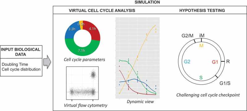 This figure describes the input biological data (doubling time and cell cycle distribution) and the two main outputs of the simulator. The simulator offers several tools to analyze cell cycle progression/distribution and provides a virtual dynamic view of the cell cycle parameters. Moreover, the simulator allows testing hypotheses, such as challenging the cell cycle checkpoints.
Introduction
The discovery of the eukaryotic cell cycle regulatory mechanisms in the late 80s [1–3] has led many researchers to explore the links of various biological processes with the cell cycle in a large panel of biological model systems. Thirty years later, we have now quite a detailed view of the players and regulatory mechanisms that govern cell cycle progression, their connection with embryo development and morphogenesis, their defects in various diseases including cancer, and their therapeutic potential [4].
Modeling and in silico simulation offer additional opportunities to explore biological processes, such as cell cycle and cell proliferation. Models based on the ordinary differential equation (ODE) have been mainly used to study the proliferation [5,6] and the repartition of a cell population in the different phases of the cell cycle [7,8]. The complexity of these models has then been increased by taking into account the molecular network of cyclins [9–11], and the ratio of proliferating versus quiescent cells [12]. However, these approaches are limited when considering the interaction of cells with their local environment (e.g. impact on cell metabolism, proliferation rate…).
Besides ODE, agent-based models also are used to represent cell populations and how the behavior of every single cell influences the whole cell population at a higher scale (i.e. the macroscopic dynamics emerges from the single cell behavior). This approach has the advantage to dissociate the agent behavior (cells) from its physical representation in the virtual environment. With the increase in computing power, it has been possible to bring together models of cell cycle regulation and models of virtual environments [13]. This allows both the simulation of cell physics [14] and the emergence of different gradients (such as oxygen, growth factors, pH, etc.) [15].
Two approaches can be used to model the virtual environment: on-lattice and off-lattice. Off-lattice models are most often employed to study the cell biomechanical properties and their effect on cell growth [14], migration [16–18] and contact inhibition induced by mechanical stress [19,20]. Additional details about off-lattice modeling can be found in [21]. These models present two main limitations: the relatively complex implementation and calibration and the high computational cost.
The second approach (i.e. on-lattice or cellular automata [22]) is commonly used due to its simplicity of implementation [23–27]. Drasdo et al. proposed a broad review of the existing on-lattice models and classified them according to their spatial resolution and the inclusion (or not) of data on the speed of cell movement [28]. In the simplest models, cells are associated uniquely to one lattice site (type B) [29,30]. Conversely, in type A models, cells are grouped within larger size meshes to reduce the computational costs [31]. Type D models are an extension oftype A and take into account also cell motion based on lattice gas cellular automata [32,33]. Finally, in type C models, cells are represented with multiple lattice sites (e.g. cellular Potts models) [34,35].
Here, we present a new computational agent-based model of the cell environment and the cell cycle dynamics. This model is based on a stochastic model of cell progression through the cell cycle. We also propose an alternative representation of the environment that allows considering the local cell density with finer details and its influence on the cell cycle dynamics. According to Drasdo et al. [28], our model can be classified in the type A group because it contains multiple cells per lattice site, but its aim is to offer a finer representation of the cell local density instead of computation efficiency. In this study, we focused on assessing how accurately this cell cycle simulator can reproduce i) the fate of a growing population of HCT116 colon adenocarcinoma cells from log phase to confluence, and ii) the synchronization of cells at the intra-mitotic checkpoint using nocodazole.
Results
An agent-based model to reproduce the cell cycle dynamics of in vitro proliferating colon cancer cells
A cell cycle simulation model must take into account and offer the possibility to manipulate four checkpoints (Figure 1(a), upper panel): the “R” restriction point in the G1 phase that controls commitment to enter the cell cycle based on intra- and extra-cellular mitogenic signals, the G1/S and G2/M checkpoints that are activated upon DNA damage, and the intra-mitotic (iM) checkpoint that prevents abnormal segregation of sister chromatids at mitosis.
Figure 1.
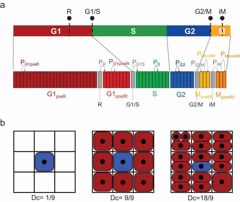
Schematic representation of the cell cycle model (a) Cell cycle model: the cell cycle is modeled by the succession of 10 Bernoulli processes; grey processes correspond to the checkpoints (R, G1/S, G2/M and intraMitotic, iM) and contain only one step. The duration of the other processes is discretized in fixed-time steps, and the number of the resulting steps corresponds to the number of Bernoulli trials that the cell will have to successfully perform to move to the next process. The probability is the probability of success of the Bernoulli draws associated with each process . This allows the regulation of the progression speed in each of the sub-phases. (b) Model of the environment: each of the three panels shows the local environment of the central blue cell at different occupancy stages in its Moore neighborhood, with the corresponding local density indicated.
To model these biological data in the most possible realistic manner, we used agent-based modeling where the agent behaviors are described by using a cell cycle discretized with time steps of Δt duration (6 min in this work). Each cell cycle phase was modeled using one Bernoulli process [36] or two for phases that contain a checkpoint ( and sub-phases) (Figure 1(a), lower panel). To have a single mathematical object to manipulate, each checkpoint also was represented by one Bernoulli process. A Bernoulli process allows implementing a stochastic temporal discretization that in our model represented the temporal progression of cells through each phase or sub-phase of the cell cycle. At each time step, a draw with a given probability (x representing a phase, a sub-phase, or a checkpoint) regulates the progression speed of each process. A Bernoulli process also defines a minimum amount of success, that is necessary to validate the process, and that represents the minimum duration of the phase or sub-phase. A Bernoulli process also integrates the maximum number of attempts before being considered as failed. This parameter was not used in this study (and therefore was set to an infinite value) but could be useful to represent possible cell cycle exits.
Such representation of the cell cycle is generic enough to allow the integration of additional external events. In normal conditions, draw probabilities of all Bernoulli processes are equal to one. To take into account the addition of a drug to the culture medium, nutrient depletion, or any other kind of environmental modifications, the model modifies the draw probability of the Bernoulli process(es) that correspond(s) to the phase(s), sub-phase(s), or checkpoint(s) affected by such event.
Intercellular variability is another key feature that the model must take into account to allow the emergence of asynchronous cell populations [37]. In our model, intercellular variability was modeled by randomly choosing the minimum success amount of each Bernoulli process following a log-normal law [38,39] for each new cell created in the simulation (see Methods for more details).
Virtual cells are inoculated in a two-dimensional (2D) discrete environment represented by a square 3-by-3 lattice (Figure 1(b)). Each position of the grid can contain one or more cells. When cell density is low, each grid position contains at most one cell. A cell succeeding its Bernoulli process will produce a new cell that is added in a free grid position in its Moore neighborhood. As soon as local confluence is reached (i.e. when no free neighboring grid position is available for a dividing cell), the newborn cell is added to the grid position that contains the lowest number of cells in the dividing cell-centered lattice. The local grid position density at any time of the simulation is given by , where is the number of cells in the Moore neighborhood that includes the position of the cell considered at that moment. can be higher than 1.0 to represent the potential capacity of transformed cells to overcome contact inhibition and to reach high densities [40]. The initial cell population is uniformly distributed in the grid without cell stacking.
Calibration of the cell cycle simulation model
The cell type-specific input data required to run the cell cycle simulator are: (i) the doubling time, and (ii) the cell cycle phase distribution of the exponentially growing cell population under study. In the example presented here, these data were obtained by monitoring the proliferation of colon adenocarcinoma HCT116 cells. To ensure an accurate determination of the percentage of cells in each cell cycle phase, particularly in S-phase, the cell cycle distribution was determined by flow cytometry after HCT116 cell labeling with 5-ethylnyl-2'-deoxyuridine (EdU), a thymidine nucleoside analogue that is incorporated in the DNA of cells in S phase, and with the 3–12-I-22 antibody that recognizes specifically mitotic cells [41] (see Methods), at various time points between seeding and confluence. These flow cytometry data (total number of cells and percentage of cells in the different phases at each time point; supplementary Figure S1) were used to calculate the mean percentage of cells in each cell cycle phase during exponential growth (Figure 2(a)). Data on the doubling time and the cell cycle phase distribution can then be used to determine the actual duration of each phase. However, this determination is often based on a conventional error that consists in directly allocating the phase duration in function of the percentage of cells in each phase and proportionally to the doubling time. This is an erroneous calculation: the duration of the cell cycle phases must be determined by considering that the cell age distribution in the cell cycle follows an exponentially decreasing distribution because of the division into two daughter cells at each mitosis [42]:
| (1) |
Figure 2.
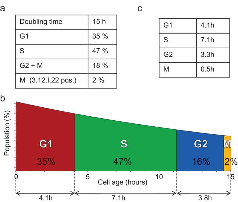
Settings of the cell cycle model (a) Cell cycle distribution of exponentially growing HCT116 cells (experimental data). These input data were extracted from the data collected in the log phase of the experiment shown in Supplementary Figure S1. (b) Cell cycle and age distribution of an exponentially growing HCT116 cell population. The colored areas under the curve indicate the distribution of the cells in each phase (in percentage) according to [42]. On the lower line are indicated the deduced phase durations (in hours). (c) Table showing the duration of each cell cycle phase in exponentially growing HCT116 cells deduced from the representation presented in panel (b).
where is the percentage of cells of age and is the doubling time.
This distribution allows determining the phase duration when knowing the doubling time and cell phase repartition. However, this equation does not consider the M-phase on its own, but only a G2-M phase. Therefore, we adapted this model to calculate the duration of all cell cycle phases:
| (2) |
where , , and are the duration of the respective phases, and ,, and are the rate of cells in the respective phases obtained by flow cytometry during exponential growth (Figures 2(b and c)).
Note that the M phase duration was based on the duration of the cell positivity for the 3–12-I-22 antibody that is restricted to the prophase-metaphase/anaphase transition [41], and not to the actual whole duration of mitosis from early prophase to the end of cytokinesis.
Simulating the changes in cell cycle distribution of a cell population that progressively reaches confluence
It is largely acknowledged that cell confluence directly influences cell progression through the “R” restriction point, which in turn leads to an increase in the duration of the G1 phase. Therefore, we tested whether the in silico model could reproduce the proliferation kinetics and the associated cell cycle parameter changes of a population of HCT116 cells from the initial log phase to confluence.
To represent this in our model, we developed a workflow that directly correlates data on confluence (i.e. percentage of the dish surface covered by cells) to the G1 phase duration. This workflow is graphically represented in Supplementary Figure S2.
The first step of the workflow consisted in determining the cell density per unit of surface in optimal culture conditions (i.e. when not subject to any mechanical stress). The unit of surface corresponds to the surface occupied by a cell with no mechanical constraint, and is calculated as follows:
| (3) |
where represents the confluence, and the number of cells in the culture dish in optimal conditions. In this study, the optimal condition was at 24 h after inoculation when cell confluence was 16.4%.
Based on this initial value, we then calculated the global optimal density at any culture time point with:
| (4) |
where is the number of cells. This density measure takes into account the capacity of transformed cancer cells to overlap.
By considering the hypothesis that the effect of high cell density induces a slowdown at the “R” checkpoint, we could directly correlate density data at any time of the culture, calculated as shown above, with the flow cytometry data that provided the percentage of cells in G1:
| (5) |
We then analyzed by flow cytometry HCT116 cells at different time points up to 4 days after seeding, and determined the percentage of cells in the G1, S and G2-M phases, as before (Figure 3). These data highlighted the cell cycle distribution changes associated with increasing cell confluence. On the basis of the data on the cell cycle distribution of this asynchronous population of HCT116 cells (section 2.2) and by assuming that the duration of the S, G2 and M phases was not substantially modified by density, we could use the percentage of cells in the G1 phase to calculate the G1 elongation with the following formula (see Figure 4 for a graphical presentation):
| (6) |
Figure 3.
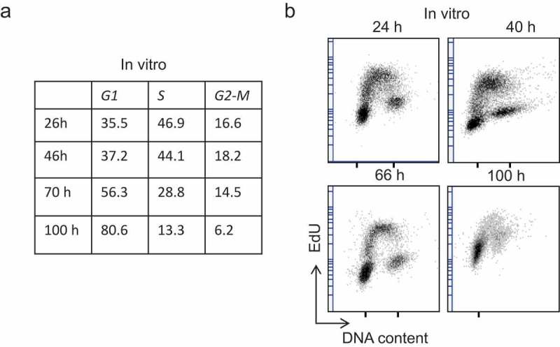
Experimental data from an exponentially growing HCT116 cell population Variation of the cell cycle distribution in HCT116 cells over time. At the indicated time points during culture, the cell cycle distribution was analyzed by flow cytometry after DNA staining with the DRAQ-5 fluorescent probe and labeling of S-phase cells with EdU (30 min pulse). (a) Percentage of cells in each cell cycle phase, and (b) dot plots showing the DNA content and EdU labeling at different time points.
Figure 4.
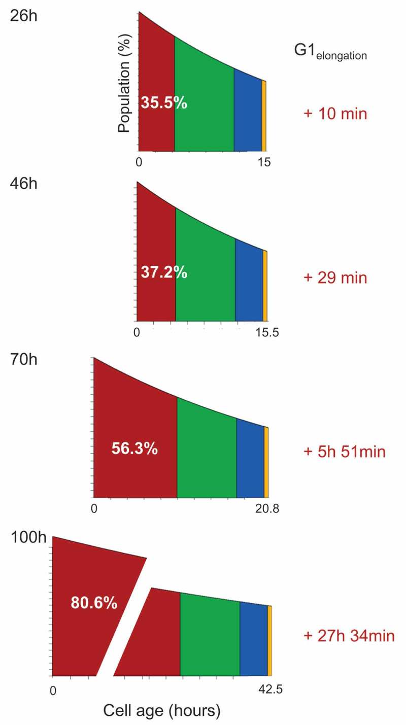
In silico determination of G1 elongation Graphical representation of the G1 phase elongation induced by the increasing cell confluence. The percentage of cells in the G1 phase of the cell cycle can be converted into the duration of G1 phase elongation. It was assumed that the duration of the S, G2 and M phases did not change.
where is the duration of the phase, and is the population doubling time in an exponentially growing culture. At 100 h after seeding, the increase in the G1 phase rate corresponded to a G1 elongation of 27 h and 34 min compared with the time 0 (Figure 4).
To integrate this piece of information into the cell cycle simulation model, we needed to determine the probability of the Bernoulli process to achieve the desired elongation. This probability is given by the following formula:
| (7) |
where is the duration of the sub-phase in an exponentially growing culture.
The in silico simulation using this specific workflow to obtain a cell cycle phase distribution approximately at the same time points as those used experimentally gave similar cell cycle repartitions as observed in vitro (Figure 5(a) and compare with Figure 3(a)), and accurately determined the distribution changes over time. We also compared the experimental results and the in silico bi-parametric representation (EdU labeling – DNA content). The experimental data showed the decrease in cells in the S and G2-M phases, and the accumulation of cells in G1 over time (i.e. progressive increase in cell confluence (Figure 3(b)). As the simulation was based on the position of actual individual cells within the cell cycle, the simulator provided data that could be used to generate a virtual representation of the EdU incorporation analysis relative to the DNA content (Figure 5(b)). We added a random noise to the data (see Methods) to make the representation looking like the output biologists are familiar with.
Figure 5.
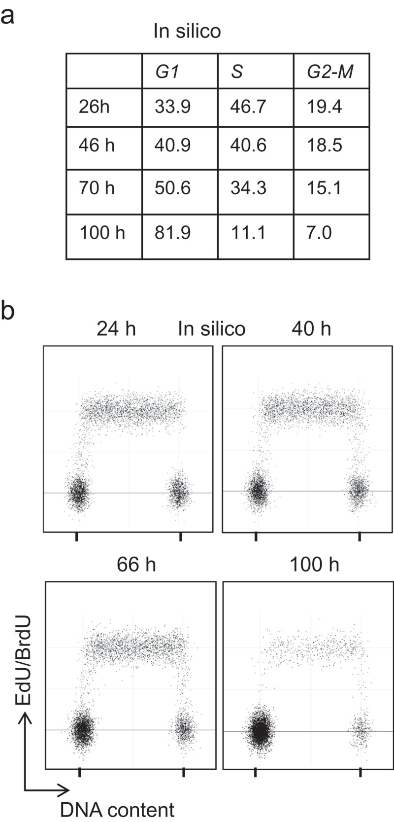
Simulation data of a growing HCT116 cell population In silico simulation of the variation of HCT116 cell cycle distribution. (a) Average percentage of cells in each phase from 50 simulations, and (b) Simulated dot plots of DNA content (with additive white Gaussian noise, SD = 0.05) and EdU-positive cells (with additive white Gaussian noise, SD = 0.1).
Simulation of mitotic arrest using nocodazole
We next examined whether the cell cycle simulator could reproduce the effects of incubation with nocodazole, a drug that impairs microtubule dynamics, resulting in mitotic cell cycle arrest through the activation of the intra-mitotic spindle assembly checkpoint [43,44].
First, we compared the proliferation of exponentially growing HCT116 cells after incubation with 200 ng/ml nocodazole (in vitro experiments) and the model output after tightly preventing the progression of any individual cell through the intra-mitotic checkpoint (iM). For the in vitro experiments, we checked that this nocodazole concentration resulted in checkpoint activation that could be reversed upon drug removal and that the effect was strong enough to impair mitotic slippage and/or apoptosis entry up to 30 h after treatment (data not shown).
Flow cytometry analysis after DNA staining and labeling of mitotic cells (Figure 6(a), colored dots; and Figure 7(a)) showed that nocodazole-treated cells progressively exited the G1, S and G2 phase and accumulated in mitosis (more than 85% of cells after 20 h). In agreement, EdU pulse labeling indicated that the number of cells in S phase progressively decreased (see supplementary Figure S3A).
Figure 6.
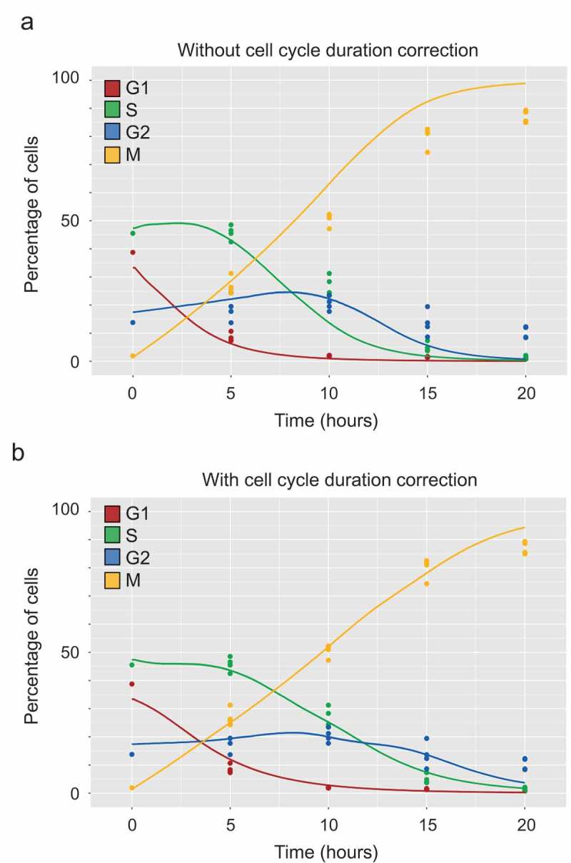
Comparison of in vitro and in silico results after nocodazole synchronization (a, b) Colored dots (experimental data): Exponentially growing HCT116 cells were incubated with 200 ng/ml nocodazole for 20 h. The cell cycle repartition was analyzed by flow cytometry after DNA labeling with DRAQ-5 and detection of mitotic cells using a specific monoclonal antibody [41]. The obtained triplicate results are represented by dots of different colors for each phase. Colored curves (in silico data): average phase distribution obtained from 50 simulations. (a) Comparison of the experimental (dots) and in silico results (curves) obtained by modeling nocodazole effect as a complete block of the iM checkpoint (. (b) Comparison of the experimental (dots) and in silico results (curves) obtained by modeling nocodazole as a non-permissive block of the iM checkpoint () with the elongation of the other phases (, and ) that was determined by sampling the Bernoulli probabilities . The figure reports the parameters that best fit the experimental data (see Materials and Methods for additional explanations).
Figure 7.
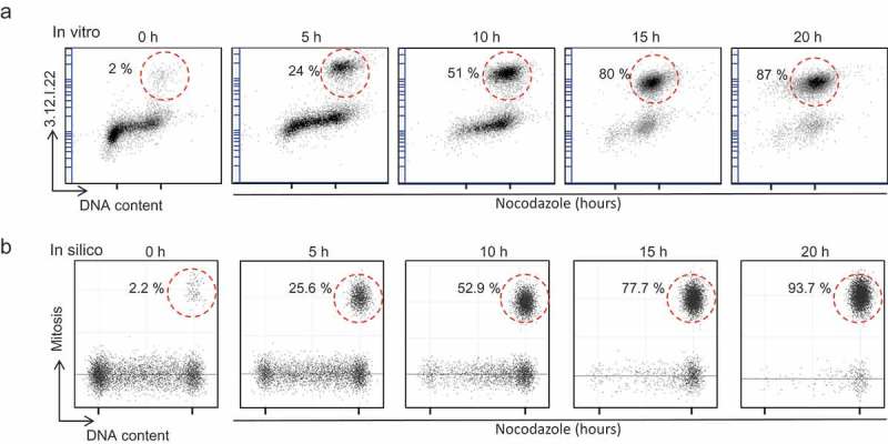
The cell cycle simulator reproduces the cell cycle arrest in mitosis of HCT116 cells incubated with nocodazole (a) In vitro data: Exponentially growing HCT116 cells were incubated with nocodazole for 20 h, like in Figure 4. Dot plot representation of the cell cycle distribution obtained by flow cytometry analysis after DNA staining with DRAQ-5 and labeling of mitotic cells with the 3.12.I.22 antibody. (b) In silico simulation: simulated dot plots of the DNA content and mitotic cell labeling.
Comparison of the results obtained with the in silico simulator (curves) with the in vitro data (dots) (Figure 6(a)) showed that the simulation led to a faster accumulation of cells in mitosis and a faster reduction of the percentage of S- and G2-phase cells. Therefore, we investigated various hypotheses to explain this discrepancy between in silico and in vitro data. To this aim, we explored a large number of combinations of Bernoulli process probabilities that were directly associated with phase duration in the model, to find the one fitting with the experimental data (for more details, see the Methods section). We obtained the following elongation values for the fittest set of parameters:, and . Finally, the model could accurately reproduce the activation of the intra-mitotic checkpoint only when the different phases of the cell cycle were elongated of a given amount of time. The underlying rationale was that nocodazole not only arrested cells in mitosis but also resulted in a delayed progression of the other phases of the cell cycle. Altogether, the results presented in Figure 6(b), Figure 7 and supplementary Figure S3 indicated that, with these modified parameters, the simulator accurately reproduced the activation of the intra-mitotic checkpoint with cell cycle arrest in M-phase and the progressive consequences on cell cycle distribution. This was in agreement with the hypothesis that in HCT116 cells, nocodazole affected not only the M phase but also slowed down the entire cell cycle. Moreover, while in vitro experiments only allowed the analysis of discrete time-points during the course of the experiment, in silico simulations offered the possibility to monitor the cell cycle distribution variations and the progressive accumulation of cells in mitosis during the whole duration of the experiment. Such a dynamic view of the progressive modifications of the cell cycle represents a major asset of the simulation compared with the in vitro experiment.
Discussion
In the work reported here, we present an in silico model that reproduces the dynamics of a proliferating HCT116 colon cancer cell population. We demonstrated that this model can simulate the progressive confluence and the associated G1-phase elongation. We also modeled in silico the synchronization of cells in mitosis using nocodazole to demonstrate that this cell cycle simulator can reproduce the nocodazole-induced cell cycle arrest at the metaphase-anaphase checkpoint. Finally, the simulator highlighted that in HCT116 cells, nocodazole slows down the entire cell cycle in addition to arresting cells in the M phase. We believe this model can be useful for cell biologists to explore hypotheses and address fundamental questions on the mechanisms that regulate cell behavior in culture wells but that are hard to explore with the available experimental protocols [45].
The cell cycle simulator presented in this paper is generic and can be adapted to many different cell lines. Its wide usability is also strengthened by the fact that the experimental data required to calibrate the model can be acquired with straightforward experiments, mostly based on flow cytometry analyses.
In addition, our cell cycle simulator is modular because the different parts of the model (cell environment, confluence variations/effects, effect of a drug, etc.) can be plugged or unplugged, depending on the question under investigation. Therefore, the model calibration can be facilitated/simplified by focusing only on the features that are crucial for the question under study.
Agent-based modeling allows the easy incorporation of new drugs or new environmental conditions (oxygen, nutriments, growth factors, etc.) that may influence a specific cell cycle phase or checkpoint. As shown here, this modeling method is fairly flexible and, while designing the model of the new feature to consider can be challenging, its integration into the whole model is usually straightforward.
As only a few experimental data are required to feed and parameterize the cell cycle simulator, it will be possible to easily calibrate and use it for various cell types. One could simulate the proliferation of normal untransformed cells and their specific features. For instance, for primary fibroblasts, the maximum occupancy parameter on the grid (Figure 1(b)) should be set to 9/9 to take into account the stringency of the confluence effect on their proliferation. Conversely, specific gene mutations in a cancer cell line may facilitate the bypass of a checkpoint. Our simulator can handle such specificities by tuning up or down the stringency of a given checkpoint simply by changing the probability of the associated Bernoulli process. For instance, the inhibition of the pRB pathway could be easily simulated by switching off totally or partially the “R” commitment checkpoint. A similar approach could also be used to simulate exposure to a drug at a concentration that is not sufficient to fully arrest the cell cycle (for instance, a very low concentration of a microtubule-targeting poison, such as nocodazole or paclitaxel).
A major interest of this simulation model resides in the possibility to explore cell cycle features through the comparison of experimental data and simulated outputs. As exemplified in this report, the deleterious effect of nocodazole on cell cycle progression is never considered when this drug is used for cell synchronization. Here, we found that initially, the simulation results did not match the experimental data because this nocodazole “side” effect was not taken into account. Indeed, by slowing down cell progression in interphase, nocodazole led to a longer duration of the cell cycle. The introduction of this parameter in the model was sufficient to match the in vitro data and the simulation data. Thus, the use of our simulator opens the possibility to predict and explore unexpected features.
A major challenge for cell cycle researchers is to detect and monitor events that occur at very discrete and specific stages of the cell cycle in a large population of asynchronous cells. The natural synchronization of the first embryonic cell cycles [46,47] and the simplicity of the use of thermosensitive mutants in yeasts [48–50] contributed to their wide and fruitful use. This is not the case for animal cells in culture that are fully asynchronous and require synchronization methods based on laborious experimental protocols. Assistance from the researchers on the details of their experimental protocol, such as the timing of addition and withdraw of the synchronizing drug, will be of tremendous help for fine-tuning our cell cycle simulator for each user’s specific needs. Thus, we anticipate that with future developments, the simulator presented in this report could become the basis for a simulation tool that will be made available through a web interface to the cell cycle research community.
Finally, in real life, cells do not proliferate as 2D monolayers in Petri dishes but are organized in 3D tissues that are assembled in organs. The next step in the development of our proliferation/cell cycle simulator will be to implement all the complexity of 3D cell proliferation with the integration of interactions between cells and the matrix, as well as nutrient and oxygen gradients to reproduce the regionalization of cell proliferation that is a key feature of tissue homeostasis.
Materials and methods
Cell culture
HCT116 colon adenocarcinoma cells (ATCC) were cultured in Dulbecco’s modified Eagle Medium (Gibco, Life Technologies) supplemented with 10% fetal calf serum (Gibco, Life Technologies) and 1% penicillin/streptomycin (100 U/mL, Gibco, Life Technologies) in a humidified atmosphere of 5% CO2 at 37°C. Nocodazole was purchased from Sigma Aldrich and used at the final concentration of 200 ng/ml.
Flow cytometry
Flow cytometry analysis of cell cycle distribution was performed according to the general recommendations [51] using an ACCURI C6 (BD) flow cytometer. HCT116 cells were harvested and fixed in 10% neutral buffered formalin solution (Sigma Aldrich). DNA was stained with DRAQ5 (Invitrogen). To detect cells in S-phase, EdU (10 µM) was added to the culture medium 30 min before harvesting. EdU incorporation analysis was performed following the manufacturer’s instructions by using the Click-it® EdU Alexa Fluor® Imaging Kit (Molecular Probes) that is based on a “click” reaction between EdU and the Alexa Fluor® 488 dye. Mitotic cells were detected after staining with the monoclonal antibody 3.12.I.22 [41] that was revealed using Alexa Fluor 488-conjugated antibodies.
In silico intercellular variability
The intercellular variability was modeled by randomly choosing the minimum success amount of each Bernoulli process following a log-normal law for each new cell created in the simulation. The mean value of the law was based on experimental data on the population doubling time (total duration of the cell cycle) and cell cycle phases (by flow cytometry) in exponential growth conditions. As the G1 phase is responsible for most of the cell cycle variability [52], the standard deviations of the sub-phases and were set to 90% of the average, and the other phases and sub-phases were set to 10% of the average. These values were obtained by parameter sampling on the standard deviation used for the different log-normal distribution laws (for each Bernoulli process) to fit as best as possible with the single cell cycle duration measurements obtained by time-lapse video-microscopy (data not shown).
Determination of the cell cycle parameters in cells incubated with nocodazole
Parameter sampling was performed to determine which parameter set fits best the experimental data. The exploration domain was defined in terms of hours of elongation that were converted for the model into the probability of success of Bernoulli processes by using the following equation:
where is the probability of the processes in phase , the average duration of phase and the desired elongation for phase .
The exploration domain was defined between 0 and 4 h with a step of 6 min for each phase, for a total of 68,921 simulations. Then, the least squares method was used with the results of these simulations to determine the parameter set that minimizes the following sum:
where is the experimental measurement of the percentage of cells in phase p at time t, and is the simulated measurement of the percentage of cells in phase p at time t with the parameters (i.e. the elongation of the G1, S and G2 phases, respectively, induced by nocodazole).
Acknowledgments
We are grateful to the members of our group for their interest in this project. The authors thank Elisabetta Andermarcher for expert manuscript editing. The support of the staff of the ITAV imaging facility is gratefully acknowledged. The authors wish to acknowledge TRI-Genotoul facilities. DB was a doctoral student fellow supported by the Région Midi-Pyrénées and Université Toulouse Capitole. This work was financially supported by the CNRS and the University of Toulouse III.
Disclosure statement
No potential conflict of interest was reported by the authors.
Supplementary material
Supplemental data for this article can be accessed here.
References
- [1].Hartwell LH. Cell division from a genetic perspective. J Cell Biol. 1978;77:627–637. [DOI] [PMC free article] [PubMed] [Google Scholar]
- [2].Hunt T. Maturation promoting factor, cyclin and the control of M-phase. Curr Opin Cell Biol. 1989;1:74–286. [DOI] [PubMed] [Google Scholar]
- [3].Nurse P. Universal control mechanism regulating onset of M-phase. Nature. 1990;344:503–508. [DOI] [PubMed] [Google Scholar]
- [4].Sherr CJ, Beach D, Shapiro GI. Targeting CDK4 and CDK6: from discovery to therapy. Cancer Discov. 2016;6:353–367. [DOI] [PMC free article] [PubMed] [Google Scholar]
- [5].Bell GI, Anderson EC. Cell growth and division. I. A mathematical model with applications to cell volume distributions in mammalian suspension cultures. Biophys J. 1967;7:329–351. [DOI] [PMC free article] [PubMed] [Google Scholar]
- [6].Basse B, Ubezio P. A generalised age- and phase-structured model of human tumour cell populations both unperturbed and exposed to a range of cancer therapies. Bull Math Biol. 2007;69:1673–1690. [DOI] [PubMed] [Google Scholar]
- [7].Sasane S. An age structured cell cycle model with crowding. J Math Anal Appl. 2016;444:768–803. [Google Scholar]
- [8].Basse B, Baguley BC, Marshall ES, et al. A mathematical model for analysis of the cell cycle in cell lines derived from human tumors. J Math Biol. 2003;47:295–312. [DOI] [PubMed] [Google Scholar]
- [9].Novak B, Tyson JJ. Numerical analysis of a comprehensive model of M-phase control in Xenopus oocyte extracts and intact embryos. J Cell Sci. 1993;106(Pt 4):1153–1168. [DOI] [PubMed] [Google Scholar]
- [10].Tomasoni D, Lupi M, Brikci FB, et al. Timing the changes of cyclin E cell content in G1 in exponentially growing cells. Exp Cell Res. 2003;288:158–167. [DOI] [PubMed] [Google Scholar]
- [11].Gerard C, Tyson JJ, Coudreuse D, et al. Cell cycle control by a minimal Cdk network. PLoS Comput Biol. 2015;11:e1004056. [DOI] [PMC free article] [PubMed] [Google Scholar]
- [12].Spinelli L, Torricelli A, Ubezio P, et al. Modelling the balance between quiescence and cell death in normal and tumour cell populations. Math Biosci. 2006;202:349–370. [DOI] [PubMed] [Google Scholar]
- [13].Zhang L, Athale CA, Deisboeck TS. Development of a three-dimensional multiscale agent-based tumor model: simulating gene-protein interaction profiles, cell phenotypes and multicellular patterns in brain cancer. J Theor Biol. 2007;244:96–107. [DOI] [PubMed] [Google Scholar]
- [14].Drasdo D, Hohme S. A single-cell-based model of tumor growth in vitro: monolayers and spheroids. Phys Biol. 2005;2:133–147. [DOI] [PubMed] [Google Scholar]
- [15].Jiang Y, Pjesivac-Grbovic J, Cantrell C, et al. A multiscale model for avascular tumor growth. Biophys J. 2005;89:3884–3894. [DOI] [PMC free article] [PubMed] [Google Scholar]
- [16].Zhu J, Mogilner A. Comparison of cell migration mechanical strategies in three-dimensional matrices: a computational study. Interface Focus. 2016;6:20160040. [DOI] [PMC free article] [PubMed] [Google Scholar]
- [17].Tozluoglu M, Tournier AL, Jenkins RP, et al. Matrix geometry determines optimal cancer cell migration strategy and modulates response to interventions. Nat Cell Biol. 2013;15:751–762. [DOI] [PubMed] [Google Scholar]
- [18].Kim MC, Neal DM, Kamm RD, et al. Dynamic modeling of cell migration and spreading behaviors on fibronectin coated planar substrates and micropatterned geometries. PLoS Comput Biol. 2013;9:e1002926. [DOI] [PMC free article] [PubMed] [Google Scholar]
- [19].Byrne H, Drasdo D. Individual-based and continuum models of growing cell populations: a comparison. J Math Biol. 2009;58:657–687. [DOI] [PubMed] [Google Scholar]
- [20].Schaller G, Meyer-Hermann M. Multicellular tumor spheroid in an off-lattice Voronoi-Delaunay cell model. Phys Rev E Stat Nonlin Soft Matter Phys. 2005;71:051910. [DOI] [PubMed] [Google Scholar]
- [21].Van Liedekerke P, Buttenschon A, Drasdo D. Off-lattice agent-based models for cell and tumor growth: numerical methods, implementation, and applications In: Cerrolaza M, Shefelbine S, Garzón-Alvarado D, editors. Numerical methods and advanced simulation in biomechanics and biological processes. Elsevier; 2018. p. 245–267. [Google Scholar]
- [22].Von Neumann J. Theory of self-reproducing automata. Champaign (IL): University of Illinois Press; 1966. [Google Scholar]
- [23].Kansal AR, Torquato S, Harsh IG, et al. Cellular automaton of idealized brain tumor growth dynamics. Biosystems. 2000;55:119–127. [DOI] [PubMed] [Google Scholar]
- [24].Engelberg JA, Ropella GE, Hunt CA. Essential operating principles for tumor spheroid growth. BMC Syst Biol. 2008;2:110. [DOI] [PMC free article] [PubMed] [Google Scholar]
- [25].Patel AA, Gawlinski ET, Lemieux SK, et al. A cellular automaton model of early tumor growth and invasion. J Theor Biol. 2001;213:315–331. [DOI] [PubMed] [Google Scholar]
- [26].Gatenby RA, Smallbone K, Maini PK, et al. Cellular adaptations to hypoxia and acidosis during somatic evolution of breast cancer. Br J Cancer. 2007;97:646–653. [DOI] [PMC free article] [PubMed] [Google Scholar]
- [27].Piotrowska MJ, Angus SD. A quantitative cellular automaton model of in vitro multicellular spheroid tumour growth. J Theor Biol. 2009;258:165–178. [DOI] [PubMed] [Google Scholar]
- [28].Drasdo D, Buttenschon A, Van Liedekerke P. Agent-based lattice models of multicellular systems: numerical methods, implementation, and applications In: Cerrolaza M, Shefelbine S, Garzón-Alvarado D, editors. Numerical methods and advanced simulation in biomechanics and biological processes. Elsevier; 2018. p. 223–238. [Google Scholar]
- [29].Jagiella N, Muller B, Muller M, et al. Inferring growth control mechanisms in growing multi-cellular spheroids of NSCLC cells from spatial-temporal image data. PLoS Comput Biol. 2016;12:e1004412. [DOI] [PMC free article] [PubMed] [Google Scholar]
- [30].Yates CA, Baker RE. Isotropic model for cluster growth on a regular lattice. Phys Rev E Stat Nonlin Soft Matter Phys. 2013;88:023304. [DOI] [PubMed] [Google Scholar]
- [31].Drasdo D. Coarse graining in simulated cell populations. Adv Complex Syst. 2005;8:319–363. [Google Scholar]
- [32].Bottger K, Hatzikirou H, Chauviere A. Investigation of the migration/proliferation dichotomy and its impact on avascular glioma invasion. Math Modell Nat Phenom. 2012;7:105–135. [Google Scholar]
- [33].Tektonidis M, Hatzikirou H, Chauviere A, et al. Identification of intrinsic in vitro cellular mechanisms for glioma invasion. J Theor Biol. 2011;287:131–147. [DOI] [PubMed] [Google Scholar]
- [34].Tripodi S, Ballet P, Rodin V. Computational energetic model of morphogenesis based on multi-agent cellular potts model. Adv Exp Med Biol. 2010;680:685–692. [DOI] [PubMed] [Google Scholar]
- [35].Boghaert E, Radisky DC, Nelson CM. Lattice-based model of ductal carcinoma in situ suggests rules for breast cancer progression to an invasive state. PLoS Comput Biol. 2014;10:e1003997. [DOI] [PMC free article] [PubMed] [Google Scholar]
- [36].Pascalie J, Lobjois V, Luga H, Ducommun Y, Duthen Y. A Checkpoint-Orientated Model to Simulate Unconstrained Proliferation of Cells (regular paper). European Conference on Artificial Life (ECAL 2011), 09/08/2011-12/08/2011. Paris: The MIT Press; 2018. p. 630-637. [Google Scholar]
- [37].Chiorino G, Metz JA, Tomasoni D, et al. Desynchronization rate in cell populations: mathematical modeling and experimental data. J Theor Biol. 2001;208:185–199. [DOI] [PubMed] [Google Scholar]
- [38].Ubezio P. Cell cycle simulation for flow cytometry. Comput Methods Programs Biomed. 1990;31:255–266. [DOI] [PubMed] [Google Scholar]
- [39].Sherer E, Tocce E, Hannemann RE, et al. Identification of age-structured models: cell cycle phase transitions. Biotechnol Bioeng. 2008;99:960–974. [DOI] [PubMed] [Google Scholar]
- [40].Hanahan D, Weinberg RA. Hallmarks of cancer: the next generation. Cell. 2011;144:646–674. [DOI] [PubMed] [Google Scholar]
- [41].Cazales M, Quaranta M, Lobjois V, et al. A new mitotic-cell specific monoclonal antibody. Cell Cycle. 2008;7:267–268. [DOI] [PubMed] [Google Scholar]
- [42].Priori L, Ubezio P. Mathematical modelling and computer simulation of cell synchrony. Methods Cell Sci. 1996;18:83–91. [Google Scholar]
- [43].Ma HT, Poon RY. Synchronization of HeLa cells. Methods Mol Biol. 2011;761:151–161. [DOI] [PubMed] [Google Scholar]
- [44].Uzbekov R, Chartrain I, Philippe M, et al. Cell cycle analysis and synchronization of the Xenopus cell line XL2. Exp Cell Res. 1998;242:60–68. [DOI] [PubMed] [Google Scholar]
- [45].Tyson JJ, Novak B. Models in biology: lessons from modeling regulation of the eukaryotic cell cycle. BMC Biol. 2015;13:46. [DOI] [PMC free article] [PubMed] [Google Scholar]
- [46].O’Farrell PH, Edgar BA, Lakich D, et al. Directing cell division during development. Science. 1989;246:635–646. [DOI] [PubMed] [Google Scholar]
- [47].Kirschner MW, Newport J, Gerhart JC. The timing of early developmental events in Xenopus. Trends Genet. 1985;1:41–47. [Google Scholar]
- [48].Beach D, Durkacz B, Nurse P. Functionally homologous cell cycle control genes in budding and fission yeast. Nature. 1982;300:706–709. [DOI] [PubMed] [Google Scholar]
- [49].Creanor J. Preparation of synchronous cultures of the fission yeast In: Pagano M, editor. Cell cycle - materials and methods. New York: Springer-Verlag; 1995. p. 132–144. [Google Scholar]
- [50].Hartwell LH. Saccharomyces cerevisiae cell cycle. Bacteriol Rev. 1974;38:164–198. [DOI] [PMC free article] [PubMed] [Google Scholar]
- [51].Darzynkiewicz Z. Mammalian cell-cycle analysis In: Fantes P, Brooks R, editors. The cell cycle: a practical approach. New York: Oxford University Press; 1993. p. 45–67. [Google Scholar]
- [52].Sisken JE, Morasca L. Intrapopulation kinetics of the mitotic cycle. J Cell Biol. 1965;25:179–189. [DOI] [PMC free article] [PubMed] [Google Scholar]
Associated Data
This section collects any data citations, data availability statements, or supplementary materials included in this article.