Model-based and Model-free Techniques for Amyotrophic Lateral Sclerosis Diagnostic Prediction and Patient Clustering

Abstract

Background:

Amyotrophic lateral sclerosis (ALS) is a complex progressive neurodegenerative disorder with an estimated prevalence of about 5 per 100,000 people in the United States. In this study, the disease progression of ALS is measured by the change of Amyotrophic Lateral Sclerosis Functional Rating Scale (ALSFRS) score over time. The study aims to provide clinical decision support for timely forecasting of the ALS trajectory as well as accurate and reproducible computable phenotypic clustering of participants.

Methods:

Patient data are extracted from DREAM-Phil Bowen ALS Prediction Prize4Life Challenge data, most of which are from the Pooled Resource Open-Access ALS Clinical Trials Database (PRO-ACT) archive. We employed model-based and model-free machine-learning methods to predict the change of the ALSFRS score over time. Using training and testing data we quantified and compared the performance of different techniques. We also used unsupervised machine learning methods to cluster the patients into separate computable phenotypes and interpret the derived subcohorts.

Results:

Direct prediction of univariate clinical outcomes based on model-based (linear models) or model-free (machine learning based techniques – random forest and Bayesian adaptive regression trees) was only moderately successful. The correlation coefficients between clinically observed changes in ALSFRS scores relative to the model-based/model-free predicted counterparts were 0.427 (random forest) and 0.545(BART). The reliability of these results were assessed using internal statistical cross validation and well as external data validation. Unsupervised clustering generated very reliable and consistent partitions of the patient cohort into four computable phenotypic subgroups. These clusters were explicated by identifying specific salient clinical features included in the PRO-ACT archive that discriminate between the derived subcohorts.

Conclusions:

There are differences between alternative analytical methods in forecasting specific clinical phenotypes. Although predicting univariate clinical outcomes may be challenging, our results suggest that modern data science strategies are useful in clustering patients and generating evidence-based ALS hypotheses about complex interactions of multivariate factors. Predicting univariate clinical outcomes using the PRO-ACT data yields only marginal accuracy (about 70%). However, unsupervised clustering of participants into sub-groups generates stable, reliable and consistent (exceeding 95%) computable phenotypes whose explication requires interpretation of multivariate sets of features.

Graphical Abstract

Introduction

Prior clinical studies pooling heterogeneous datasets across sites and sources have been successful in examining, simulating and modeling disease progression patterns, e.g., studies of Alzheimer’s disease [1–3] and Parkinson’s disease [4, 5]. Recently, similar effort has been made to integrate all available Amyotrophic Lateral Sclerosis (ALS) clinical information. The Pooled Resource Open-Access ALS Clinical Trials (PRO-ACT) (https://nctu.partners.org/ProACT/) [6] database collects and aggregates clinical data of 16 ALS clinical trials and one observational study completed in the recent twenty years [7]. These big data initiatives to better characterize ALS are ongoing and have the potential to provide insight into disease progression and heterogeneity. While PRO-ACT includes clinical variables on a large number of participants, other programs such as Answer ALS are incorporating “omics” and even wearables data. As ALS enters the era of big data, we utilized the PRO-ACT dataset to help explore the differences in analytical techniques, potential pitfalls, and how these methods can be leveraged in the future. These initiatives, especially when pulled from electronic medical record systems, require acquiring raw data, computational preprocessing, aggregation, harmonization, analysis, and visualization leading to clinically relevant result interpretation. We report on building such workflow that is tested to examine complex ALS data. Next, we employ model-based methods and model-free machine learning techniques for automated disease progression tracking in ALS patients and discuss the relative strengths/weakness of each.

Statistical Model-based vs. Data Science Model-free Methods

Model-based and model-free techniques represent complementary approaches for predictive big data analytics [8]. The former class of techniques includes classical parametric models under some of the following specific assumptions: time series analyses assume model parameters are constant over time, residuals are homoscedastic, and stationarity over some order, and use historic or training data to capture trends or patterns and extrapolate prospective or forecast future observations. Other examples of model-based methods include (1) multivariate regression methods [9], which represent variable interdependencies between predictors and responses in terms of some base functions (e.g., polynomials) whose coefficients capture the influence of all variables on the outcomes and facilitate forward predictions, (2) generalized estimating equations models [10] is a semiparametric technique for population-average inference, rather than subject-specific inference in the linear models, and structural equation models [11], which assume asymmetric causal relationships among normally distributed interval-level measured variables. In general, model-based methods are contingent on many (parametric) assumptions that may not be satisfied in many situations, particularly with heterogeneous sources of data.

Alternatively, model-free machine-learning techniques [12], classification theory [13], network analysis [14], and hierarchical clustering [15] may be employed for unsupervised data mining [16], hyperparameter tuning [17, 18], pattern recognition [19], trend identification [20], k-means [21] or fuzzy [22] clustering. Contrary to the reductionist approach of reality-simplification employed in the model-based methods, model-free techniques combine, evolve, ensemble and train algorithms that adapt to the contextual affinities of a process learning the dynamic characteristics that may explain the observations. Just like with cognitive and social brain development, maturation and aging, model-free techniques may need to be constantly adjusted and are not guaranteed to always be correct. However, when properly trained, effectively maintained, and continuously reinforced, model-free learning based methods provide powerful and reliable forecasting for complex phenomena.

Model-based statistical estimation relies on training data to estimate concrete parameters, like model coefficients, that are explicitly assumed to be included in a specific analytical framework representing a proxy of the underlying process (e.g., GEE, SEM, LASSO, etc.) In contract, model-free inference does not rely on a predetermined analytical framework as a fixed stereotypic representation of the problem. Rather, model-free techniques adapt their structure to the characteristics of the specific data they emulate. For instance, in this context, random forests and decision trees are model-free techniques, as the topology of the graphical networks, as well as the actual branching rules, are freely determined by the data affinities, instead of being prescribed in advance by a specific graph model. Similarly, whereas some clustering techniques are model-based, e.g., Gaussian mixture models, others do not have an apriori structure and rely simply on data affinities, manifold distance measures, or entropy information criteria to group cases into clusters.

In principle, no technique, algorithm, or an approach is really completely model-free, as there are always underlying axiomatic assumptions or characterizations that are expected in all scientific settings. However, the degree to which a specific technique relies on a strict rendition of its analytical representation does divide model-based analyses from model-free inferential approaches. Solving constrained or unconstrained linear models is rather different from solving non-convex machine-learning optimization problems [23–25]. The solutions to many model-based problems are largely consistent and reproducible, and can be obtained in polynomial time [26]. Model-free solutions to non-convex problems may be NP-hard, frequently rely on heuristics, and may be unstable [27, 28].

Prior ALS predictive modeling studies

In a previous DREAM-Phil Bowen ALS Prediction Prize4Life crowdsourcing challenge [29], teams of investigators developed several promising predictive models based on the clinical database PRO-ACT [30]. The modeling methods introduced by these teams include Bayesian trees, Random Forest, and Nonparametric regression, which outperformed support vector regression (baseline method), multivariate regression, and linear regression. Notably, among teams implementing the same machine learning algorithm, the accuracy and reliability of the predictive models was influenced by the ways they preprocessed the longitudinal data in the raw dataset. Unlike the time-static features, all time points for longitudinal clinical measurements may be transformed by linear regression into a signature vector of congruent measurements, e.g., four-tuple like correlation, variability, slope and intercept of a temporal linear model.

Random Forest [31] is popular modeling method. In this PROACT dataset, the decline in ALSFRS score is highly correlated with changes in other time series, and there could be interaction among different body parts while the ALS is worsening. Random Forest is considered to be good at dealing with predictor variables of high co-linearity and interaction. However, the graphic interpretability is relatively low. Moreover, overfitting does exist and it can be improved by cross-validation [32, 33].

Some prior studies used the approximated classification expectation-maximization (CEM) algorithm to obtain clusters of patients based on 6 features (onset_delta, fvc_percent, ALSFRS_Total, weight, ALSFRS speech (Q1), and Trunk muscle), see https://www.synapse.org/#!Synapse:syn4957429/wiki/237065. Another group employed CART-based clustering techniques [34] to split the patients into 7 clusters using various clinical outcomes, including ALSFRS_slope. This classification approach generates results that are more intuitive to interpret compared to classical methods such as PCA, see https://www.synapse.org/#!Synapse:syn4942470/wiki/235991.

The previous investigations using PRO-ACT data to predict ALS progression or forecast survival have demonstrated mostly marginal prediction accuracy. For instance, the top-ranked method for predicting survival of individual patients yielded a concordance index of 0.717 [35], the optimal RUS-Boost model predicting ALSFRS-R decline generated a cross-validation AUC of 0.82, and the best prediction model for slow progressing patients had an overall prediction accuracy of 0.74 [36]. Another recent European study examined longitudinally about 2,000 patients over two decades. A multivariable Royston-Parmar model was used to predict the composite survival outcome in individual patients [37]. The authors evaluated the model reliability (prediction accuracy 0.77–0.80) using external populations as well as statistically via cross-validation.

This study addresses the following four specific problems:

• Using baseline and 3-month follow-up data, fit models and learn multi-feature affinities to predict the 12-month ALSFRS slope change.

• Identify the most salient PRO-ACT data features that are associated with specific clinical phenotypes.

• Forecast the forced vital capacity (FVC) percent change between 3 and 12 months.

• Use machine learning techniques to derive computed phenotypes clustering the ALS patients.

The main finding of this investigation confirms that predictions of specific univariate clinical ALS outcomes, using the PRO-ACT data, are not expected to be highly accurate, reliable, or consistent. However, unsupervised clustering of the ALS patients into subgroups generates exceptionally stable, reliable and consistent computed phenotypes whose explication as clinically relevant traits requires interpretation of multivariate sets of features.

Methods

We used the PRO-ACT dataset downloaded on June 16, 2017. For each time-resolved feature, four statistics are included. e.g., the maximum and minimum measurement value, delta values for the first and last measurement value, and the slope of the time series. The outcome of interest was the ALS Functional Rating Scale (ALSFRS), original version [38], instead of the revised version, ALSFRS-R [39]. This choice was motivated by the fact that the majority of PRO-ACT records contained only original ALSFRS scores. We successfully preprocessed and incorporated all categorical variables as binary features or dummy variables, see Supplementary Table S.2.

The Supplementary Materials Methods section describes the model-based (e.g., ordinary and regularized linear models) and model-free (e.g., Random Forest (RF), Knockoff (KO) filtering, and Bayesian Additive Regression Tree (BART)) techniques. Similarly, the Data Source and Pre-processing section in the Supplementary Materials includes all details about the data management and manipulations, e.g., the conversion of the longitudinal time varying data elements into signature vectors (min, median, max, slope) and missing data imputation. Figure 1 illustrates the end-to-end flowchart of our approach starting with the pre-processed training and testing PRO-ACT data. The protocol includes aggregation of the longitudinal data elements into a signature vector of four components, resolving incomplete data elements, and application of alternative model-based and model-free machine learning prediction techniques. The final external validation of the training-data based models is accomplished using the forecasting results on the separate testing cases. To compare the results of different prediction methods we used the coefficients of determination and correlation.

Figure 1:

Diagrammatic depiction of the protocol from raw data preprocessing to the clustering, prediction modeling, results comparison and validation

We employ several machine learning methods for predicting 3–12 month ALSFRS slope of change, without estimating ALSFRS at different time points. By partitioning the open Pooled Resource Open-Access ALS Clinical Trials Database (PRO-ACT) data (www.ALSdatabase.org) [15] into training (estimation) and testing (validation) sets, we fit different models to forecast the progression of the disease. We report both positive and negative findings as well as the accuracy and efficacy of the successful approaches to predict clinical phenotypes. In support of open-science principles and to facilitate community-based validation and collaborative revision and expansion of these methods, we are releasing the entire end-to-end protocol, software tools, and research findings.

The Supplementary Materials section includes all details about the techniques for data processing, classification and predictive analytics, including random forest clustering and imputation, Bayesian Adaptive Regression Tree (BART) classification, knockoff filtering and feature selection, and appropriate forecasting assessment strategies. Briefly, we generated summary statistics for all raw data elements, selected highly-observed features, imputed the data, computed linear model-based predictions and model-free forecasts of specific clinical outcomes, used unsupervised machine learning methods to obtain derived computable phenotypes, i.e., cluster all patients into subgroups, and finally evaluated all clustering and classification results.

Results

In this section, we report cohort-based descriptive statistics and selection of salient features, as well as results from model-based predictions of specific clinical outcomes, model-free classification, and computable-phenotype clustering.

Descriptive statistics.

A summary of the patient demographics is shown in Table 1.

Table 1:

Basic cohort descriptive statistics.

Gender	N	Observed Rate	F	M
	2424	100%	876(36.14%)	1548(63.86%)
Onset-Site	N	Observed Rate	Bulbar	Limb and Bulbar	Limb
	2424	100%	494(20.38%)	18(0.74%)	1912(78.88%)
Race	N	Observed Rate	Asian	Black	Hispanic	Other	Unknown	White
	2424	100%	21 (0.87%)	31 (1.28%)	10 (0.41%)	9 (0.37%)	46 (1.90%)	2307 (95.17%)
Treatment Group	N	Observed Rate	Active	Placebo
	1622	67%	1268(78.18%%)	354(21.82%)
ALS Family History	N	Observed Rate	No	Yes
	375	15%	296(78.93%)	79(21.07%)
Riluzole Use	N	Observed Rate	No	Yes
	2060	85%	709(34.42%)	1351(65.58%)

The missing pattern in the data, prior to imputation, is shown on Supplementary Figure S.1. Although it shows substantial missingness in a number of features, the pattern does not suggest strong non-random missingness. After excluding the highly correlated covariates “fvc_normal_min”, “fvc_normal_median” and “fvc_normal_slope”, 20 imputed datasets were created using 20-chain multiple imputation [40–42]. The multiple imputed datasets were homogeneous between different chains. Supplementary Table S.3 shows an example of the descriptive statistics of a randomly selected complete dataset, the 11^th element of the imputation chain.

Prediction of 12-month ALSFRS slope change.

Table 2 shows the results of training RF and BART classifiers on baseline and 3-month follow up data and predicting ALSFRS slope change at 12-month follow up. Random forest and BART methods generated the best supervised machine learning predictions of the ALSFRS slope change. Albeit the correlations between the observed and predicted slope change was around 0.45–0.47, which suggests that this univariate outcome (ALSFRS Total slope change between 3–12 months) can’t be reliably predicted using the available baseline and 3-month follow up data.

Table 2:

Metrics assessing the machine learning based prediction of ALSFRS slope change, using the coefficient of determination (R²), root mean square error (RMSE), and the paired correlations (observed vs. predicted ALSFRS slope values).

	R2	RMSE	Correlation
Random Forest	0.1916	0.5633	0.4460
BART	0.2187	0.5537	0.4718

Feature Selection.

Table 3 depicts the results of the feature selection using knockoff (KO) filtering, left, and random forest (RF), right. Commonly identified features are highlighted. For both feature selection approaches, highly salient features as ranked as influential and placed in the top rows, according of the rank-order of the corresponding raw frequencies and relative proportions. As expected, ALSFRS_Total_slope (baseline to 3 month follow up), onset_delta.x, fvc_percent_slope, and Absolute.Monocyte Count_slope are selected as salient predictors of the 12-month ASLFRS Total slope change. To make the results of RF and KO feature selection comparable and to identify their agreement, we report the relative proportion (Prop) of times each feature is chosen by either algorithm, instead of relying on default measures of variable importance.

Table 3:

Top 20 features selected by knockoff filtering (left) and random forest (right). Highlighted features are chosen by both feature-selection methods.

KO			RF
Features	Freq	Prop	Features	Freq	Prop
treatment_group	364	0.60181	ALSFRS_Total_slope	100	1
Age.x	300.5	0.49683	onset_delta.x	100	1
Gender	286	0.47285	fvc_percent_slope	84.5	0.845
if_use_Riluzole	226	0.37365	weight_slope	83	0.83
Q1_Speech_min	220	0.36373	fvc_slope	56	0.56
pulse_max	215.5	0.3563	bp_systolic_slope	55	0.55
onset_delta.x	208.5	0.34472	fvc_percent1_slope	54	0.54
fvc_percent_slope	165	0.2728	Phosphorus_median	49	0.49
ALSFRS_Total_slope	156.5	0.25875	Sodium_slope	44	0.44
Phosphorus_max	156	0.25792	Creatinine_slope	43	0.43
onset_site	153	0.25296	Absolute.Monocyte Count_slope	43	0.43
Q3_Swallowing_min	148.5	0.24552	mouth_slope	42	0.42
Absolute.Monocyte Count_slope	139	0.22981	bp_diastolic_slope	40.5	0.405
fvc_percent1_min	134	0.22155	Bicarbonate_slope	40	0.4
mouth_min	130	0.21493	Absolute.Lymphocyte Count_slope	40	0.4
Absolute.Neutrophil Count_min	118	0.1951	Alkaline Phosphatase_slope	39	0.39
Protein_max	115	0.19013	Red.Blood.Cells RBC._median	39	0.39
fvc_percent_min	110	0.18187	CK_slope	38	0.38
leg_max	108	0.17856	fvc1_slope	38	0.38
leg_slope	108	0.17856	Total Cholesterol_slope	38	0.38

Forecasting FVC percent change.

Table 4 shows the results of random forest-based prediction of another clinically relevant outcome variable, FVC percent change. The top and bottom rows in the table report two types of change prediction results – either using the baseline FVC as a predictor or not. Clearly the prediction power increases substantially when we include the baseline FVC%, the correlation between observed and predicted FVC%-change increases from 0.67 (no baseline FVC) to 0.83 (with baseline FVC).

Table 4:

Metrics assessing the machine learning prediction of FVC change.

	R2	RMSE	Correlation
Using baseline FVC	0.6817	14.27	0.8293
Without Baseline FVC	0.4308	19.10	0.6671

We also used supervised classification to group the patients by specific clinical phenotypes, however, the results were not particularly reliable or precise, i.e., the assigned classification labels were not highly associated with specific univariate clinical outcomes.

Unsupervised Clustering.

Next, we tried unsupervised classification, e.g., k-means clustering, to stratify the participants into separate cohorts. These results were interesting as clustering all patients into four groups allowed us to examine deeper the four computed phenotypes (machine learning derived phenotypic subgroups). Figure 2 shows a plot of the objective function capturing the within-group error rate across increasing number of clusters. The rapid error rate decrease until the elbow (corresponding to 4 clusters) suggests four as a reasonable number of computable phenotypes present in this ALS cohort. The clinical interpretation of these four computable phenotypes requires special attention as the clusters do not necessarily correspond to univariate clinical outcomes. Figure 3 illustrates ALSFRS total score changes over time for each of these machine learning derived sub-cohorts. Notice the intertwined nature of these trajectories suggesting that the four computed phenotypes blend a mix of participants with a widely varying distribution of this specific clinical outcome, in this case ALSFRS Total score over time (horizontal axis).

Figure 2.

Unsupervised clustering identified four phenotypic subgroups.

Figure 3.

Plot of the locally weighted scatterplot smoothing (LOESS) models of the overall observed ALSFRS Total score trajectories for the patients in the four phenotypic subgroups. Confidence bands are drawn for each trajectory to illustrate the expected dispersion at each delta – time point (in days). The fairly tight packing of the trajectories for all four clusters suggests that the computed clinical phenotypes are not distinguishable with respect to a single clinical outcome feature, e.g., ALSFRS Total score.

As neither the model-based nor the model-free classification results showed strong coherence with the specific univariate clinically relevant outcome (ALSFRS Total score change), we examined the consistency and reliability of automated unsupervised clustering. Table 5 demonstrates the regularity and dependability of unsupervised clustering into four categories across 1,000 randomly-initialized clustering iterations. The reported mean proportions (consistency) and standard deviations (reliability) indicate the robustness of the patients’ clustering across all experiments. The large mean proportions (mean~1) and small dispersions (SD~0) suggest that patients remain largely and consistently grouped within the same cohorts, with very few patients transitioning from one group to another across the repeated automated unsupervised re-clustering. This suggests reliable and consistent automated machine learning clustering of ALS patients into four computable phenotypic sub-cohorts. The interpretations of these machine learning derived computed phenotypes (clusters) requires a deeper exploration of multiple factors, rather than examining simple univariate clinical outcomes. The size of each of the four clusters and their corresponding average silhouette width values are shown on Table 6. Clearly the unsupervised clustering splits the patients in four balanced sub-cohorts representing separate computable phenotypes. The relatively high silhouette values for all phenotypes suggest that the grouping of subjects into clusters is consistent and reliable.

Table 5:

Reliability and consistency of machine-learning based ALS classification.

Class ID	Mean Proportions	SD
1	1	0
2	0.986	0.018
3	0.956	0.053
4 (unclassified)	0.985	0.018

Table 6:

Cluster sizes and average silhouette width values. Silhouette values measure the similarity of participants within their own cluster (cluster cohesion), relative to other phenotypes (cluster separation), −1 ≤ Silhouette ≤ +1 with low or high values indicating poor or reliable matching of participants within their phenotypic sub-group, respectively.

Cluster size	565	427	699	733
Average silhouette widths	0.581	0.626	0.503	0.500

Table 7 shows the main features associated with significant statistical differences between clusters. Cell indicators “1” and “ “ (blank values) denote significant and insignificant differences between a pair of clusters (column) for a specific variable (row). Generally speaking, we only include the most wide-spread cluster discriminants, skipping over features, among the 171, that may have discriminated only between one pair of clusters or none at all. Note that the interpretation of clinical and phonotypic differences between a pair of clusters 𝐼 and 𝐽, e.g., 2–3 (column 5), typically involves a number of features. Explication of the derived subcohorts complicates the objective understanding of the four computable phenotypes. This reflects the reality that ALS is an extremely heterogeneous progressive neurodegenerative disorder with multifaceted clinical manifestations. Selecting a very small number of features is unlikely to yield highly predictive models. Our results hint to a more nuanced computable phenotypic motifs whose elucidation requires joint interpretation of multiple clinical features.

Table 7:

Main ALS variables associated with significant between-cluster differences.

Feature Name	Between Cluster Significant Differences
	1–2	1–3	1–4	2–3	2–4	3–4
onset_site			1	1	1
onset_delta.x	1	1	1	1	1	1
onset_delta.y	1	1	1	1	1
Red.Blood.Cells..RBC._min	1			1	1
Red.Blood.Cells..RBC._median	1			1	1
Red.Blood.Cells..RBC._slope				1	1
Q4_Handwriting_max		1		1	1
Q4_Handwriting_min		1		1	1
Q4_Handwriting_median		1		1	1
Q9_Climbing_Stairs_max		1	1	1	1
Q9_Climbing_Stairs_min		1	1	1	1
Q9_Climbing_Stairs_median		1	1	1	1
Q9_Climbing_Stairs_slope	1			1
Q8_Walking_max		1	1	1	1
Q8_Walking_min		1	1	1	1
Q8_Walking_median		1	1	1	1
trunk_max		1	1	1	1	1
trunk_min		1	1	1	1
trunk_median		1	1	1	1
Protein_slope	1			1	1
Creatinine_max		1	1	1
Creatinine_min		1	1	1	1
Creatinine_median		1	1	1	1
respiratory_rate_max	1			1	1
hands_max		1		1	1
hands_min		1		1	1
hands_median		1		1	1
Q6_Dressing_and_Hygiene_max		1	1	1	1
Q6_Dressing_and_Hygiene_min		1		1	1
Q6_Dressing_and_Hygiene_median		1	1	1	1
Q7_Turning_in_Bed_max		1	1	1	1
Q7_Turning_in_Bed_min		1		1	1
Q7_Turning_in_Bed_median		1	1	1	1
Sodium_slope	1			1	1
ALSFRS_Total_max		1		1	1	1
ALSFRS_Total_min		1		1		1
ALSFRS_Total_median		1		1	1	1
ALSFRS_Total_slope				1	1
Hematocrit_max	1			1	1
Hematocrit_min	1			1	1
Hematocrit_median	1			1	1
leg_max		1	1	1	1
leg_min		1	1	1	1
leg_median		1	1	1	1
mouth_min			1		1	1
Absolute.Basophil.Count_max	1			1	1
Absolute.Basophil.Count_min	1			1	1
Absolute.Basophil.Count_median	1			1	1
Absolute.Basophil.Count_slope	1			1	1
Absolute.Eosinophil.Count_max	1			1	1
Absolute.Eosinophil.Count_median	1			1	1
Absolute.Eosinophil.Count_slope	1			1	1
Absolute.Lymphocyte.Count_slope	1			1	1
Absolute.Monocyte.Count_slope	1			1	1

These findings illustrate that clinical interpretations of unsupervised machine learning clustering results, representing derived or computed clinical phenotypes, require joint inspection and holistic review of multiple data features. For example, Table 7 shows that the trunk_max feature was an important discriminant between the four computable phenotypes, as it played a vital role in separating all pairs of sub-cohorts, except the first two. Whereas, another feature, Q9_Climbing_Stairs_slope, only discriminated between cohorts 1 and 2, as well as 2 and 3, but not among the others. Thus, in this reliable and consistent unsupervised clustering of patients into four computable phenotypic groups, the explication of clinical relevance relies on high-dimensional multivariable interpretation.

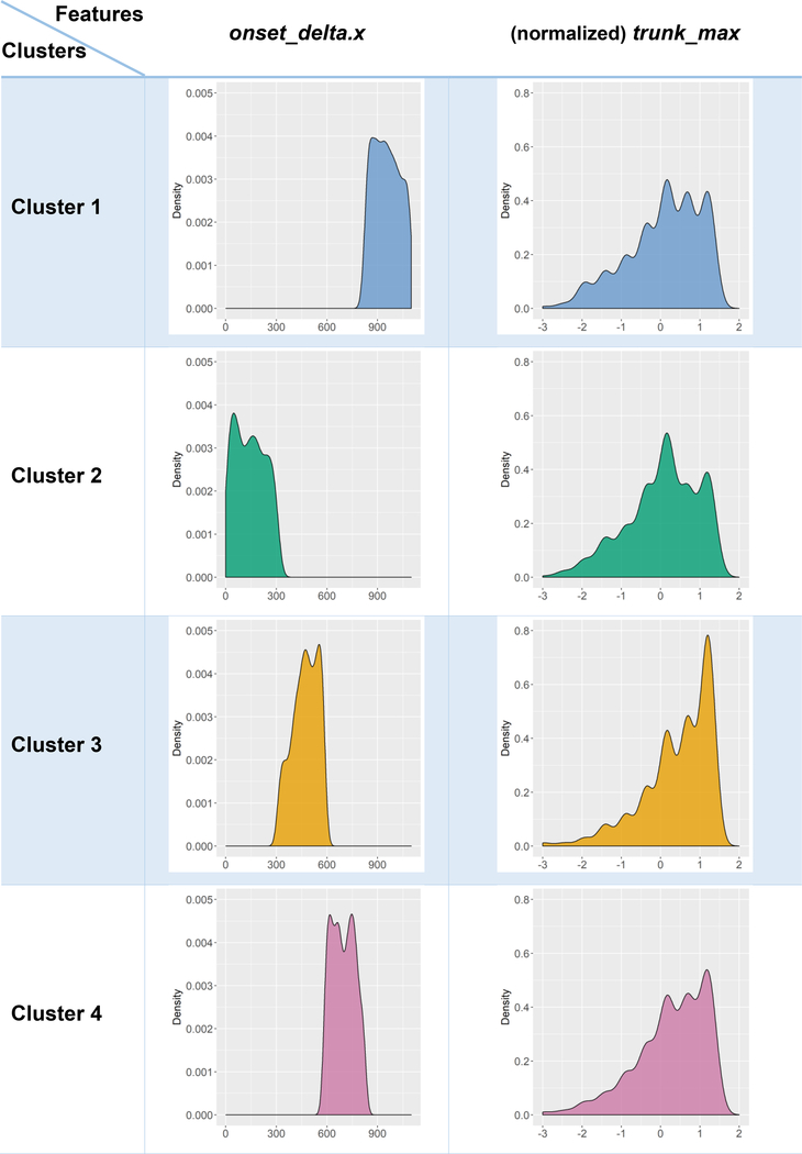
A deeper exploration of the salience of observed features as discriminants of the automatically identified computed phenotypes is illustrated on Table 8. For each pair of clusters and each observable variable, we can explicate the contrast specific distributions (for continuous) and factor-levels (for categorical) features. Demonstrating all possible scenarios is impractical, due to the number of possible combinations (of cluster pairs) and the large number of features. However, Table 8 illustrates this capability specifically for the “onset_delta.x” and “trunk_max” covariates. Graphical exploration of violin plots, box-and-whisker plots, histogram of estimated density plots provide a mechanism to examine the core univariate characteristics that segregate the derived computed phenotypes.

Table 8:

Examples of deeper exploration explicating the relation between machine-derived computed phenotypes (clusters) and observable clinical phenotypes (in terms of some ALS variables).

Dimensionality reduction using t-Distributed Stochastic Neighbor Embedding (t-SNE) [43] provided an additional confirmation of the intriguing four computable phenotypes identified independently by the unsupervised clustering. Figure 4 illustrates the flat 2D t-SNE manifold representation of the data where each case is post-hoc color-coded by its corresponding derived cluster label. The clear separation of the computed phenotypes in the t-SNE space, with only minor label overlaps, provides evidence of structure in the multivariate data recovered independently by the clustering and the t-SNE embedding methods.

Figure 4:

2D t-SNE manifold representation of the data where each case is post-hoc color-coded by its corresponding derived cluster label.

Discussion and Conclusions

Hothorn and colleagues [44] applied conditional random forests to model the trajectory of ALSFRS score over time, and their results indicated high variability of the ALSFRS ratio among the study subjects (RMSE=0.5208, Pearson correlation=0.4014). Gomeni et al. [45] used a non-linear Weibull model to describe the ALS disease progression based on ALSFRS-R, and identified two clusters of trajectories (slow progression vs fast progression) using stepwise logistic regression. Taylor and co-workers [46] selected 3,742 out of 10,700 patients, using completeness in ALSFRS-R and forced vital capacity (FVC) records, to report a random forest model outperforming other approaches in predicting 6-month ALSFRS-R score (R² = 0.582, RMSE=0.470). Ong et al. [47] found the exponential model was the best fit and categorized the subjects into fast and slow progressors based on score declined per day. Beaulieu-Jones and colleagues [48] implemented different imputation methods showing imputation does not have a significant effect on prediction. They also discovered that the progression of ALS approximately follows normal distribution.

ALS studies are complicated by the heterogeneity of this neurodegenerative disorder as well as the enormous challenges in handling, processing, and interpreting massive amounts of multi-source incongruent data serving as proxy of the onset and advancement of the disease. Providing clinical decision support to accurately prognosticate the course of the disease would be extremely valuable to identify reliable individualized predictions of the likely progression of ALS. In this study, we examined model-based (e.g., linear models) and model-free (e.g., machine-learning) methods to predict clinically relevant outcomes, e.g., change of ALSFRS score of FVC. Using independent training data (for model estimation and machine learning) and testing data (for assessing the accuracy and reliability of the predictions) we quantified the performance and compared the results of different forecasting techniques. The change of the Amyotrophic Lateral Sclerosis Functional Rating Scale (ALSFRS) slope between 3 and 12 month of monitoring was used as a diagnostic predictive outcome variable.

A 2018 postmortem study of ALS heterogeneity identified factors contributing to survival duration (0–10 years) in 800 patients [49]. Using survival regression, classification models (GML and RF), and dimensionality reduction the authors identified 38 salient measures (e.g., respiratory function, FVC, oxygen saturation, negative inspiratory force) that predicted ALSFRS-R, and other clinical outcomes. The main conclusion reported by the authors suggests that for personalized forecasting of survival, new independent metrics, as well as revisions to current metrics (e.g., ALSFRS-R), may need to be developed to capture the observed ALS heterogeneity.

Our study was based on training and testing data of patients and controls from the open Pooled Resource Open-Access ALS Clinical Trials Database (PRO-ACT) archive. The results of the study included both positive and negative findings about the impact of alternative processing protocols and the power of different analytical methods to forecast specific clinical phenotypes. The best model-based and model-free results highlight that initial measures of ALSFRS and its sub-questions most significantly contributed to the overall prediction the ALSFRS at 1 year (12-month follow up). Other variables that contributed to overall prediction included time since disease onset and various measures of hematocrit, creatinine, potassium, calcium, and alanine transaminase (ALT). The contribution of creatinine confirms some prior reports, however, in this study, uric acid was not a strong clinical predictor. That changes in ALSFRS over the initial 3 months of data collection are the most significant predictors of future ALSFRS score, which is not surprising given the curvilinear nature of this clinical measure. Our findings highlight that the ALSFRS is an informative measure, but new biologic markers are needed to improve univariate disease progression prediction and increase the reliability of such machine-learning based decision support systems. It is worth pointing out that strictly speaking, the values of each single ALSFRS item is intrinsically a discrete (ordinal/categorical) covariate. However, most studies model ALSFRS scores as continuous variables. From a methodological point of view, depending on the specific analytical strategy, treating ALSFRS as a continuous outcome may or may not be valid, e.g., classification and clustering of categorical outcomes is meaningful, but continuous regression linear modeling may be less appropriate.

Albeit direct implementations of these findings in clinical settings may still be in the future, our technique provides a roadmap for scientifically rigorous variable selection, computationally efficient inference using model-based and model-free methods, reproducible scientific discovery, and collaborative validation.

We also determined that the data preprocessing protocols may impact the results of the predictive analytics. We tried several alternative data preprocessing strategies. The main problems with preserving the bulk of the information content of the data related to data incongruency (e.g., different sampling rates) and data heterogeneity (e.g., missingness). To address the longitudinal incongruency within one covariate and one subject, we used the arithmetic average of all observed values. Initially, to handle missing values, we employed multiple imputation across all data elements and subjects. However, shot-gun approaches did not work well. This may be due to violations of the missing-at-random assumption or instability of the iterative multiple imputation algorithm on this large-scale data. Our final strategy for managing the missing data included a blended approach of (1) selective triaging of cases and variables, (2) imputing missing cells by the median value of a feature, and (3) multiple imputation on selected cases and data elements.

The Synapse ALS challenge initiative presented cluster analysis as an important approach in examining and simulating ALS disease progression. Our classification and prediction of specific univariate clinical traits were not impressive. It’s possible that better classification models can be built, estimated, and validated on larger cohorts of patients sharing similar (congruent) clinical features. Our classification attempts were not reliable in identifying specific univariate clinically-relevant outcomes. There is also little evidence of prior successful classification results in other peer-reviewed publications. However, our unsupervised clustering analysis generated highly reliable, reproducible, and consistent computable phenotypes representing four complementary sub-cohorts, which are discriminated by multivariate clinical factors. This salient phenotypic clustering based on families of clinical features may explain the observed heterogeneity of ALS morbidity.

Our investigation faced two difficult challenges. The first one was transforming and harmonizing the longitudinal data into signature vectors congruent across subjects including maximum, minimum, median and the rate. Other investigators have suggested using the “first visit”, “the last visit”, “mean” and “standard deviation” to summarize the longitudinal information. However, bringing additional per-encounter information, does not resolve the sampling incongruency. Our approach compromises between increasing the volume of preserved information and minimizing the sampling incongruency. There is some evidence that ALSFRS is not linear but curvilinear [50], however, further investigation is warranted. Another interesting prospective examination may include information about adverse events. It’s not clear if utilizing observed adverse events may improve the predictive power of the algorithms to discriminate between different ALS clinical phenotypes.

The same compromise also applies when dealing with the missing data. On the one hand, to preserve the amount of observed information, we need to keep as many features as possible. On the other hand, a large number of data elements increases the demand on the subsequent data harmonization and aggregation. Larger number of subjects included in the training and testing collections would increase the predictive power of the methods (using the training data) and improve the forecasting results (using the testing data). The strategy we used was first triaging highly missing subjects and features, followed by handling missing testing data to ensure the final training-data-derived predictors are applicable to the validation data. This homogenized the predictive features and allowed aggregation of the data that led to consistent and reliable clustering results. When some variables are highly correlated, the multiple imputation may leave a few elements as missing, e.g., when the imputation algorithm does not converge. Novel numerical methods may help to alleviate the convergence problem. Adding an observation-derived prior could shrink the covariance matrix and ease the difficulty in converging. In this study, 1% of the total observations are used for constructing the empirical prior.

This study has limitations. The PRO-ACT data contains mostly subjects that entered a clinical trial. These subjects may not reflect the true population of ALS subjects given study-specific exclusion criteria. For example, subjects with dysarthria or dysphagia or early onset respiratory insufficiency may be ineligible for a trial and may not be represented in this dataset. Nonetheless, the presented study does offer important insights into modeling complex ALS data. This is important especially when considering designing prospective ALS studies or deciding on data elements to collect in large ongoing clinical studies. Our choice to only use the original ALSFRS scores may be an additional limitation as the revised version (ALSFRS-R) includes additional assessments, e.g., dyspnea, orthopnea and ventilatory support, which could potentially provide complementary information for forecasting ALS progression or identifying ALS clinical phenotypes.

There are some reports that ALSFRS may be time sensitive [49], which would make it a tricky clinical outcome to track the longitudinal progression of ALS. Our unsupervised approach is less sensitive to the dynamics of specific clinical outcomes, as we make no assumptions on a univariate response, but rather consider all observables as time-varying predictors. In this manuscript, we did not explore specifically predicting survival duration, however, elsewhere, we have demonstrated alternative non-parametric strategies to forecast patient survival [35].

Based on the reported findings, a deductive approach examining the specific from the general may be employed to develop clinical decision support system for prospective (individualized) personalized medicine based on first understanding the (global) ALS population characteristics. Due to low signal relative to normal biological and medical variation, accurate and highly-robust predictions of ALSFRS/ALSFRS-R may not be possible using the type of data provided in the PRO-ACT archive. For instance, a Rasch-analysis of the dimensionality, reliability and validity of ALSFRS-R suggested the need for improvements of its metric quality [51]. The three factors identified by the authors included bulbar function, fine and gross motor function, and respiratory function.

Following open-science principles, we share the entire data processing protocol to enable community-wide validation, improvements, and collaborative transdisciplinary research on complex healthcare and biomedical challenges. To ensure scientific reproducibility and promote community validation of our methods and findings, the R-based ALS Predictive Analytics source-code is released under permissive LGPL license on our GitHub repository (https://github.com/SOCR/ALS_PA).

Highlights.

• Used a large ALS data archive of 8,000 patients consisting of 3 million records, including 200 clinical features tracked over 12 months.

• Employed model-based and model-free methods to predict ALSFRS changes over time, cluster patients into cohorts, and derive computable phenotypes.

• Research findings include stable, reliable, and consistent (95%) patient stratification into computable phenotypes. However, clinical explication of the results requires interpretation of multivariate information.

References

- 1.Saykin AJ, et al. , Genetic studies of quantitative MCI and AD phenotypes in ADNI: Progress, opportunities, and plans. Alzheimers & Dementia, 2015. 11(7): p. 792–814. [DOI] [PMC free article] [PubMed] [Google Scholar]
- 2.Moon SW, et al. , Structural neuroimaging genetics interactions in Alzheimer’s disease. Journal of Alzheimer’s Disease, 2015. 48(4): p. 1051–1063. [DOI] [PMC free article] [PubMed] [Google Scholar]
- 3.Moon SW, et al. , Structural Brain Changes in Early-Onset Alzheimer’s Disease Subjects Using the LONI Pipeline Environment. Journal of Neuroimaging, 2015. 25(5): p. 728–737. [DOI] [PMC free article] [PubMed] [Google Scholar]
- 4.Dinov ID, et al. , Predictive Big Data Analytics: A Study of Parkinson’s Disease Using Large, Complex, Heterogeneous, Incongruent, Multi-Source and Incomplete Observations. Plos One, 2016. 11(8). [DOI] [PMC free article] [PubMed] [Google Scholar]
- 5.Marek K, et al. , The Parkinson Progression Marker Initiative (PPMI). Progress in Neurobiology, 2011. 95(4): p. 629–635. [DOI] [PMC free article] [PubMed] [Google Scholar]
- 6.Zach N, et al. , Being PRO-ACTive: What can a Clinical Trial Database Reveal About ALS? Neurotherapeutics, 2015. 12(2): p. 417–423. [DOI] [PMC free article] [PubMed] [Google Scholar]
- 7.Atassi N, et al. , The PRO-ACT database Design, initial analyses, and predictive features. Neurology, 2014. 83(19): p. 1719–1725. [DOI] [PMC free article] [PubMed] [Google Scholar]
- 8.Dinov ID, Volume and value of big healthcare data. Journal of Medical Statistics and Informatics, 2016. 4(1): p. 1–7. [DOI] [PMC free article] [PubMed] [Google Scholar]
- 9.Chatterjee S and Hadi AS, Regression analysis by example. 2015: John Wiley & Sons. [Google Scholar]
- 10.Bergsma W, Croon MA, and Hagenaars JA, Marginal models: For dependent, clustered, and longitudinal categorical data. 2009: Springer Science & Business Media. [Google Scholar]
- 11.Markus KA, Principles and Practice of Structural Equation Modeling by Kline Rex B.. Structural Equation Modeling: A Multidisciplinary Journal, 2012. 19(3): p. 509–512. [Google Scholar]
- 12.Edwards N, Wu X, and Tseng C-W, An Unsupervised, Model-Free, Machine-Learning Combiner for Peptide Identifications from Tandem Mass Spectra. Clinical Proteomics, 2009. 5(1): p. 23–36. [Google Scholar]
- 13.Zhang GP, Neural networks for classification: a survey. IEEE Transactions on Systems, Man, and Cybernetics, Part C (Applications and Reviews), 2000. 30(4): p. 451–462. [Google Scholar]
- 14.Kai-Hsiang C, et al. , Model-free functional MRI analysis using Kohonen clustering neural network and fuzzy C-means. IEEE Transactions on Medical Imaging, 1999. 18(12): p. 1117–1128. [DOI] [PubMed] [Google Scholar]
- 15.Filzmoser P, Baumgartner R, and Moser E, A hierarchical clustering method for analyzing functional MR images. Magnetic Resonance Imaging, 1999. 17(6): p. 817–826. [DOI] [PubMed] [Google Scholar]
- 16.Witten IH and Frank E, Data Mining: Practical machine learning tools and techniques. 2005: Morgan Kaufmann. [Google Scholar]
- 17.Wistuba M, Schilling N, and Schmidt-Thieme L. Sequential Model-Free Hyperparameter Tuning. in Data Mining (ICDM), 2015 IEEE International Conference on 2015. [Google Scholar]
- 18.Saitta S, et al. , Feature Selection Using Stochastic Search: An Application to System Identification. Journal of Computing in Civil Engineering, 2010. 24(1): p. 3–10. [Google Scholar]
- 19.De Sa JM, Pattern recognition: concepts, methods and applications. 2012: Springer Science & Business Media. [Google Scholar]
- 20.Tamás Kincses Z, et al. , Model-free characterization of brain functional networks for motor sequence learning using fMRI. NeuroImage, 2008. 39(4): p. 1950–1958. [DOI] [PubMed] [Google Scholar]
- 21.Jain AK, Data clustering: 50 years beyond K-means. Pattern recognition letters, 2010. 31(8): p. 651–666. [Google Scholar]
- 22.Wismüller A, et al. , Model-free functional MRI analysis based on unsupervised clustering. Journal of Biomedical Informatics, 2004. 37(1): p. 10–18. [DOI] [PubMed] [Google Scholar]
- 23.Gong P, et al. A general iterative shrinkage and thresholding algorithm for non-convex regularized optimization problems. in International Conference on Machine Learning 2013. [PMC free article] [PubMed] [Google Scholar]
- 24.Bubeck S, Convex optimization: Algorithms and complexity. Foundations and Trends® in Machine Learning, 2015. 8(3–4): p. 231–357. [Google Scholar]
- 25.Mairal J, Incremental majorization-minimization optimization with application to large-scale machine learning. SIAM Journal on Optimization, 2015. 25(2): p. 829–855. [Google Scholar]
- 26.Fiedler M, et al. , Linear optimization problems with inexact data. 2006: Springer Science & Business Media. [Google Scholar]
- 27.Jain P and Kar P, Non-convex optimization for machine learning. Foundations and Trends® in Machine Learning, 2017. 10(3–4): p. 142–336. [Google Scholar]
- 28.Allen-Zhu Z and Hazan E. Variance reduction for faster non-convex optimization. in International Conference on Machine Learning 2016. [Google Scholar]
- 29.Kuffner R, et al. , Crowdsourced analysis of clinical trial data to predict amyotrophic lateral sclerosis progression. Nat Biotech, 2015. 33(1): p. 51–57. [DOI] [PubMed] [Google Scholar]
- 30.Zach N, et al. , Being PRO-ACTive: What can a Clinical Trial Database Reveal About ALS? Neurotherapeutics, 2015. 12(2): p. 417–423. [DOI] [PMC free article] [PubMed] [Google Scholar]
- 31.Rodriguez-Galiano V, et al. , An assessment of the effectiveness of a random forest classifier for land-cover classification. ISPRS Journal of Photogrammetry and Remote Sensing, 2012. 67: p. 93–104. [Google Scholar]
- 32.Carreiro AV, et al. , Prognostic models based on patient snapshots and time windows: Predicting disease progression to assisted ventilation in Amyotrophic Lateral Sclerosis. Journal of biomedical informatics, 2015. 58: p. 133–144. [DOI] [PubMed] [Google Scholar]
- 33.Grigull L, et al. , Diagnostic support for selected neuromuscular diseases using answer-pattern recognition and data mining techniques: a proof of concept multicenter prospective trial. BMC medical informatics and decision making, 2016. 16(1): p. 1. [DOI] [PMC free article] [PubMed] [Google Scholar]
- 34.Steinberg D and Colla P, CART: classification and regression trees. The Top Ten Algorithms in Data Mining, 2009. 9: p. 179. [Google Scholar]
- 35.Huang Z, et al. , Complete hazard ranking to analyze right-censored data: An ALS survival study. PLOS Computational Biology, 2017. 13(12): p. e1005887. [DOI] [PMC free article] [PubMed] [Google Scholar]
- 36.Ong M-L, Tan PF, and Holbrook JD, Predicting functional decline and survival in amyotrophic lateral sclerosis. PLOS ONE, 2017. 12(4): p. e0174925. [DOI] [PMC free article] [PubMed] [Google Scholar]
- 37.Westeneng H-J, et al. , Prognosis for patients with amyotrophic lateral sclerosis: development and validation of a personalised prediction model. The Lancet Neurology, 2018. 17(5): p. 423–433. [DOI] [PubMed] [Google Scholar]
- 38.Cedarbaum JM and Stambler N, Performance of the amyotrophic lateral sclerosis functional rating scale (ALSFRS) in multicenter clinical trials. Journal of the Neurological Sciences, 1997. 152: p. s1–s9. [DOI] [PubMed] [Google Scholar]
- 39.Cedarbaum JM, et al. , The ALSFRS-R: a revised ALS functional rating scale that incorporates assessments of respiratory function. Journal of the neurological sciences, 1999. 169(1): p. 13–21. [DOI] [PubMed] [Google Scholar]
- 40.Su Y-S, et al. , Multiple imputation with diagnostics (mi) in R: Opening windows into the black box. Journal of Statistical Software, 2011. 45(2): p. 1–31. [Google Scholar]
- 41.Buuren S and Groothuis-Oudshoorn K, mice: Multivariate imputation by chained equations in R. Journal of statistical software, 2011. 45(3). [Google Scholar]
- 42.Abayomi K, Gelman A, and Levy M, Diagnostics for multivariate imputations. Journal of the Royal Statistical Society: Series C (Applied Statistics), 2008. 57(3): p. 273–291. [Google Scholar]
- 43.Maaten L.v.d. and Hinton G, Visualizing data using t-SNE. Journal of machine learning research, 2008. 9(Nov): p. 2579–2605. [Google Scholar]
- 44.Hothorn T and Jung HH, RandomForest4Life: A Random Forest for predicting ALS disease progression. Amyotrophic Lateral Sclerosis and Frontotemporal Degeneration, 2014. 15(5–6): p. 444–452. [DOI] [PubMed] [Google Scholar]
- 45.Gomeni R, Fava M, and P.R.O.-A.A.C.T. Consortium, Amyotrophic lateral sclerosis disease progression model. Amyotrophic Lateral Sclerosis and Frontotemporal Degeneration, 2014. 15(1–2): p. 119–129. [DOI] [PubMed] [Google Scholar]
- 46.Taylor AA, et al. , Predicting disease progression in amyotrophic lateral sclerosis. Annals of Clinical and Translational Neurology, 2016. 3(11): p. 866–875. [DOI] [PMC free article] [PubMed] [Google Scholar]
- 47.Ong ML, Tan PF, and Holbrook JD, Predicting functional decline and survival in amyotrophic lateral sclerosis. Plos One, 2017. 12(4). [DOI] [PMC free article] [PubMed] [Google Scholar]
- 48.Beaulieu-Jones BK and Moore JH, MISSING DATA IMPUTATION IN THE ELECTRONIC HEALTH RECORD USING DEEPLY LEARNED AUTOENCODERS, in Pacific Symposium on Biocomputing 2017, Altman RB, et al. , Editors. 2017. p. 207–218. [DOI] [PMC free article] [PubMed] [Google Scholar]
- 49.Pfohl SR, et al. , Unraveling the Complexity of Amyotrophic Lateral Sclerosis Survival Prediction. Frontiers in Neuroinformatics, 2018. 12(36). [DOI] [PMC free article] [PubMed] [Google Scholar]
- 50.Gordon PH, et al. , Progression in ALS is not linear but is curvilinear. Journal of neurology, 2010. 257(10): p. 1713–1717. [DOI] [PubMed] [Google Scholar]
- 51.Franchignoni F, et al. , Evidence of multidimensionality in the ALSFRS-R Scale: a critical appraisal on its measurement properties using Rasch analysis. J Neurol Neurosurg Psychiatry, 2013. 84(12): p. 1340–1345. [DOI] [PubMed] [Google Scholar]
Associated Data
This section collects any data citations, data availability statements, or supplementary materials included in this article.