Manifold learning for parameter reduction

Abstract

Large scale dynamical systems (e.g. many nonlinear coupled differential equations) can often be summarized in terms of only a few state variables (a few equations), a trait that reduces complexity and facilitates exploration of behavioral aspects of otherwise intractable models. High model dimensionality and complexity makes symbolic, pen–and–paper model reduction tedious and impractical, a difficulty addressed by recently developed frameworks that computerize reduction. Symbolic work has the benefit, however, of identifying both reduced state variables and parameter combinations that matter most (effective parameters, “inputs”); whereas current computational reduction schemes leave the parameter reduction aspect mostly unaddressed. As the interest in mapping out and optimizing complex input–output relations keeps growing, it becomes clear that combating the curse of dimensionality also requires efficient schemes for input space exploration and reduction. Here, we explore systematic, data-driven parameter reduction by means of effective parameter identification, starting from current nonlinear manifoldlearning techniques enabling state space reduction. Our approach aspires to extend the data-driven determination of effective state variables with the data-driven discovery of effective model parameters, and thus to accelerate the exploration of high-dimensional parameter spaces associated with complex models.

1. Introduction

Our motivation lies in the work of Sethna and coworkers on model sloppiness [1], as well as in related ideas and studies on parameter non-identifiability [2], active subspaces [3] and more. These authors investigate a widespread phenomenon, in which large ranges of model parameter values (inputs) produce nearly constant model predictions (outputs). This behavior, termed sloppiness and observed in complex dynamic models over a wide range of fields, has been exploited to derive simplified models [4, 5]. Additional motivation comes from our interest in model scaling and nondimensionalization, time-honored ways to reduce complexity but often more closely resembling an art than definite algorithms.

One extreme case of sloppiness, termed parameter non-identifiability, arises when model predictions depend solely on a reduced number of parameter combinations. In such a setting, the parameter space is foliated by lower-dimensional sets along which those combinations, and hence also the resulting observables (the outputs), retain their values. In such circumstances, it is neither possible nor desirable to infer parameter values from observations; the parameters are said to be non-identifiable. One should, instead, re-parameterize the model with a reduced number of identifiable, effective parameters and, if desired, use those to explore the model input–output structure. Such identifiability analysis decomposes parameter space globally on the basis of model response, yet its symbolic nature can make it cumbersome and highly sensitive to small perturbations: even a minute dependence on certain parameter combinations can destroy the invariance of the decomposition. (Computational) sensitivity analysis is more robust, as it weighs the degree by which parameter combinations affect response; however, it is inherently not global in parameter space, as it uses a (local) linearization. We attempt to reconcile and fuse these two perspectives into an entirely data-driven, nonlinear framework for the identification of global effective parameters.

To fix ideas, we consider the caricature model of Fig. 1, given as an explicit vector function of two parameters, f₀(p₁, p₂) = (p₁p₂, ln(p₁p₂), (p₁p₂)²). Given access to input–output information (black-box function evaluation) but no formulas, one might not even suspect that only the single parameter combination p_eff = p₁p₂ matters. Fitting the model to data f* = (1, 0, 1) in the absence of such information, one would find an entire curve in parameter space that fits the observations. A data fitting algorithm based only on function evaluations could be “confused” by such behavior in declaring convergence. As seen in Fig. 1(a), different initial conditions fed to an optimizer with a practical fitting tolerance δ ≈ 10⁻³ (see figure caption for details) converge to many, widely different results tracing a level curve of p_eff. The subset of good fits is effectively 1–D; more importantly, and moving beyond the fit to this particular data, the entire parameter space is foliated by such 1–D curves (neutral sets), each composed of points indistinguishable from the model output perspective. Parameter non-identifiability is therefore a structural feature of the model, not an artifact of optimization. The appropriate, intrinsic way to describe parameter space for this problem is through the effective parameter p_eff and its level sets. Consider now the inset of Fig. 1(a), corresponding to the perturbed model f_ε(p₁, p₂) = f₀(p₁, p₂) + 2ε(p₁ – p₂, 0, 0) and fit to the same data. Here, the parameters are identifiable and the minimizer (p₁, p₂) unique: a perfect fit exists. However, the foliation observed for ε = 0 is loosely remembered in the shape of the residual level curves, and the optimizer would be comparably “confused” in practice. It is such model features that provided one of the original motivations in the work of Sethna and coworkers; in their terminology, this model is sloppy. The presence of lower-dimensional, almost neutral parameter sets (“echoed” in the elongated closed curves in the inset) increases disproportionately the importance of certain parameter combinations and reduces accordingly the number of independent, effective system parameters.

Figure 1:

Exact and learned (global) parameter space foliations for the model f_ε (p₁, p₂) = (p₁p₂ + 2ε(p₁ – p₂), ln(p₁p₂), (p₁p₂)²). The combination p_eff = p₁p₂ is an effective parameter for the unperturbed (ε = 0) model, since f₀ =const. whenever p₁p₂ =const. (a) Level sets of the cost function δ(p) = ∥f_ε (p) – f* ∥ for the unperturbed (main) and perturbed (inset) model and for data f* = (1, 0, 1) corresponding to (p₁, p₂) = (1,1). Level sets of p_eff can be learned by data fitting: feeding various initializations (triangles) to a gradient descent algorithm for the unperturbed problem yields, approximately, the hyperbola p_eff = 1 (circles; colored by initialization). This behavior persists qualitatively for ε = 0.2 despite the existence of a unique minimizer p*, because δ (p) remains within tolerance over extended almost neutral sets around p* that approximately trace the level sets of p_eff. (b) Learning p_eff by applying DMAPS, with an output-only-informed metric (see the SI), to input–output data of the unperturbed model. For ε = 0, points on any level curve of p_eff are indistinguishable for this metric, as f₀ maps them to the same output. DMAPS, applied to the depicted oval point cloud, recovers those level curves as level sets of the single leading nontrivial DMAPS eigenvector ϕ₁.

Our goal is to extract a useful intrinsic parameterization of model parameter space (input space) solely from input–output data. As we shall see, this parameterization may vary across input space regimes and, in the context of ODEs, we will associate that variation with the classical notions of regular and singular perturbations using explicit examples. For the time being, a pertinent question concerns the purely data-driven identification of the sloppy structure in Fig. 1. One answer is given by the manifold-learning technique we choose to work with in this paper: diffusion maps (DMAPS; see SI and e.g. [6]). If a given dataset in a high-dimensional, ambient Euclidean space lies on a lower-dimensional manifold, then the DMAPS objective is to parameterize it in a manner reflecting the intrinsic geometry (and thus also dimension) of this underlying manifold. In our case, we work with the space of input–output combinations, where each data point consists of parameter values and the resulting observations. DMAPS turns the dataset into a weighted graph and models a diffusion process (random walk) on it. The graph weights determine the transition probabilities between points and depend solely on an application-driven understanding of data closeness or similarity. Typically, DMAPS base this similarity measure on the Euclidean distance in the ambient space; yet, for our applications in most of this paper, this similarity will be informed solely by output observations. The dataset is parameterized, finally, by eigenvectors of the corresponding Markov matrix, relating in turn to a (discretized) eigenproblem for the Laplace–Beltrami operator on the underlying manifold [7]; one may perceive here an analogy with Singular Value Decomposition in classical Principal Component Analysis (PCA) [8]. In our input–output setting, DMAPS coordinatizes the low-dimensional manifold hosting the dataset. Both the effective parameters and the observables are now functions on this low-dimensional manifold, therefore both the input space and (what in sloppiness terminology is called) the model manifold are jointly described in terms of this intrinsic, common parameterization based on leading diffusion modes.

As a concrete example, consider randomly sampling the input space of our model above, i.e. a (p₁, p₂)–parallelogram [0, a]×[0, b] as in Fig. 1, and using as our pairwise similarity measure the Euclidean distance between points in this input space. Applying DMAPS to that dataset recovers the sampled parallelogram, i.e. DMAPS correctly identifies the dimension of the underlying manifold and coordinatizes it using two diffusion eigenmodes. For this simple shape, the leading (nontrivial, independent) eigenmodes assume the form ϕ₁(x, y) = cos(πp₁/a) and ϕ_j(x, y) = cos(πp₂/b), where the index j of the first eigenfunction independent of ϕ₁ depends on a/b. This parameterization maps the (p₁, p₂)–rectangle bijectively to the (ϕ₁, ϕ₂)–domain [−1, 1] × [−1, 1], so DMAPS recovers the original parameterization up to an invertible nonlinear transformation. Our main idea here is to retain sampling of the input (parameter) space but use, instead, a similarity measure (also) informed by the output, i.e. by the model response at the sampled parameter points. As a first but meaningful attempt for the unperturbed example above, we work with the output-only similarity measure ∥f₀(p) – f₀(p′)∥ between parameter settings p and p′. ¹

In the context of our example, the output-only similarity measure ensures that only parameter values lying on distinct level sets of p_eff are seen as distinct. Because of this, our chosen similarity measure immediately reveals the effective parameter space to be 1–D, as in Fig. 1(b). Coloring the points by the first DMAPS mode ϕ₁(p₁, p₂) confirms that this data-driven procedure “discovers” sloppiness. Data points having different parameter settings (different “genotypes”) but the same output (same “phenotypes”) are found as level sets of the first nontrivial DMAPS eigenfunction ϕ₁ on the dataset, obtained in turn by our black-box simulator and without recourse to the explicit input–output relation f₀. Additionally, the decomposition of parameter space into “meaningful” and “neutral” parameter combinations can be performed using a small local sample, possibly resulting from a short local search – e.g. a few gradient descent steps, or local brief simulated annealing runs. This type of local decomposition can prove valuable to the optimization algorithm, as it reveals local directions that are fruitful to explore and others (along neutral sets) that preserve model predictions (goodness of fit). These latter ones may, in turn, become useful later in multi-objective optimization, where one optimizes additional objectives along level sets discovered during optimization of the original one [10]. It is precisely the preimages, in parameter space, of the level sets of the first meaningful DMAPS coordinate ϕ₁ that correspond to the neutral parameter foliation.

The remainder of the paper is structured as follows: In Section 2, we use a simple, linear, 2–D, singularly perturbed dynamical system to bring forth the components of our data-driven framework, while retaining the connection with sloppiness terminology. Readers unfamiliar with DMAPS may want to start with the brief relevant material in the SI. The main result we illustrate in that section is the connection between singular perturbation dynamic phenomenology and data-driven detection of (what one might consider as) loss of observed dimensionality. This occurs here simultaneously in both state (model output) and parameter (model input) space. We also explore the transition region between unperturbed and singularly perturbed regimes and, finally, contrast “data-driven singular perturbation detection” with “data-driven regular perturbation detection” through another simple–yet informative–caricature. In Section 3, we move beyond caricatures to other prototypes. In Section 3a, we explore a simple kinetic example with two sloppy and one meaningful nonlinear parameter combination, readily discovered by DMAPS. This brings up the important issue of physical understanding: the correspondence between input combinations uncovered through data mining and physically meaningful parameters. That model also enables comparison of analytical and data-driven approaches (QSSA, [11]). Section 3b uses the time-honored, textbook example of Michaelis–Menten–Henri enzyme kinetics to show something we found surprising: how data-driven computations may discover parameter scalings (in this case, an alternative nondimensionalization) that better characterize the boundaries of the singular perturbation regime. Section 3 concludes with the discussion of an important subject, namely non-invertible input–output relations. We elucidate that issue using a classical chemical reaction engineering literature example, connecting the Thiele modulus (parameter) and the effectiveness factor (model output) for transport and reaction in a catalyst pellet. An important connection between the dynamics of our measurement process and our data-mining framework arises naturally in this context. In Section 4 we summarize, and also bring up analogies with and differences from the active subspace literature: the “effective parameters” discovered by DMAPS are nonlinear generalizations of linear active subspaces. We conclude with a discussion of shortcomings, as well as possible extensions and enhancements of our approach.

2. Singularly/Regularly Perturbed Prototypes

To fix ideas and definitions, we start with a dynamical model

$$\stackrel{.}{\mathbf{x}}(t\mid \mathbf{p})=\mathbf{v}(\mathbf{x}\mid \mathbf{p})\text{and}\mathbf{x}(t_0\mid \mathbf{p})={\mathbf{x}}_0(\mathbf{p}),\text{where}\stackrel{.}{\mathbf{x}}\equiv \frac{d\mathbf{x}}{\mathit{dt}}.$$ (1)

The vector $\mathbf{x}(t\mid \mathbf{p})\in {\mathbb{R}}^d$ collects the state variables at time t that are observed for parameter settings $\mathbf{p}\in {\mathbb{R}}^M$, initialization x₀(p) at t₀ and vector-field $\mathbf{v}(\cdot \mid \mathbf{p}):{\mathbb{R}}^d\to {\mathbb{R}}^d$ Equation (1) determines the system state x(t∣p) for all times t > t₀, but the model output or response consists only of partial observations of that time course; e.g. certain state variables at specific times. Observing the system means fixing p and initial conditions (inputs) and recording a number N ≥ M of scalar outputs into $\mathbf{f}(\mathbf{p})\in {\mathbb{R}}^N$. Each input yields a well-defined output f (p); as the former moves in parameter space, the latter traces out a (generically M–dimensional) model manifold $\mathcal{M}$. Our data points on this manifold are input–output combinations $(\mathbf{p},\mathbf{f}(\mathbf{p}))\in {\mathbb{R}}^{M+N}$ and not merely the outputs; see SI. In the interest of visualization, whenever the map p ↦ f (p) is injective below, we only plot the projection of the model manifold on the output space ${\mathbb{R}}^N$. To illustrate these definitions, we consider a singularly perturbed caricature chosen for its amenability to analysis,

$$\begin{array}{c}\stackrel{.}{x}=2-x-y,\hfill \\ \epsilon \stackrel{.}{y}=x-y,\hfill \end{array}\text{with}\begin{array}{c}x(0)=x_0,\hfill \\ y(0)=y_0.\hfill \end{array}$$ (2)

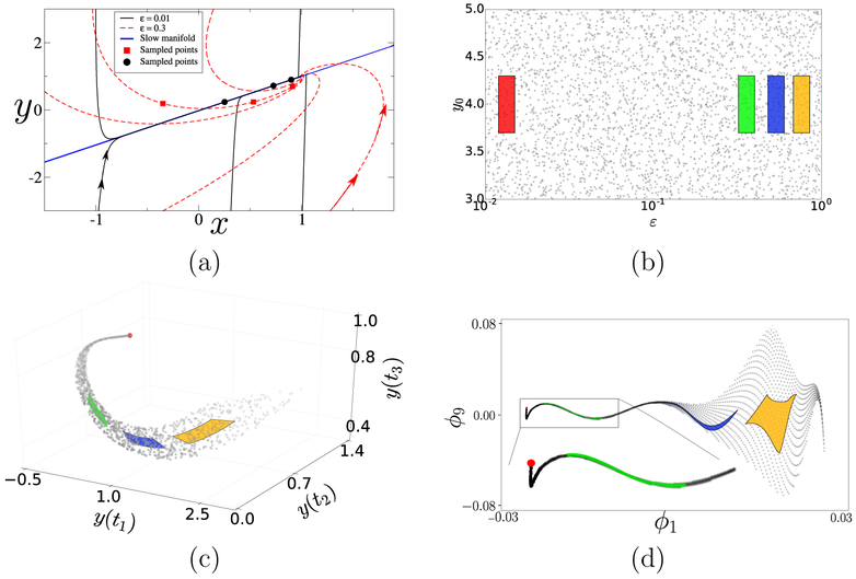
We also fix x₀ and distinct times t₁, t₂, t₃ (see caption of Fig. 2), view both p = (ε, y₀) as inputs and monitor y; concisely, f (p) = [y(t₁∣_p), y(t₂∣p), y(t₃∣p)]. The final ingredient is a metric that provides the DMAPS kernel with a measure of closeness between different input–output combinations. For simplicity, we discuss here the output-only Euclidean metric ∥f (p) – f (p′)∥ and defer a discussion of other options to a later section. The phase portraits corresponding to two distinct ε–values are plotted in Fig. 2(a). For small enough ε, all points on the vertical line segment x = x₀ (fast fiber) contract quickly to effectively the same base-point on a 1–D invariant subspace (slow subspace) before our monitoring even begins. Memory of y₀ and of the boundary layer (inner solution) is practically lost and, in the timescale of our monitoring protocol, trajectories with bounded y₀ shadow the evolution of that base-point and yield, with $\mathcal{O}(\epsilon )$ accuracy, the same output mirroring the leading order slow dynamics (outer solution). As ε increases, the output begins to vary appreciably because the fast contraction rate decelerates and the slow invariant subspace is perturbed. However, observations still lie practically on the slow subspace and are thus insensitive to y₀. For even larger ε, the disparity in contraction rates is relatively mild and different inputs yield visibly different trajectories; the output is jointly affected by ε and y₀.

Figure 2:

(a) Phase portrait of (2) for a range of initial conditions (x₀, y₀) and two representative ε–values. Solid points mark states at the monitoring times (t₁, t₂, t₃) = (0.5, 1, 1.5) for trajectories starting at x₀ = −1. For ε = 0.01, the points lie close to the slow subspace and appear y₀–independent; for ε = 0.3, instead, they lie off it and vary appreciably with y₀. (b) A sample of the model input space, overlaid with distinct rectangular patches. (c) Mapping of the input sample of panel (b) to the 3–D output space. The images of the random sample outline part of the model manifold, while those of the patches show the dimensionality reduction due to the singularly perturbed structure of the model. (d) Mapping of the input sample in DMAPS coordinates. The transformations from (b) to (c–d) are discussed in the text.

This situation is evident in Fig. 2(b–c), showing a randomly sampled set of inputs p⁽¹⁾, … , p^(L) and their simulated outputs f (p⁽¹⁾), … , f (p^(L)); the colored patches are meant as visual aids. The yellow patch outside the singularly perturbed regime maps into a 2–D region of the model manifold, whereas intermediate ones (blue, green) are gradually stretched into 1–D segments; as ε ↓ 0, or log(ε) → – ∞, the effective model manifold dimensionality cascades from two to one to zero. In the 1–D part of the model manifold and over the scales we consider, ε informs model output much more strongly than y₀. As ε ↓ 0, the output trajectory approaches a well-defined limit – the leading order outer solution – and all inputs are mapped to within $\mathcal{O}(\epsilon )$ of a parameter-free output: the model manifold “tip.” This is evident in the red patch deep inside the singularly perturbed regime, demonstrating the joint reduction in state and in parameter space dimensionality for the scales of interest: first, the evolution law involves a single state variable, with the other slaved to it algebraically; and second, all small enough ε–values produce at leading order the same, practically y₀–independent output.

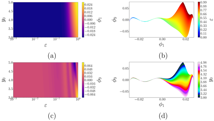
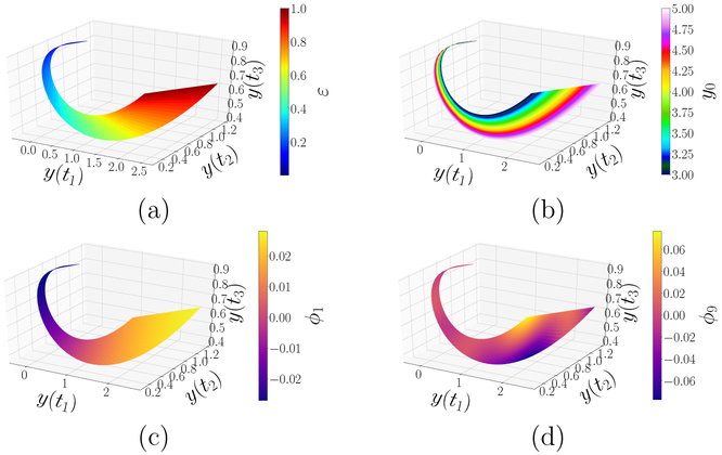
To glean the information above by data mining, we apply DMAPS (see [12] for the code) with an output-only informed kernel to the dataset and obtain the re-coordinatization $({\mathbf{p}}^{(\ell )},\mathbf{f}({\mathbf{p}}^{(\ell )}))\mapsto ({\varphi }_1^{(\ell )},{\varphi }_9^{(\ell )})$. Here, ${\varphi }_1,{\varphi }_9\in {\mathbb{R}}^L$ are independent eigenvectors of the DMAPS kernel, i.e. discretizations (on the dataset) of eigenfunctions of the Laplace–Beltrami operator defined on the model manifold $\mathcal{M}$. As such, they describe diffusive eigenmodes whose level sets endow $\mathcal{M}$ with an intrinsic, nonlinear coordinate system. The domain of that coordinate system (DMAPS space) is shown in Fig. 2(d). Here also, the stretching factor increases and the dimensionality of the mapped patches cascades, as we progress into the singularly perturbed regime. The preimage, in parameter space, of that coordinate system is shown in Fig. 3(a,c), allowing us to define distances between inputs in terms of the outputs they generate. Figure 3(b,d) portrays complementary images, namely the coordinatization of DMAPS space in terms of the inputs ε and y₀. Finally, Fig. 4(a–b) and Fig. 4(c–d) show the model manifold colored by the inputs as well as by the diffusion eigenmodes.

Figure 3:

Application of DMAPS to the singularly perturbed model (2) with an output-only-informed metric. (a, c) Input (parameter) space, coordinatized by two independent eigenmodes ϕ₁ and ϕ₉; (b,d) the diffusion coordinate domain (DMAPS space), coordinatized by ε and y₀. All parameter settings in the singularly perturbed regime (ε ⪅ 0.03) yield effectively the same model response, (ϕ₁, ϕ₉) ≈ (−0.028, 0) in diffusion coordinates, as seen by the broad monochromatic swaths at small ε–values in (a,c). Intermediate ε–values (0.03 ⪅ ε ⪅ 0.2) yield an effectively 1–D output: ϕ₉ becomes slaved to ϕ₁, see (b,d). Even larger ε–values yield a fully 2–D model manifold, captured by the independent color variation in all panels. The progressive decline of effective domain dimensionality is evident, as ε decreases, as is the loss of memory of the initial condition y₀, starting already in the 1–D regime.

Figure 4:

(a–b) Model manifold colored by the model parameters (inputs). For large ε, the model manifold is evidently coordinatized by (ε, y₀). As ε decreases, the system loses memory of the initialization y₀ and model responses for different y₀ bundle together. In the singularly perturbed regime (deep blue in panel (a)), all memory of y₀ has been lost. (c–d) Model manifold colored by leading independent DMAPS coordinates. Evidently, ϕ₁ tracks ε well, with the regime ε ≪ 1 corresponding to ϕ₁ ≈ −0.028. The coordinate ϕ₉ is transverse to ϕ₁ in the 2–D regime but, as ε decreases, becomes slaved to it and dimension reduction occurs.

These figures relate input, output and DMAPS domains to model dynamics and suffice to reproduce our earlier observations on model output. In the 2–D part of the DMAPS domain and of the model manifold, distinct points on the latter correspond to distinct diffusion coordinates and distinct inputs ε and y₀; see Fig. 3. As ε decreases, however, the dependence on y₀ becomes attenuated and the output controlled by ε alone. In the terminology introduced earlier, y₀ becomes sloppy and both the DMAPS domain and the model manifold transition to a 1–D regime parameterized by ε; the y₀–values span an ever-diminishing width. In this regime, the level sets of the eigenmodes visibly align with each other, both in input space and on the model manifold; see Fig. 3(a,c) and Fig. 4(c–d). Finally, as ε ↓ 0, all parameter settings converge to the same (ϕ₁, ϕ₉)–value, as the output converges to the “tip” of the model manifold and of the DMAPS domain.

In summary, our output-informed application of DMAPS parameterizes the input–output combinations comprising the dataset in a manner indicative of how model inputs dictate model outputs. The parameterization applies primarily to the output component of the dataset, but it can be pulled back to yield a simultaneous, consistent re-parameterization of the input component. This showcases the main contribution in this paper: a way to intuit system properties by parameterizing the input–output relation through the geometry of the manifold that collects model inputs and model outputs, as encoded in eigenfunctions of the Laplace–Beltrami operator.

2.1. Regularly perturbed prototype

In the singularly perturbed prototype discussed above, we noted the simultaneous loss of output sensitivity to (certain) initial conditions and parameters, as ε ↓ 0. Additionally, we demonstrated how this system behavior can be intuited by mining input–output data with the help of DMAPS. Figure 5(b) shows the result of applying the same methodology to the regularly perturbed example

$$\stackrel{.}{x}=-x+\epsilon x^3,\text{with}x(0)=x_0.$$ (3)

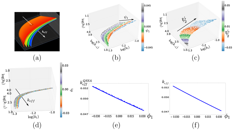
Figure 6:

Data-driven detection and characterization of the effective parameter k_eff for (4) using DMAPS. All datasets were obtained by presetting the reference output f* = f (p*) with p* = (10⁻¹, 10³, 10³) and a specific tolerance δ > 0 and, then, sampling log-uniformly a rectangular domain in input space to retain inputs satisfying ∥f (p) – f*∥ < δ. (a) Illustration of level sets of k_eff in parameter space (k₁, k₋₁, k₂). Equation 6 dictates that points on each same colored foil exhibit nearly identical model responses. (b–c) Dataset for δ = 0.001; this is practically the 2–D surface k_eff (p) = k_eff (p*) of (almost) perfect fits. An application of input-only DMAPS on this set reveals its 2–D nature and coordinatizes it through the eigenfunctions ψ₁, ψ₂. (d) Dataset for δ = 0.1, colored by the first output-only DMAPS eigenfunction ϕ₁. DMAPS clearly discovers the effective parameter, as ϕ₁ remains effectively constant on level sets of k_eff. This striking one-to-one relation is evident in panel (f), in terms of the (ϕ₁, k_eff)–coordinates. The same dataset plotted in (ϕ₁, $k_{\text{eff}}^{\text{QSSA}}$–coordinates (panel e) is, by contrast, visibly noisier.

Here also, we view p = (ε, x₀) as parameters and monitor the system state x(t∣p) at distinct times.

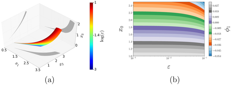
Similarly to the singularly perturbed model, the model output approaches a well-defined, limiting response in the asymptotic regime ε ↓ 0. Yet, in this case that response remains strongly dependent on x₀: distinct initial conditions yield distinct outputs even for ε ↓ 0, as seen plainly in Fig. 5. In panel (a), the limiting edge ε = 0.001 is seen to outline a 1–D boundary of the full 2–D model manifold, instead of a point as was the case for the singularly perturbed model. That same edge is seen to be parameterized by ϕ₁, in panel (b), rather than correspond to a single ϕ₁–value. This result is clearly underpinned by the uniform convergence of the trajectory x(t∣p) to x(t∣0, x₀) = x₀e^–t, which is ε–free but depends strongly on x₀ and defines the aforementioned 1–D model manifold boundary. This regular perturbation behavior, and specifically the lack of dimensionality reduction in terms of initial conditions, generalizes directly to higher state and parameter space dimensions.

Figure 5:

Model manifold and parameter space for the regularly perturbed system (3) with inputs (ε, x₀) and monitoring times (t₁, t₂, t₃) = (0.25, 1.0, 1.75). (a) Model manifold colored by ε and its projections on the coordinate planes. For large ε, the system is fully 2–D (orange/red region). As ε decreases, the model response becomes increasingly determined by x₀ alone. Contrary to Fig. 3, where the ε ≪ 1 regime was mapped to a limiting point, the limiting submanifold here is 1–D (blue straight line). (b) Parameter space colored by the DMAPS coordinate ϕ₁. DMAPS visibly captures the importance of x₀, as ε ↓ 0: the parameterization varies in the x₀ direction and remains unchanged along lines of constant x₀.

3. Beyond caricatures

3.1. The ABC model

Having examined simple singularly and regularly perturbed models, we turn our attention to the data-driven detection of an effective parameter in a paradigmatic chemical reaction network. We specifically consider the three-species, analytically tractable system (SI)

$$\mathrm{A}\underset{k_{-1}}{\overset{k_1}{\rightleftharpoons }}\mathrm{B}\stackrel{k_2}{\to }\mathrm{C},\text{initialized with}{A}_0=1,B_0=C_0=0.$$ (4)

The Quasi-Steady-State Approximation (QSSA; [13, Ch. 5]) for mechanism (4)

$$C(t\mid \mathbf{p})=1-e^{-k_{\text{eff}}^{\text{QSSA}}t},\text{where}{k}_{\text{eff}}^{\text{QSSA}}=\frac{k_1{k}_2}{(k_{-1}+k_2)},$$ (5)

and is valid for k₁ ↓ k₂ [13]. A detailed analysis, however (see SI), establishes that the approximate solution is actually

$$C(t\mid \mathbf{p})=1-e^{-k_{\text{eff}}t},\text{where}{k}_{\text{eff}}=\frac{k_1{k}_2}{k_{-1}+k_1+k_2}.$$ (6)

To detect this dimensionality reduction and “discover” k_eff in a data-driven manner, we view the kinetic constants as inputs, p = (k₁, k₋₁, k₂), and monitor product concentration at preset times, f (p) = [C(t₁∣p), … , C(t₅∣p)]. Then, we fix a model output in the regime of applicability of (6) and mine sampled parameter settings with outputs “similar” to that reference response. Here, we used as reference the output corresponding to parameter settings p* = (10⁻¹, 10³, 10³) and measured similarity in the Euclidean sense, retaining sampled points p satisfying ∥f (p) – f (p*)∥ < δ for some δ > 0. Figure 6(b–f) examines two nested such “good datasets”, one of almost perfect fits (δ = 10⁻³; Fig. 6(b-c)) and another of less good fits (δ = 10⁻¹; Fig. 6(d)). Data-mining the “zero residual level set” in 3-D parameter space with an input-only informed DMAP metric confirms its 2-D nature. The data-driven coordinatization of the full input space by output-only ϕ₁ and input-only (ψ₁, ψ₂) decomposes the space in a manner tuned to model output. A related data-processing of good fits using linear PCA was performed, e.g., as in [14] for a neuron model; clearly, linear PCA here would give the erroneous impression of full-dimensionality due to manifold curvature.

This result is valid in the input regime k₁k₂ ≪ (k₁ + k₋₁ + k₂)², that extends the QSSA, and k_eff is the effective parameter (approximately) determining the output. This expression represents a reduction of input space from 3–D to 1–D; the foliation of parameter space by the (nonlinear) level sets of k_eff is shown schematically in Fig. 6(a). The set of parameter settings with outputs within δ = 10⁻¹ of the reference output is clearly 3–D and visibly composed of level sets of k_eff spanning an appreciable k_eff range. An application of DMAPS with the Euclidean, output-only-informed similarity measure reveals the existence of a single effective parameter without recourse to an analytic expression. Indeed, the DMAPS coordinate ϕ₁ traces k_eff accurately, see Fig. 6(d,f). Note, for comparison, that $k_{\text{eff}}^{\text{QSSA}}$ is a worse predictor of model output, see Fig. 6(e). It follows that level sets of ϕ₁ in parameter space give (almost) neutral sets, i.e. level sets of k_eff whose points yield indistinguishable outputs. An algorithm to explore parameter space effectively would march along ϕ₁, whereas sampling parameter inputs at constant ϕ₁ would allow one to map out level sets of k_eff. This can be of particular utility in multi-objective optimization [10], where a second objective can be optimized on the set k_eff = k_eff (p*) optimally fitting the data f* = f (p*).

Fig. 6(e,f) raises the crucial issue of physical interpretation of the effective parameters discovered through data mining. Although such data-driven parameters are not expected to be physically meaningful, the user can postprocess their discovery by formulating and testing hypotheses on whether they are one-to-one with (i.e., encode the same information as) physically meaningful parameters.

3.2. Michaelis–Menten–Henri (MMH)

Continuing the development of a data-driven framework to identify effective parameters, we now treat a benchmark for model reduction methods. The MMH system [15, 16] describes conversion of a substrate S into a product P through mediation of an enzyme E and formation of an intermediate complex C,

$$\mathrm{S}+\mathrm{E}\underset{k_{-1}}{\overset{k_1}{\rightleftharpoons }}\mathrm{C}\stackrel{k_2}{\to }\mathrm{P}+\mathrm{E}.$$

Under conditions often encountered in practice, the first reaction step reaches quickly an (approximate) chemical equilibrium and becomes rate-limiting. Product sequestration proceeds on a much slower timescale, during which the first reaction approximately maintains its quasi-steady state.

In that regime, simultaneous state and parameter space reduction is possible, as system evolution is described by a single ODE involving a subset of the problem parameters. There have been several, increasingly elaborate estimates of the parametric regime where QSSA applies, which were underpinned by different system nondimensionalizations. The first key estimate was that of [17], where the authors identified that regime as E_T ≪ S_T involving the (conserved) total amounts of enzyme, E_T = E + C, and substrate, S_T = S + C + P. In that regime, nearly all enzyme molecules become quickly bound to substrate and the complex saturates. The authors of [18] brought the kinetic constants into play and extended the regime to E_T ≪ S_T + K_M, where K_M = (k₋₁ + k₂)/k₁ is the so-called Michaelis–Menten constant. This asymptotic regime extends the one of [17] by including the case where the complex dissociates much faster than it forms.

Our goal in this section is twofold: first, to identify the effective parameterS) informing system evolution in the asymptotic regime; and second, to show how the extended parametric region of [18] is captured in a data-driven manner by our methodology. To accomplish this in a completely automated way would necessitate using a black-box simulator for (a subset of) the dimensional state variables S, E, C, P evolving in dimensional time T. This, in turn, would necessitate a candid discussion on tuning of monitoring times to capture the slow dynamics and how that relates to experimental/simulation data. We circumvent this issue here for brevity and focus, instead, on the equivalent, non-dimensional version in [18]. In that version, T, S, C, E, P have been rescaled into dimensionless variables t, s, e, c, p; additionally, e, p have been eliminated using the enzyme and substrate conservation laws. The result is the 2–D ODE system

$$\begin{gathered} \stackrel{.}{s}=(\kappa +1)[-(1+\sigma )s+\sigma \mathit{cs}+\kappa {(\kappa +1)}^{-1}c], \\ \epsilon \stackrel{.}{c}=(\kappa +1)[(1+\sigma )s-\sigma \mathit{cs}-c]. \end{gathered}$$ (7)

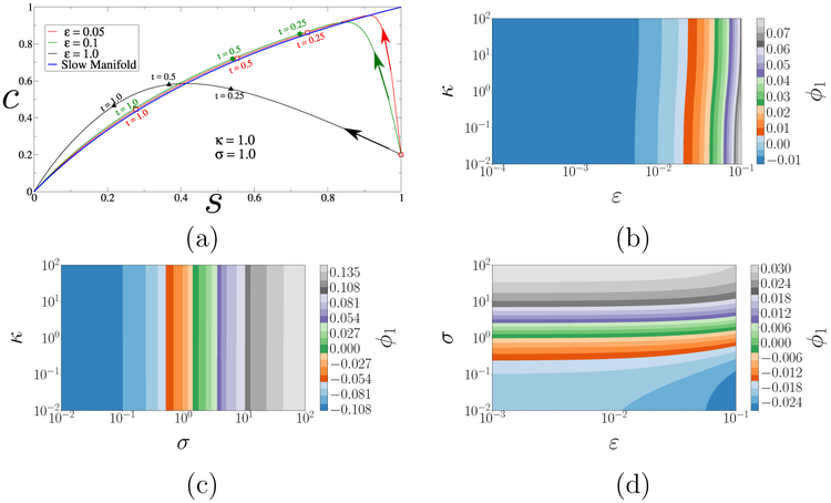
The composite parameters here are ε = E_T/(S_T + K_M), σ = S_T/K_M and κ = k₋₁/k₂, and they may in principle assume any positive value. The initial conditions (s₀, c₀) are arbitrary, and e, p can be recovered from the rescaled conservation laws e + σc/(σ + 1) = 1 and s + εc + p = 1. The system is expressed in slow time, so that quasi-steady state is achieved over an $\mathcal{O}(\epsilon )$ time and product sequestration occurs over an $\mathcal{O}(1)$ timescale. In this reformulation, the asymptotic regime where QSSA applies is ε ≪ 1, according to [18], and ε_h = (1 + 1/σ) ε ≪ 1 according to [17]; the former plainly extends the latter. Initially, we select as our observable the rescaled complex concentration at distinct times (t₁, t₂, t₃) = (0.5, 1, 1.5), so f (p) = [c(t₁∣p), c(t₂∣p), c(t₃∣p)]^T Our parameter set is the triplet p = (ε, σ, κ), with (s₀, c₀) = (1, 0) fixed as in the original experimental setting [16].

Figure 7(b–d) demonstrates that the model response is unaffected by κ and strongly affected by σ, with the limit ε ↓ 0 corresponding to an asymptotic regime. Further, Fig. 7(d) makes it plain that the system evolution in that regime is controlled by σ. This is in stark contrast to the parameter-free reduced dynamics of caricature (2) and agrees with theory, which predicts that the evolution of p in $\mathcal{O}(1)$ timescales is dictated by the leading order problem [18] (see also SI).

Figure 7:

(a) Phase portrait of the rescaled MMH model (7) with σ = κ = 1. The plotted trajectories start at (1, 0.2) and correspond to various ε–values, to illustrate the rate of attraction to the slow manifold (blue) and subsequent convergence to the origin. (b–d) Parameterization of the facets σ = 1, ε = 0.1 and κ = 10 of the (ε, σ, κ)–space (input space) by the leading (output-only) DMAPS eigenvector ϕ₁. Evidently, κ is sloppy: the output is insensitive to it over several orders of magnitude. As ε ↓ 0, the system enters an asymptotic regime whose slow, reduced dynamics is strongly informed solely by σ.

$$p=1-s-\epsilon c,\text{subject to}\stackrel{.}{s}=-c=-(1+1∕\sigma )\frac{s}{s+1∕\sigma }.$$ (8)

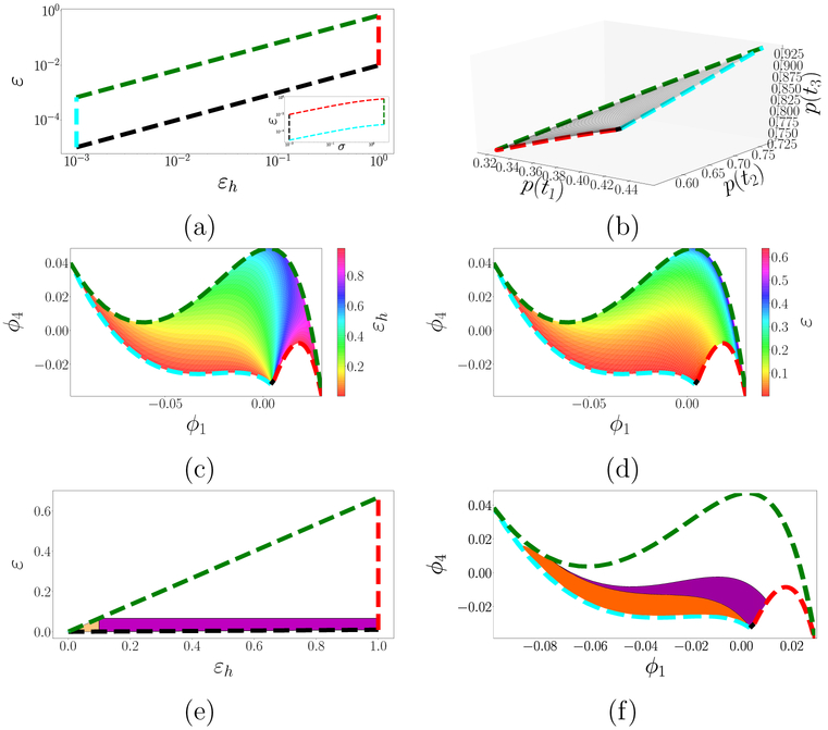
On the basis of these results, we conclude that the model manifold is effectively 2–D and not 3–D as one might initially surmise, with the asymptotic regime ε ↓ 0 corresponding to a curve parameterized only by σ. As a corollary, the model manifold dimensionality transitions from two to one in that regime, without being further reduced to zero. This is evident in Fig. 8(b), showing (part of) the model manifold for the setup above.

Figure 8:

(a) Relevant parameter domains in (ε_h, ε)-space and in (σ, ε)–space (inset; both logarithmic), related through σ = 1/(ε_h/ε – 1). Boundaries are colored consistently across panels to help visualize the transformations between spaces. (b) Model manifold $\mathcal{M}$ in output space, as (ε_h, ε) vary and κ = 10 is fixed. (c–d) Model manifold observed in DMAPS space, colored by ε_h in panel (c) and by ε in panel (d). (e) Similar to (a) but with uniform (not logarithmic) spacing, and with the highlighted regions ε_h ≪ 1 (orange triangle) and ε ≪ 1 (orange triangle and purple rectangle). (f) Image of the regions highlighted in panel (e) in DMAPS space.

We next turn to a data-driven characterization of the asymptotic regime and relate that to the characterizations in [17, 18]. Using simulated trajectories of (7) and applying our DMAP methodology with an output-only informed metric, we coordinatize the model manifold through the independent eigenmodes (ϕ₁, ϕ₄). Figures 8(c–d) show that manifold in DMAPS space; the asymptotic limit is the lower-left bounding curve (light blue). We can use these diffusion coordinates to characterize the asymptotic regime as a neighborhood of that boundary, so that the success of ε_h and ε in capturing that regime is measured by the extent their level sets track the boundary. Figures 8(c–d) color the DMAPS domain by ε_h and by ε; plainly, the ε–coloring traces the domain boundary quite well, with ε ≪ 1 represents a bona fide neighborhood of it. Small values of ε_h, on the other hand, fail to outline such a neighborhood: all level sets coalesce at the single point representing the ε_h–axis (i.e. the regime σ ↓ 0). This is made even plainer in Fig. 8(e–f), where one sees how the ε_h ≪ 1 regime misses a substantial part (colored purple) of the asymptotic regime captured by ε ≪ 1. On account of this, we can conclude that ε is indeed a better “small parameter” than ε_h. It is important to note that a black-box, data-driven approach can have no knowledge of ε, ε_h or any other “human” description of the problem. What it can do, as we just saw, is enable us to test human-generated hypotheses on the data; we – or Segel and Slemrod [18] – are the ones generating the hypotheses.

4. Non-invertible input-output relations

Throughout this paper so far, we have used an output-only-informed kernel to obtain intrinsic DMAPS parameterizations of the combined input–output manifold. Our approach consisted of using eigenfunctions of the Laplace–Beltrami operator on the model manifold, and our insights about parameter (input) space came from how it was jointly parametrized by these eigenfunctions. The approach was useful in the data-driven study of parameter non-identifiability and even sloppiness. We will now show that it fails dramatically when the mapping from parameter space to the model manifold is noninvertible, i.e. when distinct, isolated parameter values produce identical model responses, f (p) = f (p′) for p ≠ p′.

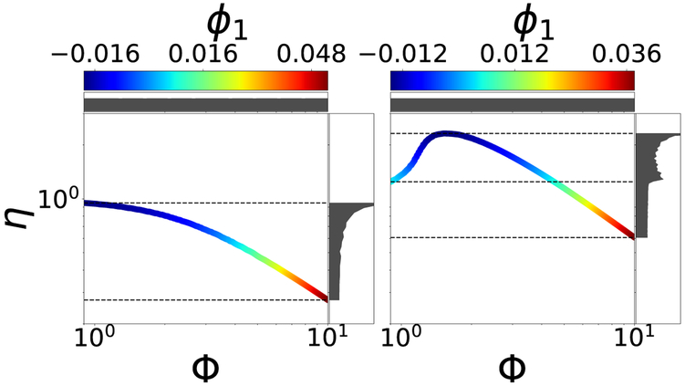
A well-known instance of this situation arises in the study of reaction–diffusion in porous catalysts and is illustrated in Fig. 9. For isothermal reactions, the output – the dimensionless “effectiveness factor” f (p) ≡ η – is a monotonic function (with known asymptotic limits) of the input – the Thiele modulus p ≡ Φ [19] (Fig. 9, left). For exothermic reactions, however, η may depend on Φ nonmonotonically and the relation becomes noninvertible; alternatively, points on the model manifold are revisited, as the input sweeps the positive real axis, Fig. 9 (right). Sampling the input Φ uniformly on the horizontal axis naturally results in a nonuniform density for the output η on the vertical axis (plotted on the right of each panel in Fig. 9). This observed output probability density function (pdf) embodies the input-output relation and brings to mind an analogy with Bayesian measure transport from a prior density to a posterior one. It is worth noting that, noninvertibility causes pronounced discontinuities on the output pdf on the right.

Figure 9:

Left: Output η, vs. input Φ for the isothermal catalyst pellet (β = 0.0, see SI) colored by ϕ₁. Right: Same plot for a nonisothermal (β = 0.2) pellet. For uniform input Φ sampling, the observed output pdf’s (see text) are plotted alongside each panel. Using output-only informed DMAPS is unable, as the coloring shows, to accurately parameterize the noninvertible case: Widely different sections of the curve on the right take on the same color. Note also the discontinuity in the density along the η axis in the right figure, a hallmark of noninvertibility.

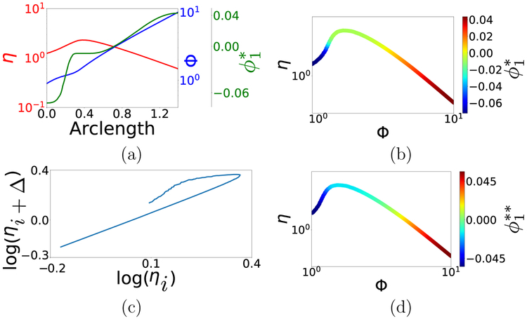
Coloring input–output (η – Φ) profiles by the leading DMAPS eigenfunction of an output-only-informed kernel shows that the data-driven coordinate, ϕ₁, which successfully recovered (parameterized) the input Φ on the left fails to do so on the right. The problem lies with the output-only metric employed, and its resolution requires a new, more informative DMAPS kernel such as

$$K^{\ast }(\mathbf{p},{\mathbf{p}}^{\prime })=\text{exp}\left(-\frac{{\Vert \mathbf{p}-{\mathbf{p}}^{\prime }\Vert }^2}{{ϵ}^2}-\frac{{\Vert \mathbf{f}(\mathbf{p})-\mathbf{f}({\mathbf{p}}^{\prime })\Vert }^2}{{ϵ}^a}\right).$$ (9)

Taking into account both inputs (p – p′) and outputs (f (p) – f (p′)), this kernel manages to differentiate inputs having the same output. Figure 10(b) corroborates the appropriateness of this kernel for a = 4: its primary eigenvector varies monotonically over the model manifold. This is also evident in Fig. 10(a), in which we have plotted input, output and the data-driven parameter ${\varphi }_1^{\ast }$ against arclength of the input–output response curve. In effect, ${\varphi }_1^{\ast }$ is in an one-to-one correspondence with the arclength, and thus “discovers” a good parameterization of the curve. This particular (a = 4) kernel – originally proposed by Lafon [7] in a different context – prioritizes output over input; due to the ϵ–scalings, the input-term only becomes significant when needed, i.e. for nearby inputs producing similar outputs.

Figure 10:

(a) Input Φ, output η and DMAPS eigenfunction ${\varphi }_1^{\ast }$ corresponding to (9) plotted against the arclength of the curve in Fig. 9. The eigenfunction clearly parameterizes both input and output. (b) input–output response curve colored by the eigenfunction ${\varphi }_1^{\ast }$ using (9) with ϵ = 0.0125. In both (b) and (c), Φ was sampled on a uniform grid between 0.9 and 10 for a total of 1043 points. (c) Plot of log(η_i+Δ) (corresponding to log(Φ_i) + Δ where Δ ≈ 0.05.) against log(η_i) (corresponding to log(Φ_i)); this “delay embedding” is one-to-one with the original curve. (d) input–output response curve colored by the eigenfunction ${\varphi }_1^{\ast \ast }$ corresponding to the “augmented output” DMAPS kernel $K^{\ast \ast }\equiv \text{exp}(-{(\stackrel{‒}{\eta }-{\stackrel{‒}{\eta }}^{\prime })}^2∕{ϵ}^2)$, where $\stackrel{‒}{\eta }=({\eta }_i,{\eta }_{i+\Delta })$ and similarly for ${\stackrel{‒}{\eta }}^{\prime }$. Here we used ε = 0.01. Either of these new, modified kernels parameterizes the non-invertible response curve successfully.

The use of appropriately scaled input and output similarities can thus resolve input–output noninvertibility. Can such noninvertibility be resolved when we do not know the inputs, yet have some control over the measurement process? The answer is, remarkably, in the affirmative. A data-driven parameterization of input space can be obtained even in the absence of actual recorded input measurements by using a little local history of output measurements in the spirit of the Whitney, Nash and Takens embedding theorems [20, 21, 22]. Figure 10(c–d) illustrates how unmeasured inputs can, in a sense, be recovered by recording pairs of output measurements rather than single output measurements. Specifically, we formulate a measurement protocol in which the output η is measured sequentially, first for a random input Φ and then for Φ = Φ + Δ (for some unknown but fixed Δ). Using this analogy to Takens delay embeddings in nonlinear dynamics, redefining the model manifold in terms of such measurement pairs, and reverting to the output-only-informed metric based on such pairs yields a single data-driven effective parameter ${\varphi }_1^{\ast \ast }$ which consistently parametrizes both the (unkown) input Φ as well as the output η pairs. Using a little measurement history can thus also resolve model noninvertibilities, and allow us to parametrize input-output relations.

Discussion

We presented and illustrated a data-driven approach to effective parameter identification in dynamic “sloppy” models – model descriptions containing more parameters than minimally required to describe their output variability. Our manifold-learning tool of choice was Diffusion Maps (DMAPS), and we applied it to datasets that typically consisted of input–output combinations generated by dynamical systems. The inputs were mostly model parameters, but we also viewed initial conditions as inputs to differentiate between (what traditionally would be referred to as) singularly and regularly perturbed multiscale models. The outputs were ensembles of temporal observations of (some of) the state variables. By modifying the customary DMAPS kernel to rely mainly on – or, in most of the paper, only on – the observed outputs, we were able to “sense” the sloppy directions and automatically unravel nonlinear effective model re-parameterizations.

It is important to note that, as often the case with numerical procedures, this approach does not characterize the effective parameters through explicit algebraic formulas. In fact, we saw in our treatment of the ABC model that an off–the–shelf, algebraically formulated effective parameter $(k_{\text{eff}}^{\text{QSSA}})$ predicted system output worse than the parameter found by DMAPS. This approach (a) helps test hypotheses about the number and physical interpretability of effective parameters, see our in-context discussion of the MMH model; (b) provides a natural context in which to make predictions for new inputs, through “smart” interpolation (matrix/manifold completion); and (c) assists experimental design through intelligent sampling of input space (see e.g. the biasing of computational experiments in [23, 24]). Clearly, what was achieved here by the sampling of ODE model outputs can in principle be extended to PDE models by sampling in time and space. The leading eigenfunctions of our DMAPS-based approach (effective parameters) are, in general, nonlinear combinations of the system parameters. Actively changing the value of these combinations – “moving transversely to level sets” of the eigenfunction – leads to appreciable changes of the model output.

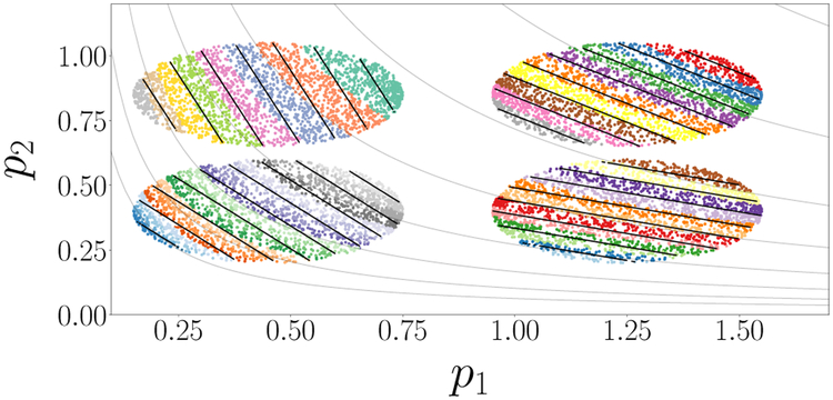
It is interesting to draw an analogy between identifying these effective parameters and the linear parameter combinations of Constantine and coworkers [3] affecting scalar model predictions: what they call “active subspaces” (see SI for a more detailed comparison). The analogy is illustrated here in Fig. 11, for which we used our first, simple model that gave rise to Fig. 1 but with the scalar output f (p) = log(p₁p₂). The active subspace approach, applied independently to each of the datasets shown as oval patches, yields the solid black direction as “neutral” and their normal as the active subspace (per patch). To enable comparison, each dataset is also colored by the value of the leading DMAPS eigenfunction ϕ₁ obtained with the output-only-informed metric. DMAPS plainly gives nonlinear “neutral” level sets (gray lines), with ϕ₁ providing a nonlinear version of an “active” parameter combination: an effective parameter. Combining the data across patches leaves our curved level sets consistent; a linear approach would encounter problems, as these level sets start curving appreciably. Two scenarios were discussed in this paper: the first, involving an output-only-informed kernel, proved useful in the data-driven study of sloppiness. Coordinates from the intrinsic model manifold geometry pulled back on the input (i.e. parameter) space provided our “effective parameters”. The second, less explored scenario involved the non-invertible case where the same model output is observed for different isolated inputs and, more generally, one has input-output relations. The simple modifications of the DMAPS metric we used to resolve this, and the connection we drew to a “measurement process history” and embedding theorems, is a simple first research step in the data-driven elucidation of complex input–output relations by designing appropriate measurement protocols. We expect that similarity measures exploiting a measurement process, rather than a single measurement (e.g. “Mahalanobis-like” pairwise similarity measures [25]) may well prove fruitful along these lines. The physical interpretability of data-discovered effective parameters can be established in a postprocessing step, by testing whether they are one-to-one, on the data, with subsets of equally many of the physical parameters.

Figure 11:

Comparison of Active Subspaces and DMAPS in local patches for a model similar to that shown in Fig. 1. See text and also SI. Here, f(p) = (log(p₁p₂)).

References

- [1].Gutenkunst RN, Waterfall JJ, Casey FP, Brown KS, Myers CR, Sethna JP, Universally sloppy parameter sensitivities in systems biology models, PLoS Comput. Biol 3 (2007) 1–8. doi: 10.1371/journal.pcbi.0030189. [DOI] [PMC free article] [PubMed] [Google Scholar]
- [2].Raue A, Kreutz C, Maiwald T, Bachmann J, Schilling M, Klingmüller U, Timmer J, Structural and practical identifiability analysis of partially observed dynamical models by exploiting the profile likelihood, BMC bioinformatics. 25 (2009) 1923–1929. [DOI] [PubMed] [Google Scholar]
- [3].Constantine PG, Dow E, Wang Q, Active subspace methods in theory and practice: applications to kriging surfaces, SIAM J. Sci. Comput 36 (2014) A1500–A1524. [Google Scholar]
- [4].Transtrum MK, Machta BB, Sethna JP, Why are nonlinear fits to data so challenging?, Phys. Rev. Lett 104 (2010) 060201. [DOI] [PubMed] [Google Scholar]
- [5].Transtrum MK, Qiu P, Model reduction by manifold boundaries, Phys. Rev. Lett 113 (2014) 098701. [DOI] [PMC free article] [PubMed] [Google Scholar]
- [6].Coifman RR, Lafon S, Diffusion maps, Appl. Comput. Harmon. Anal 21 (2006) 5–30. doi: 10.1016/j.acha.2006.04.006, special Issue: Diffusion Maps and Wavelets. [DOI] [Google Scholar]
- [7].Lafon SS, Diffusion maps and geometric harmonics, Ph.D. thesis, Yale University PhD dissertation, 2004. [Google Scholar]
- [8].Jolliffe IT, Principal component analysis and factor analysis, in: Principal component analysis, Springer, 1986, pp. 115–128. [Google Scholar]
- [9].Coifman RR, Hirn MJ, Diffusion maps for changing data, Appl. Comput. Harmon. Anal 36 (2014) 79–107. [Google Scholar]
- [10].Silver D, Hubert T, Schrittwieser J, Antonoglou I, Lai M, Guez A, Lanctot M, Sifre L, Kumaran D, Graepel T, et al. , Mastering chess and shogi by self-play with a general reinforcement learning algorithm, arXiv preprint arXiv:1712.01815 (2017). [DOI] [PubMed] [Google Scholar]
- [11].Bodenstein M, Eine theorie der photochemischen reaktionsgeschwindigkeiten, Zeitschrift für physikalische Chemie 85 (1913) 329–397. [Google Scholar]
- [12].Bello-Rivas JM, jmbr/diffusion-maps 0.0.1, 2017. doi: 10.5281/zenodo.581667. [DOI] [Google Scholar]
- [13].Rawlings JB, Ekerdt JG, Chemical reactor analysis and design fundamentals, Nob Hill Pub, Llc, 2002. [Google Scholar]
- [14].Achard P, De Schutter E, Complex parameter landscape for a complex neuron model, PLoS Comput. Biol 2 (2006) 1–11. doi: 10.1371/journal.pcbi.0020094. [DOI] [PMC free article] [PubMed] [Google Scholar]
- [15].Johnson KA, Goody RS, The original Michaelis constant: translation of the 1913 Michaelis–Menten paper, Biochemistry 50 (2011) 8264–8269. [DOI] [PMC free article] [PubMed] [Google Scholar]
- [16].Michaelis L, Menten M, Die kinetik der inwertinwirkung., Biochemestry (1913) 333–369. [Google Scholar]
- [17].Heineken F, Tsuchiya H, Aris R, On the mathematical status of the pseudo-steady state hypothesis of biochemical kinetics, Math. Biosci 1 (1967) 95–113. [Google Scholar]
- [18].Segel LA, Slemrod M, The quasi-steady-state assumption: a case study in perturbation, SIAM Rev. Soc. Ind. Appl. Math 31 (1989) 446–477. [Google Scholar]
- [19].Weisz P, Hicks J, The behaviour of porous catalyst particles in view of internal mass and heat diffusion effects, Chem. Eng. Sci 17 (1962) 265–275. doi: 10.1016/0009-2509(62)85005-2. [DOI] [Google Scholar]
- [20].Nash J, The imbedding problem for riemannian manifolds, Ann. Math (1956) 20–63. [Google Scholar]
- [21].Takens F, Detecting strange attractors in turbulence, in: Dynamical systems and turbulence, Warwick 1980, Springer, 1981, pp. 366–381. [Google Scholar]
- [22].Whitney H, The self-intersections of a smooth n-manifold in 2n-space, Ann. Math (1944) 220–246. [Google Scholar]
- [23].Chiavazzo E, Covino R, Coifman RR, Gear CW, Georgiou AS, Hummer G, Kevrekidis IG, Intrinsic map dynamics exploration for uncharted effective free-energy landscapes, Proc. Natl. Acad. Sci 114 (2017) E5494–E5503. doi: 10.1073/pnas.1621481114. [DOI] [PMC free article] [PubMed] [Google Scholar]
- [24].Georgiou AS, Bello-Rivas JM, Gear CW, Wu H-T, Chiavazzo E, Kevrekidis IG, An exploration algorithm for stochastic simulators driven by energy gradients, Entropy 19 (2017) 294. [Google Scholar]
- [25].Mahalanobis PC, On the generalized distance in statistics, Nat. Inst. of Sci. India, 1936. [Google Scholar]
Associated Data
This section collects any data citations, data availability statements, or supplementary materials included in this article.