Training Classifiers with Natural Language Explanations

Abstract

Training accurate classifiers requires many labels, but each label provides only limited information (one bit for binary classification). In this work, we propose BabbleLabble, a framework for training classifiers in which an annotator provides a natural language explanation for each labeling decision. A semantic parser converts these explanations into programmatic labeling functions that generate noisy labels for an arbitrary amount of unlabeled data, which is used to train a classifier. On three relation extraction tasks, we find that users are able to train classifiers with comparable F1 scores from 5–100× faster by providing explanations instead of just labels. Furthermore, given the inherent imperfection of labeling functions, we find that a simple rule-based semantic parser suffices.

1. Introduction

The standard protocol for obtaining a labeled dataset is to have a human annotator view each example, assess its relevance, and provide a label (e.g., positive or negative for binary classification). However, this only provides one bit of information per example. This invites the question: how can we get more information per example, given that the annotator has already spent the effort reading and understanding an example?

Previous works have relied on identifying relevant parts of the input such as labeling features (Druck et al., 2009; Raghavan et al., 2005; Liang et al., 2009), highlighting rationale phrases in text (Zaidan and Eisner, 2008; Arora and Nyberg, 2009), or marking relevant regions in images (Ahn et al., 2006). But there are certain types of information which cannot be easily reduced to annotating a portion of the input, such as the absence of a certain word, or the presence of at least two words. In this work, we tap into the power of natural language and allow annotators to provide supervision to a classifier via natural language explanations.

Specifically, we propose a framework in which annotators provide a natural language explanation for each label they assign to an example (see Figure 1). These explanations are parsed into logical forms representing labeling functions (LFs), functions that heuristically map examples to labels (Ratner et al., 2016). The labeling functions are then executed on many unlabeled examples, resulting in a large, weakly-supervised training set that is then used to train a classifier.

Figure 1:

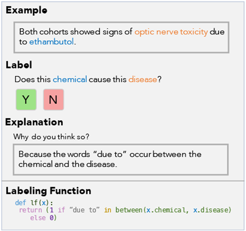
In BabbleLabble, the user provides a natural language explanation for each labeling decision. These explanations are parsed into labeling functions that convert unlabeled data into a large labeled dataset for training a classifier.

Semantic parsing of natural language into logical forms is recognized as a challenging problem and has been studied extensively (Zelle and Mooney, 1996; Zettlemoyer and Collins, 2005; Liang et al., 2011; Liang, 2016). One of our major findings is that in our setting, even a simple rule-based semantic parser suffices for three reasons: First, we find that the majority of incorrect LFs can be automatically filtered out either semantically (e.g., is it consistent with the associated example?) or pragmatically (e.g., does it avoid assigning the same label to the entire training set?). Second, LFs near the gold LF in the space of logical forms are often just as accurate (and sometimes even more accurate). Third, techniques for combining weak supervision sources are built to tolerate some noise (Alfonseca et al., 2012; Takamatsu et al., 2012; Ratner et al., 2018). The significance of this is that we can deploy the same semantic parser across tasks without task-specific training. We show how we can tackle a real-world biomedical application with the same semantic parser used to extract instances of spouses.

Our work is most similar to that of Srivastava et al. (2017), who also use natural language explanations to train a classifier, but with two important differences. First, they jointly train a task-specific semantic parser and classifier, whereas we use a simple rule-based parser. In Section 4, we find that in our weak supervision framework, the rule-based semantic parser and the perfect parser yield nearly identical downstream performance. Second, while they use the logical forms of explanations to produce features that are fed directly to a classifier, we use them as functions for labeling a much larger training set. In Section 4, we show that using functions yields a 9.5 F1 improvement (26% relative improvement) over features, and that the F1 score scales with the amount of available unlabeled data.

We validate our approach on two existing datasets from the literature (extracting spouses from news articles and disease-causing chemicals from biomedical abstracts) and one real-world use case with our biomedical collaborators at OccamzRazor to extract protein-kinase interactions related to Parkinson’s disease from text. We find empirically that users are able to train classifiers with comparable F1 scores up to 100× faster when they provide natural language explanations instead of individual labels. Our code is available at https://github.com/HazyResearch/babble.

2. The BabbleLabble Framework

The BabbleLabble framework converts natural language explanations and unlabeled data into a noisily-labeled training set (see Figure 2). There are three key components: a semantic parser, a filter bank, and a label aggregator. The semantic parser converts natural language explanations into a set of logical forms representing labeling functions (LFs). The filter bank removes as many incorrect LFs as possible without requiring ground truth labels. The remaining LFs are applied to unlabeled examples to produce a matrix of labels. This label matrix is passed into the label aggregator, which combines these potentially conflicting and overlapping labels into one label for each example. The resulting labeled examples are then used to train an arbitrary discriminative model.

Figure 2:

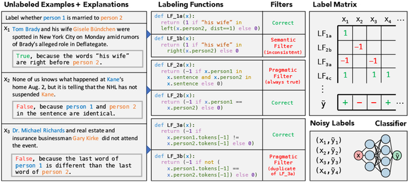
Natural language explanations are parsed into candidate labeling functions (LFs). Many incorrect LFs are filtered out automatically by the filter bank. The remaining functions provide heuristic labels over the unlabeled dataset, which are aggregated into one noisy label per example, yielding a large, noisily-labeled training set for a classifier.

2.1. Explanations

To create the input explanations, the user views a subset S of an unlabeled dataset D (where |S| ≪ |D|) and provides for each input x_i ∈ S a label y_i and a natural language explanation e_i a sentence explaining why the example should receive that label. The explanation e_i generally refers to specific aspects of the example (e.g., in Figure 2, the location of a specific string “his wife”).

2.2. Semantic Parser

The semantic parser takes a natural language explanation e_i and returns a set of LFs (logical forms or labeling functions) {f₁, … , f_k} of the form f_i : χ → {−1, 0, 1} in a binary classification setting, with 0 representing abstention. We emphasize that the goal of this semantic parser is not to generate the single correct parse, but rather to have coverage over many potentially useful LFs.¹

We choose a simple rule-based semantic parser that can be used without any training. Formally, the parser uses a set of rules of the form α → β, where α can be replaced by the token(s) in β (see Figure 3 for example rules). To identify candidate LFs, we recursively construct a set of valid parses for each span of the explanation, based on the substitutions defined by the grammar rules. At the end, the parser returns all valid parses (LFs in our case) corresponding to the entire explanation.

Figure 3:

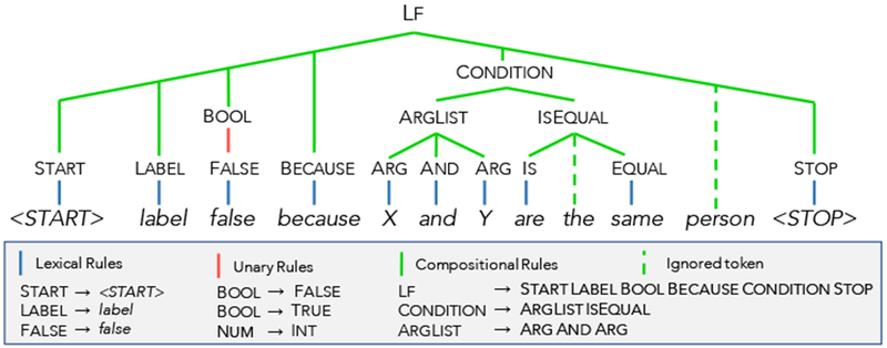
Valid parses are found by iterating over increasingly large subspans of the input looking for matches among the right hand sides of the rules in the grammar. Rules are either lexical (converting tokens into symbols), unary (converting one symbol into another symbol), or compositional (combining many symbols into a single higher-order symbol). A rule may optionally ignore unrecognized tokens in a span (denoted here with a dashed line).

We also allow an arbitrary number of tokens in a given span to be ignored when looking for a matching rule. This improves the ability of the parser to handle unexpected input, such as unknown words or typos, since the portions of the input that are parseable can still result in a valid parse. For example, in Figure 3, the word “person” is ignored.

All predicates included in our grammar (summarized in Table 1) are provided to annotators, with minimal examples of each in use (Appendix A). Importantly, all rules are domain independent (e.g., all three relation extraction tasks that we tested used the same grammar), making the semantic parser easily transferrable to new domains. Additionally, while this paper focuses on the task of relation extraction, in principle the BabbleLabble framework can be applied to other tasks or settings by extending the grammar with the necessary primitives (e.g., adding primitives for rows and columns to enable explanations about the alignments of words in tables). To guide the construction of the grammar, we collected 500 explanations for the Spouse domain from workers on Amazon Mechanical Turk and added support for the most commonly used predicates. These were added before the experiments described in Section 4. The grammar contains a total of 200 rule templates.

Table 1:

Predicates in the grammar supported by BabbleLabble’s rule-based semantic parser.

Predicate	Description
bool, string, int, float, tuple, list, set	Standard primitive data types
and, or, not, any, all, none	Standard logic operators
=, ≠, <, ≤, >, ≥	Standard comparison operators
lower, upper, capital, all_caps	Return True for strings of the corresponding case
starts_with, ends_with, substring	Return True if the first string starts/ends with or contains the second
person, location, date, number, organization alias	Return True if a string has the corresponding NER tag
	A frequently used list of words may be predefined and referred to with an alias
count, contains, intersection	Operators for checking size, membership, or common elements of a list/set
map, filter	Apply a functional primitive to each member of list/set to transform or filter the elements
word_distance, character_distance	Return the distance between two strings by words or characters
left, right, between, within	Return as a string the text that is left/right/within some distance of a string or between two designated strings

2.3. Filter Bank

The input to the filter bank is a set of candidate LFs produced by the semantic parser. The purpose of the filter bank is to discard as many incorrect LFs as possible without requiring additional labels. It consists of two classes of filters: semantic and pragmatic.

Recall that each explanation e_i is collected in the context of a specific labeled example (x_i, y_i). The semantic filter checks for LFs that are inconsistent with their corresponding example; formally, any LF f for which f(x_i) ≠ y_i is discarded. For example, in the first explanation in Figure 2, the word “right” can be interpreted as either “immediately” (as in “right before”) or simply “to the right.” The latter interpretation results in a function that is inconsistent with the associated example (since “his wife” is actually to the left of person 2), so it can be safely removed.

The pragmatic filters removes LFs that are constant, redundant, or correlated. For example, in Figure 2, LF_2a is constant, as it labels every example positively (since all examples contain two people from the same sentence). LF_3b is redundant, since even though it has a different syntax tree from LF_3a, it labels the training set identically and therefore provides no new signal.

Finally, out of all LFs from the same explanation that pass all the other filters, we keep only the most specific (lowest coverage) LF. This prevents multiple correlated LFs from a single example from dominating.

As we show in Section 4, over three tasks, the filter bank removes over 95% of incorrect parses, and the incorrect ones that remain have average end-task accuracy within 2.5 points of the corresponding correct parses.

2.4. Label Aggregator

The label aggregator combines multiple (potentially conflicting) suggested labels from the LFs and combines them into a single probabilistic label per example. Concretely, if m LFs pass the filter bank and are applied to n examples, the label aggregator implements a function f : {−1, 0, 1}^m×n → [0, 1]ⁿ.

A naive solution would be to use a simple majority vote, but this fails to account for the fact that LFs can vary widely in accuracy and coverage. Instead, we use data programming (Ratner et al., 2016), which models the relationship between the true labels and the output of the labeing functions as a factor graph. More specifically, given the true labels Y ∈ {−1, 1}ⁿ (latent) and label matrix Λ ∈ {−1, 0, 1}^m×n (observed) where Λ_i,j = LF_i(x_j), we define two types of factors representing labeling propensity and accuracy:

$${\varphi }_{i,j}^{\text{Lab}}(\Lambda ,Y)=\mathbb{1}\left\{{\Lambda }_{i,j}\ne 0\right\}$$ (1)

$${\varphi }_{i,j}^{\text{Acc}}(\Lambda ,Y)=\mathbb{1}\left\{{\Lambda }_{i,j}=yj\right\}.$$ (2)

Denoting the vector of factors pertaining to a given data point x_j as ϕ_j (Λ, Y) ∈ ${\mathbb{R}}^m$, define the model:

$$p_{{}_w}(\Lambda ,Y)=Z_w^{-1}\text{exp}\left(\sum _{j=i}^{n}w\cdot {\varphi }_j(\Lambda ,Y)\right),$$ (3)

where w ∈ ${\mathbb{R}}^{2m}$ is the weight vector and Z_w is the normalization constant. To learn this model without knowing the true labels Y, we minimize the negative log marginal likelihood given the observed labels Λ:

$$\widehat{w}={\text{arg}}_w\text{min}-\text{log}\sum _Y{p}_w(\Lambda ,Y)$$ (4)

using SGD and Gibbs sampling for inference, and then use the marginals $p_{\widehat{w}}$(Y | Λ) as probabilistic training labels.

Intuitively, we infer accuracies of the LFs based on the way they overlap and conflict with one another. Since noisier LFs are more likely to have high conflict rates with others, their corresponding accuracy weights in w will be smaller, reducing their influence on the aggregated labels.

2.5. Discriminative Model

The noisy training set that the label aggregator outputs is used to train an arbitrary discriminative model. One advantage of training a discriminative model on the task instead of using the label aggregator as a classifier directly is that the label aggregator only takes into account those signals included in the LFs. A discriminative model, on the other hand, can incorporate features that were not identified by the user but are nevertheless informative.² Consequently, even examples for which all LFs abstained can still be classified correctly. Additionally, passing supervision information from the user to the model in the form of a dataset—rather than hard rules—promotes generalization in the new model (rather than memorization), similar to distant supervision (Mintz et al., 2009). On the three tasks we evaluate, using the discriminative model averages 4.3 F1 points higher than using the label aggregator directly.

For the results reported in this paper, our discriminative model is a simple logistic regression classifier with generic features defined over dependency paths.³ These features include unigrams, bigrams, and trigrams of lemmas, dependency labels, and part of speech tags found in the siblings, parents, and nodes between the entities in the dependency parse of the sentence. We found this to perform better on average than a biLSTM, particularly for the traditional supervision baselines with small training set sizes; it also provided easily interpretable features for analysis.

3. Experimental Setup

We evaluate the accuracy of BabbleLabble on three relation extraction tasks, which we refer to as Spouse, Disease, and Protein. The goal of each task is to train a classifier for predicting whether the two entities in an example are participating in the relationship of interest, as described below.

3.1. Datasets

Statistics for each dataset are reported in Table 2, with one example and one explanation for each given in Figure 4 and additional explanations shown in Appendix B.

Table 2:

The total number of unlabeled training examples (a pair of annotated entities in a sentence), labeled development examples (for hyperparameter tuning), labeled test examples (for assessment), and the fraction of positive labels in the test split.

Task	Train	Dev	Test	% Pos.
Spouse	22195	2796	2697	8%
Disease	6667	773	4101	23%
Protein	5546	1011	1058	22%

Figure 4:

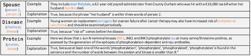
An example and explanation for each of the three datasets.

In the Spouse task, annotators were shown a sentence with two highlighted names and asked to label whether the sentence suggests that the two people are spouses. Sentences were pulled from the Signal Media dataset of news articles (Corney et al., 2016). Ground truth data was collected from Amazon Mechanical Turk workers, accepting the majority label over three annotations. The 30 explanations we report on were sampled randomly from a pool of 200 that were generated by 10 graduate students unfamiliar with BabbleLabble.

In the Disease task, annotators were shown a sentence with highlighted names of a chemical and a disease and asked to label whether the sentence suggests that the chemical causes the disease. Sentences and ground truth labels came from a portion of the 2015 BioCreative chemical-disease relation dataset (Wei et al., 2015), which contains abstracts from PubMed. Because this task requires specialized domain expertise, we obtained explanations by having someone unfamiliar with BabbleLabble translate from Python to natural language labeling functions from an existing publication that explored applying weak supervision to this task (Ratner et al., 2018).

The Protein task was completed in conjunction with OccamzRazor, a neuroscience company targeting biological pathways of Parkinson’s disease. For this task, annotators were shown a sentence from the relevant biomedical literature with highlighted names of a protein and a kinase and asked to label whether or not the kinase influences the protein in terms of a physical interaction or phosphorylation. The annotators had domain expertise but minimal programming experience, making BabbleLabble a natural fit for their use case.

3.2. Experimental Settings

Text documents are tokenized with spaCy.⁴ The semantic parser is built on top of the Python-based implementation SippyCup.⁵ On a single core, parsing 360 explanations takes approximately two seconds. We use existing implementations of the label aggregator, feature library, and discriminative classifier described in Sections 2.4—2.5 provided by the open-source project Snorkel (Ratner et al., 2018).

Hyperparameters for all methods we report were selected via random search over thirty configurations on the same held-out development set. We searched over learning rate, batch size, L₂ regularization, and the subsampling rate (for improving balance between classes).⁶ All reported F1 scores are the average value of 40 runs with random seeds and otherwise identical settings.

4. Experimental Results

We evaluate the performance of BabbleLabble with respect to its rate of improvement by number of user inputs, its dependence on correctly parsed logical forms, and the mechanism by which it utilizes logical forms.

4.1. High Bandwidth Supervision

In Table 3 we report the average F1 score of a classifier trained with BabbleLabble using 30 explanations or traditional supervision with the indicated number of labels. On average, it took the same amount of time to collect 30 explanations as 60 labels.⁷ We observe that in all three tasks, BabbleLabble achieves a given F1 score with far fewer user inputs than traditional supervision, by as much as 100 times in the case of the Spouse task. Because explanations are applied to many unlabeled examples, each individual input from the user can implicitly contribute many (noisy) labels to the learning algorithm.

Table 3:

F1 scores obtained by a classifier trained with BabbleLabble (BL) using 30 explanations or with traditional supervision (TS) using the specified number of individually labeled examples. BabbleLabble achieves the same F1 score as traditional supervision while using fewer user inputs by a factor of over 5 (Protein) to over 100 (Spouse).

# Inputs	BL	TS
	30	30	60	150	300	1,000	3,000	10,000
Spouse	50.1	15.5	15.9	16.4	17.2	22.8	41.8	55.0
Disease	42.3	32.1	32.6	34.4	37.5	41.9	44.5	-
Protein	47.3	39.3	42.1	46.8	51.0	57.6	-	-
Average	46.6	28.9	30.2	32.5	35.2	40.8	43.2	55.0

We also observe, however, that once the number of labeled examples is sufficiently large, traditional supervision once again dominates, since ground truth labels are preferable to noisy ones generated by labeling functions. However, in domains where there is much more unlabeled data available than labeled data (which in our experience is most domains), we can gain in supervision efficiency from using BabbleLabble.

Of those explanations that did not produce a correct LF, 4% were caused by the explanation referring to unsupported concepts (e.g., one explanation referred to “the subject of the sentence,” which our simple parser doesn’t support). Another 2% were caused by human errors (the correct LF for the explanation was inconsistent with the example). The remainder were due to unrecognized paraphrases (e.g., the explanation said “the order of appearance is X, Y” instead of a supported phrasing like “X comes before Y”).

4.2. Utility of Incorrect Parses

In Table 4, we report LF summary statistics before and after filtering. LF correctness is based on exact match with a manually generated parse for each explanation. Surprisingly, the simple heuristic-based filter bank successfully removes over 95% of incorrect LFs in all three tasks, resulting in final LF sets that are 86% correct on average. Furthermore, among those LFs that pass through the filter bank, we found that the average difference in end-task accuracy between correct and incorrect parses is less than 2.5%. Intuitively, the filters are effective because it is quite difficult for an LF to be parsed from the explanation, label its own example correctly (passing the semantic filter), and not label all examples in the training set with the same label or identically to another LF (passing the pragmatic filter).

Table 4:

The number of LFs generated from 30 explanations (pre-filters), discarded by the filter bank, and remaining (post-filters), along with the percentage of LFs that were correctly parsed from their corresponding explanations.

	Pre-filters		Discarded		Post-filters
	LFs	Correct	Sem.	Prag.	LFs	Correct
Spouse	156	10%	19	118	19	84%
Disease	102	23%	34	40	28	89%
Protein	122	14%	44	58	20	85%

We went one step further: using the LFs that would be produced by a perfect semantic parser as starting points, we searched for “nearby” LFs (LFs differing by only one predicate) with higher end-task accuracy on the test set and succeeded 57% of the time (see Figure 5 for an example). In other words, when users provide explanations, the signals they describe provide good starting points, but they are actually unlikely to be optimal. This observation is further supported by Table 5, which shows that the filter bank is necessary to remove clearly irrelevant LFs, but with that in place, the simple rule-based semantic parser and a perfect parser have nearly identical average F1 scores.

Figure 5:

Incorrect LFs often still provide useful signal. On top is an incorrect LF produced for the Disease task that had the same accuracy as the correct LF. On bottom is a correct LF from the Spouse task and a more accurate incorrect LF discovered by randomly perturbing one predicate at a time as described in Section 4.2. (Person 2 is always the second person in the sentence).

Table 5:

F1 scores obtained using BabbleLabble with no filter bank (BL-FB), as normal (BL), and with a perfect parser (BL+PP) simulated by hand.

	BL-FB	BL	BL+PP
Spouse	15.7	50.1	49.8
Disease	39.8	42.3	43.2
Protein	38.2	47.3	47.4
Average	31.2	46.6	46.8

4.3. Using LFs as Functions or Features

Once we have relevant logical forms from user-provided explanations, we have multiple options for how to use them. Srivastava et al. (2017) propose using these logical forms as features in a linear classifier, essentially using a traditional supervision approach with user-specified features. We choose instead to use them as functions for weakly supervising the creation of a larger training set via data programming (Ratner et al., 2016). In Table 6, we compare the two approaches directly, finding that the the data programming approach outperforms a feature-based one by 9.5 F1 points on average with the rule-based parser, and by 4.5 points with a perfect parser.

Table 6:

F1 scores obtained using explanations as functions for data programming (BL) or features (Feat), optionally with no discriminative model (−DM) or using a perfect parser (+PP).

	BL-DM	BL	BL+PP	Feat	Feat+PP
Spouse	46.5	50.1	49.8	33.9	39.2
Disease	39.7	42.3	43.2	40.8	43.8
Protein	40.6	47.3	47.4	36.7	44.0
Average	42.3	46.6	46.8	37.1	42.3

We attribute this difference primarily to the ability of data programming to utilize a larger feature set and unlabeled data. In Figure 6, we show how the data programming approach improves with the number of unlabeled examples, even as the number of LFs remains constant. We also observe qualitatively that data programming exposes the classifier to additional patterns that are correlated with our explanations but not mentioned directly. For example, in the Disease task, two of the features weighted most highly by the discriminative model were the presence of the trigrams “could produce a” or “support diagnosis of” between the chemical and disease, despite none of these words occurring in the explanations for that task. In Table 6 we see a 4.3 F1 point improvement (10%) when we use the discriminative model that can take advantage of these features rather than applying the LFs directly to the test set and making predictions based on the label aggregator’s outputs.

Figure 6:

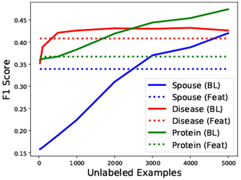
When logical forms of natural language explanations are used as functions for data programming (as they are in BabbleLabble), performance can improve with the addition of unlabeled data, whereas using them as features does not benefit from unlabeled data.

5. Related Work and Discussion

Our work has two themes: modeling natural language explanations/instructions and learning from weak supervision. The closest body of work is on “learning from natural language.” As mentioned earlier, Srivastava et al. (2017) convert natural language explanations into classifier features (whereas we convert them into labeling functions). Goldwasser and Roth (2011) convert natural language into concepts (e.g., the rules of a card game). Ling and Fidler (2017) use natural language explanations to assist in supervising an image captioning model. Weston (2016); Li et al. (2016) learn from natural language feedback in a dialogue. Wang et al. (2017) convert natural language definitions to rules in a semantic parser to build up progressively higher-level concepts.

We lean on the formalism of semantic parsing (Zelle and Mooney, 1996; Zettlemoyer and Collins, 2005; Liang, 2016). One notable trend is to learn semantic parsers from weak supervision (Clarke et al., 2010; Liang et al., 2011), whereas our goal is to obtain weak supervision signal from semantic parsers.

The broader topic of weak supervision has received much attention; we mention some works most related to relation extraction. In distant supervision (Craven et al., 1999; Mintz et al., 2009) and multi-instance learning (Riedel et al., 2010; Hoffmann et al., 2011), an existing knowledge base is used to (probabilistically) impute a training set. Various extensions have focused on aggregating a variety of supervision sources by learning generative models from noisy labels (Alfonseca et al., 2012; Takamatsu et al., 2012; Roth and Klakow, 2013; Ratner et al., 2016; Varma et al., 2017).

Finally, while we have used natural language explanations as input to train models, they can also be output to interpret models (Krening et al., 2017; Lei et al., 2016). More generally, from a machine learning perspective, labels are the primary asset, but they are a low bandwidth signal between annotators and the learning algorithm. Natural language opens up a much higher-bandwidth communication channel. We have shown promising results in relation extraction (where one explanation can be “worth” 100 labels), and it would be interesting to extend our framework to other tasks and more interactive settings.

A Predicate Examples

Below are the predicates in the rule-based semantic parser grammar, each of which may have many supported paraphrases, only one of which is listed here in a minimal example.

Logic

and: X is true and Y is true

or: X is true or Y is true

not: X is not true

any: Any of X or Y or Z is true

all: All of X and Y and Z are true

none: None of X or Y or Z is true

Comparison

=: X is equal to Y

≠: X is not Y

<: X is smaller than Y

≤: X is no more than Y

>: X is larger than Y

≥: X is at least Y

Syntax

lower: X is lowercase

upper: X is upper case

capital: X is capitalized

all_caps: X is in all caps

starts_with: X starts with “cardio”

ends_with: X ends with “itis”

substring: X contains “–induced”

Named-entity Tags

person: A person is between X and Y

location: A place is within two words of X

date: A date is between X and Y

number: There are three numbers in the sentence

organization: An organization is right after X

Lists

list: (X, Y) is in Z

set: X, Y, and Z are true

count: There is one word between X and Y

contains: X is in Y

intersection: At least two of X are in Y

map: X is at the start of a word in Y

filter: There are three capitalized words to the left of X

alias: A spouse word is in the sentence (“spouse” is a predefined list from the user)

Position

word_distance: X is two words before Y

char_distance: X is twenty characters after Y

left: X is before Y

right: X is after Y

between: X is between Y and Z

within: X is within five words of Y

B Sample Explanations

The following are a sample of the explanations provided by users for each task.

Spouse

Users referred to the first person in the sentence as “X” and the second as “Y”.

Label true because “and” occurs between X and Y and “marriage” occurs one word after person1.

Label true because person Y is preceded by ‘beau’.

Label false because the words “married”, “spouse”, “husband”, and “wife” do not occur in the sentence.

Label false because there are more than 2 people in the sentence and “actor” or “actress” is left of person1 or person2.

Disease

Label true because the disease is immediately after the chemical and ‘induc’ or ‘assoc’ is in the chemical name.

Label true because a word containing ‘develop’ appears somewhere before the chemical, and the word ‘following’ is between the disease and the chemical.

Label true because “induced by”, “caused by”, or “due to” appears between the chemical and the disease.”

Label false because “none”, “not”, or “no” is within 30 characters to the left of the disease.

Protein

Label true because “Ser” or “Tyr” are within 10 characters of the protein.

Label true because the words “by” or “with” are between the protein and kinase and the words “no”, “not” or “none” are not in between the protein and kinase and the total number of words between them is smaller than 10.

Label false because the sentence contains “mRNA”, “DNA”, or “RNA”.

Label false because there are two “,” between the protein and the kinase with less than 30 characters between them.

References

- Ahn LV, Liu R, and Blum M. 2006. Peekaboom: a game for locating objects in images. In Conference on Human Factors in Computing Systems (CHI). pages 55–64. [Google Scholar]
- Alfonseca E, Filippova K, Delort J, and Garrido G. 2012. Pattern learning for relation extraction with a hierarchical topic model. In Association for Computational Linguistics (ACL). pages 54–59. [Google Scholar]
- Arora S and Nyberg E. 2009. Interactive annotation learning with indirect feature voting. In Association for Computational Linguistics (ACL). pages 55–60. [Google Scholar]
- Clarke J, Goldwasser D, Chang M, and Roth D. 2010. Driving semantic parsing from the world’s response. In Computational Natural Language Learning (CoNLL). pages 18–27. [Google Scholar]
- Corney D, Albakour D, Martinez-Alvarez M, and Moussa S. 2016. What do a million news articles look like? In NewsIR@ ECIR. pages 42–47. [Google Scholar]
- Craven M, Kumlien J, et al. 1999. Constructing biological knowledge bases by extracting information from text sources. In ISMB. pages 77–86. [PubMed] [Google Scholar]
- Druck G, Settles B, and McCallum A. 2009. Active learning by labeling features. In Empirical Methods in Natural Language Processing (EMNLP). pages 81–90. [Google Scholar]
- Goldwasser D and Roth D. 2011. Learning from natural instructions. In International Joint Conference on Artificial Intelligence (IJCAI). pages 1794–1800. [Google Scholar]
- Hoffmann R, Zhang C, Ling X, Zettlemoyer LS, and Weld DS. 2011. Knowledge-based weak supervision for information extraction of overlapping relations. In Association for Computational Linguistics (ACL). pages 541–550. [Google Scholar]
- Krening S, Harrison B, Feigh KM, Isbell CL, Riedl M, and Thomaz A. 2017. Learning from explanations using sentiment and advice in RL. IEEE Transactions on Cognitive and Developmental Systems 9(1):44–55. [Google Scholar]
- Lei T, Barzilay R, and Jaakkola T. 2016. Rationalizing neural predictions. In Empirical Methods in Natural Language Processing (EMNLP). [Google Scholar]
- Li J, Miller AH, Chopra S, Ranzato M, and Weston J. 2016. Learning through dialogue interactions. arXiv preprint arXiv:1612.04936. [Google Scholar]
- Liang P. 2016. Learning executable semantic parsers for natural language understanding. Communications of the ACM 59. [Google Scholar]
- Liang P, Jordan MI, and Klein D. 2009. Learning from measurements in exponential families. In International Conference on Machine Learning (ICML). [Google Scholar]
- Liang P, Jordan MI, and Klein D. 2011. Learning dependency-based compositional semantics. In Association for Computational Linguistics (ACL). pages 590–599. [Google Scholar]
- Ling H and Fidler S. 2017. Teaching machines to describe images via natural language feedback. In Advances in Neural Information Processing Systems (NIPS). [Google Scholar]
- Mintz M, Bills S, Snow R, and Jurafsky D. 2009. Distant supervision for relation extraction without labeled data. In Association for Computational Linguistics (ACL). pages 1003–1011. [Google Scholar]
- Raghavan H, Madani O, and Jones R. 2005. Interactive feature selection. In International Joint Conference on Artificial Intelligence (IJCAI). volume 5, pages 841–846. [Google Scholar]
- Ratner AJ, Bach SH, Ehrenberg H, Fries J, Wu S, and R’e C. 2018. Snorkel: Rapid training data creation with weak supervision. In Very Large Data Bases (VLDB). [DOI] [PMC free article] [PubMed] [Google Scholar]
- Ratner AJ, Sa CMD, Wu S, Selsam D, and R’e C. 2016. Data programming: Creating large training sets, quickly. In Advances in Neural Information Processing Systems (NIPS). pages 3567–3575. [PMC free article] [PubMed] [Google Scholar]
- Riedel S, Yao L, and McCallum A. 2010. Modeling relations and their mentions without labeled text. In Machine Learning and Knowledge Discovery in Databases (ECML PKDD). pages 148–163. [Google Scholar]
- Roth B and Klakow D. 2013. Combining generative and discriminative model scores for distant supervision. In Empirical Methods in Natural Language Processing (EMNLP). pages 24–29. [Google Scholar]
- Srivastava S, Labutov I, and Mitchell T. 2017. Joint concept learning and semantic parsing from natural language explanations. In Empirical Methods in Natural Language Processing (EMNLP). pages 1528–1537. [Google Scholar]
- Takamatsu S, Sato I, and Nakagawa H. 2012. Reducing wrong labels in distant supervision for relation extraction. In Association for Computational Linguistics (ACL). pages 721–729. [Google Scholar]
- Varma P, He B, Iter D, Xu P, Yu R, Sa CD, and R’e C. 2017. Socratic learning: Augmenting generative models to incorporate latent subsets in training data. arXiv preprint arXiv:1610.08123 . [Google Scholar]
- Wang SI, Ginn S, Liang P, and Manning CD. 2017. Naturalizing a programming language via interactive learning. In Association for Computational Linguistics (ACL). [Google Scholar]
- Wei C, Peng Y, Leaman R, Davis AP, Mattingly CJ, Li J, Wiegers TC, and Lu Z. 2015. Overview of the biocreative V chemical disease rlation (cdr) task. In Proceedings of the fifth BioCreative challenge evaluation workshop. pages 154–166. [Google Scholar]
- Weston JE. 2016. Dialog-based language learning. In Advances in Neural Information Processing Systems (NIPS). pages 829–837. [Google Scholar]
- Zaidan OF and Eisner J. 2008. Modeling annotators: A generative approach to learning from annotator rationales. In Empirical Methods in Natural Language Processing (EMNLP). [Google Scholar]
- Zelle M and Mooney RJ. 1996. Learning to parse database queries using inductive logic programming. In Association for the Advancement of Artificial Intelligence (AAAI). pages 1050–1055. [Google Scholar]
- Zettlemoyer LS and Collins M. 2005. Learning to map sentences to logical form: Structured classification with probabilistic categorial grammars. In Uncertainty in Artificial Intelligence (UAI). pages 658–666. [Google Scholar]