Experimental investigation of performance differences between coherent Ising machines and a quantum annealer

Benchmarking the coherent Ising machine and the D-Wave quantum annealer sheds light on the importance of connectivity.

Abstract

Physical annealing systems provide heuristic approaches to solving combinatorial optimization problems. Here, we benchmark two types of annealing machines—a quantum annealer built by D-Wave Systems and measurement-feedback coherent Ising machines (CIMs) based on optical parametric oscillators—on two problem classes, the Sherrington-Kirkpatrick (SK) model and MAX-CUT. The D-Wave quantum annealer outperforms the CIMs on MAX-CUT on cubic graphs. On denser problems, however, we observe an exponential penalty for the quantum annealer [exp(–α_DWN²)] relative to CIMs [exp(–α_CIMN)] for fixed anneal times, both on the SK model and on 50% edge density MAX-CUT. This leads to a several orders of magnitude time-to-solution difference for instances with over 50 vertices. An optimal–annealing time analysis is also consistent with a substantial projected performance difference. The difference in performance between the sparsely connected D-Wave machine and the fully-connected CIMs provides strong experimental support for efforts to increase the connectivity of quantum annealers.

INTRODUCTION

Optimization problems are ubiquitous in science, engineering, and business. Many important problems (especially combinatorial problems such as scheduling, resource allocation, route planning, or community detection) belong to the nondeterministic polynomial time (NP)–hard complexity class and, even for typical instances, require a computation time that scales exponentially with the problem size (1). Canonical examples such as Karp’s 21 NP-complete problems (2) have attracted much attention from researchers seeking to devise new optimization methods because, by definition, any NP-complete problem can be reduced to any other problem in NP with only polynomial overhead. Many approximation algorithms and heuristics [e.g., relaxations to semidefinite programs (3), simulated annealing (4), and breakout local search (BLS) (5)] have been developed to search for good-quality approximate solutions and ground states for sufficiently small problem sizes. However, for many NP-hard optimization problems, even moderately sized problem instances can be time consuming to solve exactly or even approximately. Hence, there is a strong motivation to find alternative approaches that can consistently beat state-of-the-art algorithms.

Despite decades of Moore’s law scaling, large NP-hard problems remain very costly even on modern microprocessors. Thus, there is a growing interest in special-purpose machines that implement a solver directly by mapping the optimization to the underlying physical dynamics. Examples include digital complementary metal-oxide semiconductor annealers (6, 7) and analog devices such as nanomagnet arrays (8), electronic oscillators (9, 10), and laser networks (11). Quantum adiabatic computation (12) and quantum annealing (13–16) are also prominent examples and may offer the possibility of quantum speedup (17–19) for certain NP-hard problems. However, all the nonphotonic analog optimization systems realized to date suffer from limited connectivity so that actual problems must, in general, first be embedded (20, 21) into the solver architecture native graph before they can be solved. This requirement adds an upfront computational cost (20, 22, 23) of finding the embedding (unless previously known) and, of most relevance in this study, in general results in the use of multiple physical pseudo-spins to encode each logical spin variable, which can lead to a degradation of time to solution.

Here, we perform the first direct comparison between the D-Wave 2000Q (DW2Q) quantum annealer and the coherent Ising machine (CIM) (24, 25). As we will see later, a crucial distinction between these systems is their intrinsic connectivity, which has a profound influence on their performance. Both systems are designed to solve the classical Ising problem, that is, to minimize the classical Hamiltonian

$$H=\frac{1}{2}{\displaystyle \sum _{\mathit{ij}}}{J}_{\mathit{ij}}{\mathrm{\sigma }}_i{\mathrm{\sigma }}_j+{\displaystyle \sum _i}{h}_i{\mathrm{\sigma }}_i$$ (1)

where σ_i = ±1 are the Ising spins, J_ij are the entries of the spin-spin coupling matrix, and h_i are the Zeeman (bias) terms. The Ising problem is NP-hard for nonplanar couplings (26) and is one of the most widely studied problems in this complexity class. We focus on two canonical NP-hard Ising problems: unweighted MAX-CUT (2) and ground-state computation of the Sherrington-Kirkpatrick (SK) spin-glass model (27).

In the CIM, the spin network is represented by a network of degenerate optical parametric oscillators (OPOs). Each OPO is a nonlinear oscillator that converts pump light to its half-harmonic (28); it can oscillate in two identical phase states, which encode the value of the Ising spin (29, 30). Optical coherence is essential to the CIM, where the data are encoded in the phase of the light. As Fig. 1A shows, time multiplexing offers a straightforward way to generate many identical OPOs in a single cavity (30). A pulsed laser with repetition time T is used to pump an optical cavity with round-trip time N × T. Parametric amplification is provided by the χ⁽²⁾ crystal; since this is an instantaneous nonlinearity, the circulating pulses in the cavity are identical and noninteracting. The approach is scalable using high–repetition rate lasers and long fiber cavities: OPO gain has been reported for up to N = 10⁶ pulses, and stable operation achieved for N = 50,000 (31). Each circulating pulse represents an independent OPO with a single degree of freedom, a_i. Classically, a_i is a complex variable, which maps to the annihilation operator ${\widehat{a}}_i$ in quantum mechanics (32). A measurement-feedback apparatus is used to apply coupling between the pulses (24, 25). In each round trip, a small fraction of the light (~10%) is extracted from the cavity and homodyned against a reference pulse (the OPO pump is created from second harmonic generation of the reference laser, so there is good matching between the reference and the OPO signal light, which is at half the frequency of the pump). The homodyne result, in essence a measurement of a_i, is fed into an electronic circuit (consisting of an analog-to-digital converter, a field-programmable gate array, and a digital-to-analog converter) that, for each pulse, computes a feedback signal that is proportional to the matrix-vector product ∑_jJ_ija_j. This signal is converted back to light using an optical modulator and a reference pulse and reinjected into the cavity. The measurement-feedback CIM has intrinsic all-to-all connectivity through its exploitation of memory in the electronic circuit [although the same effect can be obtained with optical delay-line memories in all-optical CIMs (29, 30)].

Fig. 1. Schematic and operation principle of the CIM.

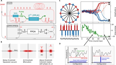
(A) CIM design consisting of time-multiplexed OPO and measurement-feedback apparatus. See (24, 25) for details. SHG, second harmonic generation; FPGA, field-programmable gate array; PPLN, periodically poled lithium niobate; IM, intensity modulator; PM, phase modulator. (B) OPO state during transition from below-threshold squeezed state to (bistable) above-threshold coherent state. (C) Solution of antiferromagnetic Ising problem on the Möbius ladder with the CIM, giving measured OPO amplitudes a_i and Ising energy H as a function of time in round trips. (D) Illustration of search-from-below principle of CIM operation.

The OPO is a dissipative quantum system with a pitchfork bifurcation well adapted for modeling Ising spins: As the pump power is increased (Fig. 1B), the OPO state transitions from a below-threshold squeezed vacuum state (33–35) to an above-threshold coherent state (36). Because degenerate parametric amplification is phase sensitive, only two phase states are stable above threshold; thus, the OPO functions as a classical “spin” with states {∣0〉, ∣π〉} that can be mapped to the Ising states σ_i = { + 1, − 1}. The optimization process happens in the near-threshold regime where the dynamics are determined by a competition between the network loss and Ising coupling (which seek to minimize the product ∑_ijJ_ija_ia_j), as well as nonlinear parametric gain (which seeks to enforce the constraints a_i ∈ ℝ, ∣a_i∣ = const).

As an example, consider the Ising problem on the N = 16 Möbius ladder graph with antiferromagnetic couplings (37). Figure 1C shows a typical run of the CIM, resulting in a solution that minimizes the Ising energy [data from (24)]. The most obvious interpretation of the process is spontaneous symmetry breaking of a pitchfork bifurcation: Prepared in a squeezed vacuum state and driven by shot noise, the OPO state bifurcates, during which its amplitudes a_i grow either in positive or negative value, and subsequently the system settles into the Ising ground state (or a low-lying excited state) (24, 38) [this is related to the Gaussian state model in (39)]. Another view derives from ground-state “search from below” (Fig. 1D). Here, the Ising energy is visualized as a complicated landscape of potential oscillation thresholds, each with its own spin configuration. If the OPO pump is far below the minimum threshold, all spin configurations will be excited with near-equal probability, but once the ground-state threshold is exceeded, its probability will grow exponentially at the expense of other configurations (30, 40). This ground-state selection process corresponds to the 40 ≤ t ≤ 60 region in Fig. 1C.

The DW2Q quantum annealer used in this work is installed at NASA Ames Research Center in Mountain View, CA. The DW2Q has 2048 qubits, but its “Chimera” coupling graph (i.e., the graph whose edges define the nonzero J_ij terms in Eq. 1) is very sparse. Since most Ising problems are not defined on subgraphs of the Chimera, minor embedding is used to find a Chimera subgraph on which the corresponding Ising model has a ground state that corresponds to the classical ground state of the Ising model defined on the desired problem graph (20, 21). Native clique embeddings (Fig. 2A) (41) are precomputed embeddings that can be used for fully connected problems or problems on dense graphs. Each logical qubit is associated with an L-shaped ferromagnetic chain of ⌈N/κ⌉ + 1 physical qubits, where 2κ is the number of qubits in each unit cell of the Chimera graph (κ = 4 in the DW2Q). Clique embeddings are desirable because all chain lengths are equal: This architecture simplifies the parameter setting procedure due to symmetry, and it is thought to prevent desynchronized freeze-out of chains during the calculation (42). However, the embedding introduces considerable overhead relative to the fully connected model: for N logical qubits, N(⌈N/κ⌉ + 1) ≈ N²/κ physical qubits are used. Because of the triad structure (22) of the embeddings (Fig. 2A), only approximately half of the annealer’s physical qubits are used, limiting the DW2Q to problems with N ≤ 64 (the actual limit is N ≤ 61 due to unusable qubits on the particular machine at NASA Ames).

Fig. 2. CIM and D-Wave performance on SK problems.

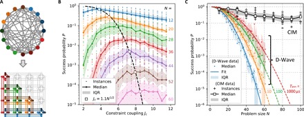
(A) Illustration of clique embedding: An arbitrary N = 16 graph is embedded into the D-Wave chimera, each spin mapped to a ferromagnetically coupled line of physical qubits (each color is a logical qubit). (B) D-Wave ground-state probability for SK model as a function of problem size N and embedding parameter J_c (annealing time T_ann = 20 μs). Shading indicates interquartile range (IQR; 25th, 75th percentile range of instances). (C) Scaling of ground-state probability for DW2Q (with optimal J_c) and Stanford CIM. D-Wave and CIM ran 20 and 10 instances per problem size, respectively.

RESULTS

SK spin-glass

As a first benchmarking problem, we consider the SK spin-glass model on a fully connected (i.e., maximally dense) graph, where the couplings J_ij = ±1 are randomly chosen with equal probability (27). Ground-state computation of the SK model is directly related to the graph partitioning problem, which is also NP-hard (43). For each problem size 2 ≤ N ≤ 61, 20 randomly chosen instances were solved on the DW2Q. We consider as a performance metric the success probability P, defined as the fraction of runs on the same instance that return the ground-state energy (we will discuss the time to solution, which requires a more thorough analysis involving optimal annealing time, in a subsequent section).

To properly benchmark the DW2Q’s performance, it is important to optimize the embedding parameter J_c, which sets the ratio of constraint couplings to logical couplings. The optimal J_c depends on the problem type and size and is found empirically. The DW2Q success probability is plotted as a function of J_c in Fig. 2B, from which we find that the optimal J_c scales roughly as N^1/2 (see Materials and Methods for details). This scaling is consistent with results published on the same class of problems with the earlier D-Wave Two quantum annealer, and it is believed to be connected to the spin-glass nature of the SK Ising problem (42). Using the optimal value of J_c, Fig. 2C shows that the performance on the D-Wave depends strongly on the single-run annealing time, with the values T_ann = (1,10,100,1000) μs plotted here. The D-Wave annealing time is restricted to the range [1,2000] μs. We observe that longer annealing times give higher success probabilities, in accordance with the expectations from the adiabatic quantum optimization approach that inspired the design of the D-Wave machine. The data fit well to a square exponential, $P=\text{exp}(-{(N/N_0^{\text{DW}})}^2)$, where the parameter $N_0^{\text{DW}}$ increases slowly, roughly logarithmically, with T_ann. For problem sizes N < 30, the results in Fig. 2C agree with an extrapolation of the benchmark data for T_ann = 20 μs reported in (42), which used an earlier processor [the 512-qubit D-Wave despite the engineering improvements that have been made in the last two generation chips (2X and 2000Q)].

The same SK instances for N = 10,20, … ,60 were solved on the CIMs hosted at Stanford University in Stanford, CA and Nippon Telegraph and Telephone Corporation (NTT) Basic Research Laboratories in Atsugi, Japan (24, 25). Additional problems with N ≥ 60 were also solved on the CIM but were too large to be programmed on the DW2Q. The two Ising machines have similar performance (see section S2 for more details). Figure 2C shows a plot of the success probability as a function of problem size: The exponential scaling for the CIM is shallower than the one given by the DW2Q performance. We note that the success probability P for the CIM scales approximately as $\text{exp}(-N/N_0^{\text{CIM}})$, where $N_0^{\text{CIM}}$ is a constant. The fact that, for the DW2Q, success probability P scales with an N² dependence in the exponential rather than N (as is the case for the CIM) leads to a marked difference in success probability between the quantum annealer and the CIM for problem sizes N ≥ 60.

MAX-CUT

We next study the DW2Q performance on MAX-CUT for both dense and sparse unweighted graphs. Unweighted MAX-CUT is the problem of finding a partition (called a cut) of the vertices V of a graph G = (V, E), where the partition is defined by two disjoint sets V₁ and V₂ with V₁ ∪ V₂ = V, and for which the number of edges between the two sets ∣{(v₁ ∈ V₁, v₂ ∈ V₂) ∈ E}∣ is maximized. Unweighted MAX-CUT is NP-hard for general graphs (2) and can be expressed as an Ising problem by setting the antiferromagnetic couplings J_ij = +1 along graph edges: H = ∑_(ij)∈Eσ_iσ_j. Thus, the problem in Fig. 1C is the same as MAX-CUT on the Möbius ladder graph. Previous CIM studies have solved MAX-CUT on problems up to size N = 2000 in experiment (24, 25, 30, 37) and N = 20,000 in simulation (29, 44).

Random unweighted MAX-CUT graphs at the phase transition (45), with an edge density of 0.5 [i.e., Erdös-Rényi graphs $G(N,\frac{1}{2})$] were tested on DW2Q for problems up to N = 61 and on the CIM for N ≤ 150. For these graphs, clique embeddings were used, but in practice, the performance did not differ from the embedding heuristic provided by the D-Wave API (21). In Fig. 3A, we show that the optimal value of the embedding coupling parameter J_c appears to be correlated with the appearance of defects in the perfect polarization state expected in logical qubits at the end of the anneal. With J_c optimized, the success probability follows the same square exponential (e^−O(N2)) trend with N as in the SK model, but the drop-off is even steeper. The CIM success probabilities are also lower than for the SK model but are now orders of magnitude higher than the DW2Q for N ≥ 40.

Fig. 3. Success probability for MAX-CUT on dense and sparse graphs.

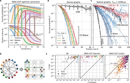
(A) D-Wave performance on dense MAX-CUT problems with (edge density of 0.5), showing that optimal performance occurs when the J_c coupling is strong enough to make it unlikely that logical qubits (chains) become “broken” (see also figs. S1 and S2). (B) D-Wave and NTT CIM success probability for dense MAX-CUT as a function of problem size (for T_soln, see fig. S6). (C) D-Wave (annealing time T_ann = 1000 μs) and NTT CIM success probability for sparse graphs of degree d = 3,4,5,7,9 and dense graphs. (D) Example of a cubic graph embedding found with the heuristic. (E) Success probability scatterplots comparing D-Wave (T_ann = 1000 μs) and CIM.

To test the effect of sparseness, we plot in Fig. 3C the performance on unweighted regular graphs of degree d = 3,4,5,7,9, where the degree of a graph is the number of edges per vertex. Despite their sparseness, MAX-CUT on these restricted graph classes is also NP-hard (46). The CIM shows no performance difference between d = 3 (cubic) and dense graphs. For DW2Q, the sparse graphs are embedded using the graph minor heuristic, which allows problems of up to size N = 200 to be embedded in the DW2Q (21). In addition, the found embeddings require significantly fewer qubits (for the sparse graphs) than the clique embeddings (compare Figs. 3D and 2A and see also fig. S3B). For cubic graphs, the DW2Q achieves slightly better performance than the CIM, while the CIM’s advantage is noticeable for d ≥ 5.

The CIM achieves similar success probabilities for cubic and dense graphs, suggesting that dense problems are not intrinsically harder than sparse ones for this class of annealer. D-Wave’s strong dependence on edge density is most likely a consequence of embedding compactness: It is known that more compact embeddings (fewer physical qubits per chain) tend to give better annealing performance after all optimization and parameter settings are considered (21). Since qubits on the D-Wave chimera graph have at most six connections, the minimum chain length is ℓ = ⌈(d − 2)/4⌉, so embeddings grow less compact with increasing graph degree (see section S3). Since degree-1 and degree-2 vertices can be pruned from a graph in polynomial time [a variant of cut-set conditioning (47)], d = 3 is the minimum degree required for NP hardness. Of NP-hard MAX-CUT instances, Fig. 3C suggests that there is only a very narrow region (d = 3,4) where D-Wave matches or outperforms the CIM in success probability; for the remainder of the graphs, the CIM dominates.

Time to solution and optimal annealing time

Although success probability is a helpful metric to understand scaling for fixed T_ann, the key computational figure of merit is the time to solution T_soln = T_ann⌈ log (0.01)/ log (1 − P)⌉. This figure multiplies the expected number of independent runs to solve a problem with 99% probability with the time of a single run, T_ann. When evaluating the time to solution of a physical annealer, it is important to optimize, as much as possible, the run parameters, in particular considering the machine’s T_soln at the optimal annealing time. This avoids a common pitfall of fixed–anneal time analysis, where if the chosen anneal time is too large, near-flat T_soln scaling for small problem sizes gives the illusion of speedup (18, 48).

In the CIM, the anneal time is set by the pump turn-on schedule and is an integer number of round trips. The experiments in this paper were conducted with T_ann = 1000 round trips, but shorter or longer times are also possible. To assess the effect of the anneal time on CIM performance, we simulate the CIM with c-number stochastic differential equations (c-SDEs) using the truncated Wigner representation (36). The algorithm, which is based on (38), is described in section S3. Figure 4A compares the performance of the experimental CIMs to the c-SDE model for dense MAX-CUT instances, indicating that the model reasonably reproduces the behavior of the experimental CIMs (similar agreement is found for SK and cubic MAX-CUT instances; see fig. S9).

Fig. 4. Time to solution for D-Wave and CIM at optimal annealing time dense MAX-CUT instances.

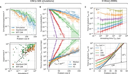
(A) CIM experimental performance versus c-SDE simulations. (B) CIM success probability and time to solution (given in terms of the number of round trips) as a function of problem size N. The effective round-trip time for the NTT CIM [(2.5N) ns; see section S2] is used to convert this figure to seconds. (C) D-Wave time to solution as a function of annealing time T_ann and problem size N. Dashed curve shows optimal CIM T_soln from (B) for comparison.

Figure 4B plots the (c-SDE) CIM success probability and time to solution (in round trips) as a function of anneal time. Consistent with the experimental results, we see an exponential scaling with N in the large-N limit [the curves are fit to P(N) = (a + (1 − a)e^bN)⁻¹, which becomes exponential for large N]. The time-to-solution plot is a series of (nearly) linear intersecting curves, where curves with shorter anneal time have a lower intercept but a larger slope. Optimizing T_soln reveals a tradeoff between the annealing time of a single run and success probability: Short anneals are preferred for small problems where the success probability is always close to unity and insensitive to the annealing time, and long anneals are preferred for large problems where the success probability dominates. Thus, the optimal anneal time depends on problem size and increases with N. Figure 4C shows the analogous D-Wave data for the same problem class (dense MAX-CUT). Here, the fixed-T_ann curves scale quadratically with N rather than linearly. The same scaling is observed in SK problems (see figs. S10 and S11).

It has been observed empirically on D-Wave quantum annealers that, for Chimera graph spin glasses, optimal time to solution scales as T_soln ∝ exp (O(N^1/2)) (18, 19, 49), while T_soln at fixed anneal times increases more steeply (18). The lower envelope of the curves in Fig. 4B can be reasonably fit to this form, suggesting a similar scaling for the CIM, although the CIM is based on an entirely different computational principle. Moreover, when solving embedded problems in quantum annealers, the optimal embedding parameters are believed to be associated with the emergence of a spin-glass phase of the embedded problem (42). Since for dense graphs the embedded problem has N_ph ∝ N² qubits, this would suggest a scaling T_soln ∝ exp(O((N²)^1/2)) = exp(O(N)), as shown in Fig. 4C. Both the CIM scaling T_soln ∝ exp(O(N^1/2)) (dashed curves in Fig. 4, B and C) and the DW2Q scaling T_soln ∝ exp(O(N)) (solid curve in Fig. 4C) are consistent with the hypothesis that a physical annealer’s time to solution (at optimal annealing time) should scale exponentially with $N_{\text{ph}}^{1/2}$, where N_ph is the number of physical qubits (or bits) required to encode the Ising problem.

We note that our claims are only suggestive, but not conclusive, of $\text{exp}(O(N_{\text{ph}}^{1/2}))$ scaling at the optimal annealing time. Only for a limited range of problem sizes (25 ≤ N ≤ 50) is the optimal annealing time accessible with the DW2Q, and the data are noisy enough that other curves would also fit the lower envelope. Thus, we caution against naïvely extrapolating these curves to large problem sizes. However, a scaling advantage for the CIM does exist at measured problem sizes, a conclusion also observed (figs. S10 and S11) for SK and cubic (i.e., d = 3) MAX-CUT instances (although the DW2Q nonetheless outperforms the CIM in absolute terms for all measured cubic MAX-CUT problems).

While the optimal–annealing time analysis is important theoretically, in realistic machines, T_ann is limited by parameter misspecification, finite temperature, and various noise sources and cannot be increased arbitrarily. Therefore, it is relevant to consider the achievable performance for practically realizable choices of T_ann. Table 1 shows the experimental times to solution for the NTT CIM (fixed T_ann = 1000 round trips) and the DW2Q (for range, T_ann ∈ [1,1000] μs). This allows a comparison of the optimal time to solution in experimentally accessible parameters, which may be more a useful benchmark for near-term annealing machines. The DW2Q outperforms the CIM by a factor of 10 to 100× at cubic MAX-CUT problems, although this factor shrinks with increasing problem size. For the SK and dense MAX-CUT problems, on the other hand, the CIM outperforms D-Wave by several orders of magnitude when N ≥ 40. For MAX-CUT, by N = 55, the factor is 10⁷, and when extrapolated to N = 100, it exceeds 10²⁰.

Table 1. Time to solution T_solnfor SK, dense MAX-CUT, and d = 3 MAX-CUT problems on D-Wave and NTT CIM (see section S2).

The annealing time for D-Wave runs was chosen (in the range [1, 1000]μs) to optimize T_soln (see section S4). All CIM data are for fixed anneal times (1000 round trips). “Factor” refers to the ratio of solution times $T_{\text{soln}}^{(\text{DW})}/T_{\text{soln}}^{(\text{CIM})}$.

SK				MAX-CUT (dense)				MAX-CUT (d = 3)
N	DW2Q	CIM	Factor	N	DW2Q	CIM	Factor	N	DW2Q	CIM	Factor
10	6.0 μs	25 μs	0.2	10	6.0 μs	25 μs	0.2	10	1.0 μs	50 μs	0.02
20	35 μs	100 μs	0.3	20	0.4 ms	100 μs	4	20	3.0 μs	100 μs	0.03
40	6.1 ms	0.4 ms	15	40	6.1 s	0.4 ms	104	50	12 μs	0.4 ms	0.03
60	1.4 s	0.6 ms	2000	55	104 s	1.2 ms	107	100	100 μs	3.3 ms	0.03
80*	(400 s)	1.8 ms	(105)	80*	(1011 s)	1.8 ms	(1013)	150	2.8 ms	22 ms	0.1
100*	(105 s)	3.0 ms	(107)	100*	(1019 s)	2.3 ms	(1021)	200	11 ms	51 ms	0.2

*D-Wave solution times extrapolated using P = e^(N/N₀)2 fits in Figs. 2C and 3B. Note that dense problems with N > 61 are not embeddable in the DW2Q.

Graph density and performance

Earlier in Fig. 3, we compared MAX-CUT on dense graphs and sparse regular graphs to show that the DW2Q’s performance depends strongly on graph sparseness. Fixing the problem size and varying the edge density, we see the same effect and can fill in the gap between sparse graphs and dense graphs. We constructed random unweighted graphs of degree d = 1,2, … , (N − 2) for each graph size N = 20,30,40,50,60. The success probabilities for DW2Q and the CIM are shown in Fig. 5A (for clarity only, N = 40 CIM data are shown). In this case, we used clique embeddings for all problems, so for a given N, all the embeddings are the same. Even with the embeddings fixed, the DW2Q finds sparse problems easier to solve than dense ones. The reason is that, consistent with (42), the optimal constraint coupling is weaker for sparse problems than for dense problems (Fig. 5B). In general, we find that J_c ∝ d for fixed N. Having a large constraint coupling could be problematic because the physical quantum annealer scales the largest coupling coefficient to the maximum coupling strength on the chip; the constraints max out this coupling and cause the logical couplings to be downscaled proportionally as $J_c^{-1}$. Thus, dense graphs have weaker logical couplings in the embedded problem, hindering the annealer’s ability to find the ground state because of parameter misspecification or “intrinsic control errors” (42, 50).

Fig. 5. Relation between edge density and annealer performance.

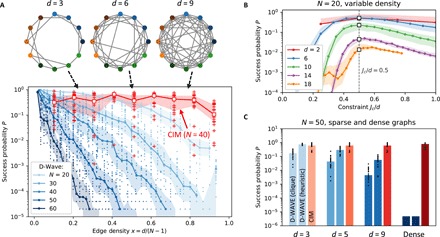
(A) Success probability as a function of edge density. Native clique embeddings used for D-Wave. Optimal embedding parameter [see subgraph (B)] is used, with T_ann = 1000 μs. (B) D-Wave success probability as a function of graph degree, showing that the optimal J_c scales as J_c ∝ d for fixed N. For fixed edge density, the N dependence was determined previously to be J_c ∝ N^3/2; see Fig. 3A. (C) Comparison of D-Wave and NTT CIM success probabilities for N = 50 using both clique embeddings and heuristically determined embeddings (T_ann = 1000 μs; dense D-Wave bars are extrapolation from e^−(N/N₀)2 fit in Fig. 3B).

The CIM has only weak dependence on the edge density x = d/(N − 1). Earlier work on N = 100 graphs (24), as well as the CIM data plotted in Fig. 3C, is consistent with this result. This suggests that the CIM has promise as a general-purpose Ising solver, achieving good performance on a large class of problems, irrespective of connectivity.

Comparing Figs. 5A and 3C, we can glean some insight regarding the effect of embedding overhead on the D-Wave quantum annealer’s performance. The heuristic embeddings in Fig. 3C are designed to minimize the overhead factor (ratio of physical qubits to logical qubits). This ratio is much larger for the native-clique embeddings, growing linearly, i.e., as O(N) (see section S1). Figure 5C compares these two D-Wave settings against the CIM at N = 50; while the CIM outperforms on all graphs with d ≥ 5, the difference between the success probabilities using clique and heuristic embeddings suggests that performance is heavily dependent on embedding overhead and the difference grows with edge density (and graph size). This illustrates an additional tradeoff in quantum annealing: poor-performing but easy-to-find embeddings versus well-performing embeddings that require substantial precomputation. This tradeoff is expected to favor the well-performing embeddings when the number of qubits (or connections) becomes large.

DISCUSSION

In conclusion, we have benchmarked the DW2Q system hosted at NASA Ames and measurement-feedback CIMs hosted at Stanford University and NTT Basic Research Laboratories, focusing on MAX-CUT problems on random graphs and SK spin-glass models, and found that the merits of each machine are highly problem dependent. Connectivity appears to be a key factor in performance differences between these machines. Problems with sparse connectivity, such as one-dimensional chains [compare (51) and (52)] and MAX-CUT on cubic graphs (Fig. 3), can be embedded into the DW2Q with little or no overhead, resulting in similar performance between the quantum annealer and the CIMs. However, the embedding overhead for dense problems such as SK is very steep, requiring O(N²) physical qubits to represent a size-N graph and resulting in large embedded problems that decrease the performance of the quantum annealer. The ability to avoid an embedding overhead likely contributes to the CIM’s performance advantage on SK models that grows exponentially with the square of the problem size. For problems of intermediate sparseness, such as MAX-CUT on regular graphs of small degree d ≥ 5, the CIM is still faster by a large factor.

Ultimately, it is overall quantities such as wall clock time or energy usage that are of practical interest. Read-in and read-out times, classical pre- and postprocessing, and energy usage must be included in a comprehensive evaluation. Both CIMs and superconducting qubit quantum annealers are in early stages of development, with these quantities currently in flux. Moreover, to beat state-of-the-art classical techniques (section S5) on the problems studied in this paper, advances will be required. D-Wave has recently implemented features allowing unconventional control of the annealing process that can significantly improve results, and as mentioned above, efforts to improve the connectivity are under way. A key question will be the extent to which these technologies can harness quantum effects for computational purposes. Signatures of entanglement have been seen in D-Wave quantum annealers, although it remains open the extent to which the computation makes use of entanglement-related effects. CIMs, already interesting as semiclassical computational devices, can, in principle, also have entanglement (53) by either building scalable all-optical couplings (30, 54) (albeit with low losses being required) or by creating entanglement in the measurement-feedback architecture, e.g., by performing entanglement swapping.

While the path forward for designing improved CIMs and quantum annealers involves many different aspects, this paper has primarily observed results that can be interpreted as being related to connectivity differences between the machines that were benchmarked. It has been conjectured often that increased internal connectivity in quantum annealers can improve performance (55, 56), and there are large projects under way to realize higher-connectivity quantum annealers [including efforts by D-Wave and the IARPA Quantum Enhanced Optimization (QEO) program (57) and Google (58)]. Our results provide strong experimental justification for this line of development.

MATERIALS AND METHODS

Sample problems

For fully connected SK and MAX-CUT on dense graphs, 20 random instances were created of each size N = 2,3, … ,61 for the D-Wave. Of these, the N = 2,10,20, … ,60 instances were also used for the CIM. An additional set of random instances were created for N = 70,80, … ,150 for the CIM using the same algorithm.

For the sparse-graph analysis, we computed regular graphs of size N = 2,4, … ,300 and degree d = 3,4, … 20, with 20 instances for each pair (N, d). The algorithm randomly assigns edges to eligible vertices until all reach the required degree (and backtracks if it gets stuck). The same algorithm was also used for the variable-density graphs: d = 1,2, … , (N − 2) for N = 20,30,40,50,60, creating 20 instances per pair (N, d).

Exact SK ground states were found with the Spin Glass Server (59), which uses BiqMac (60), an exact branch-and-bound algorithm. For SK instances of size N ≤ 100, the algorithm obtained proven ground states. For N > 100, the solver timed out before exhausting all branches (runtime T = 3000 s), so the result is not a guaranteed ground state; however, we believe that it reaches the ground state with high probability for N ≤ 150 because multiple runs of the algorithm give the same state energy and none of the CIM runs found an Ising energy lower than the Spin Glass Server result. MAX-CUT ground states for N ≤ 30 were found by brute-force search on a personal computer; for 20 ≤ N ≤ 150, a BLS algorithm was used (5). Although BLS is a heuristic solver, for N ≤ 150, it finds the ground state with nearly 100% probability, giving us high confidence that the BLS solutions are ground states. While the brute-force solver, D-Wave, and the CIM found states of equal energy to the BLS solution (if run long enough), they never found states of lower energy.

D-wave annealers

Initial D-Wave experiments were performed on the D-Wave 2X at NASA Ames Research Center and the D-Wave 2X online system at D-Wave Systems Inc. Later runs were made on the DW2Q at NASA Ames, once that machine came online. The 2X and 2000Q systems use a C12 (12 cells × 12 cells × 4 qubits) and C16 (16 × 16 × 4) Chimera, respectively. For all-to-all graphs, D-Wave 2X supports N ≤ 48 and 2000Q supports N ≤ 64 (the number is slightly smaller because of broken qubits). All N ≤ 48 runs were consistent across the three machines and with extrapolation of data in (42) from runs performed on a different set of instances on the earlier-generation machine D-Wave Two. All data reported in this paper came from the DW2Q.

Embeddings were precomputed for all problems (heuristic embeddings for sparse MAX-CUT and native clique embeddings for SK, dense MAX-CUT, and variable-density MAX-CUT) so that runs in different conditions (e.g., annealing times and constraint couplings) would use the same embeddings. For each problem type, the optimal annealing parameter J_c is found as a function of problem size N by sweeping J_c (section S1). The optimal J_c was found to be independent of the annealing time. The standard annealing schedule was used in all experiments, but the annealing time was tuned. Most instances were run 10⁴ to 10⁵ times in total depending on the observed success rate (the especially hard N ≥ 50 MAX-CUT instances were run up to 4 × 10⁶ times). Five to 10 different embeddings were used per instance, and the success probability was averaged. Spin-reversal transformations were used to avoid spurious effects. After an anneal, each logical qubit value was determined by taking the majority vote of all qubits in the chain.

In all figures, the shaded regions give the [25th, 75th] percentile range [interquartile range (IQR)] for the data. Figures 2B, 3A, and 5A show individual instances as dots and the solid line gives the median. Figures 2C, 3 (B and C), and 5B are too crowded to show D-Wave instances; the dots give medians and the smooth lines give analytic fits. For CIM data, medians and IQR are shown in Figs. 2C and 3B, while Fig. 3C only shows medians and IQR due to crowding.

Coherent Ising machine

CIM experiments were performed on the 100 OPO CIM at Ginzton Laboratory of Stanford University and the 2048 OPO CIM at NTT Basic Research Laboratories. The Stanford and NTT devices are described in (24, 25), respectively. Computation time of the Stanford CIM is 1.6 ms, which is the time for 1000 round trips of the 320-m fiber ring cavity. Since the NTT CIM processes a 2000-node problem in 5.0 ms, which is the time for 1000 round trips of the 1-km fiber ring cavity, we can solve up to ⌊2000/N⌋ problems in parallel per computation time.

The CIM’s reliable operation depends on relative phases between the OPO pulses, injection pulses, and measurement local oscillator pulses being kept stable and well calibrated. Such phase stabilization is imperfect in the experimental setups used in this study, and consequently, post-selection procedures have been applied to both the Stanford and NTT CIM experimental data. This is described in detail in section S2. Computation times have been reported in terms of annealing times; as with the DW2Q, these times exclude the time required to transfer data to and from the CIM.

SUPPLEMENTARY MATERIALS

Supplementary material for this article is available at http://advances.sciencemag.org/cgi/content/full/5/5/eaau0823/DC1

Section S1. D-Wave embeddings and J_c optimization

Section S2. CIM data and post-selection

Section S3. C-SDE simulations of CIM

Section S4. Optimal–annealing time analysis

Section S5. Performance of parallel tempering

Fig. S1. D-Wave success probability for SK problems and MAX-CUT problems of edge density 0.5 as a function of problem size N and embedding parameter J_c.

Fig. S2. MAX-CUT on graphs with an edge density of 0.5.

Fig. S3. Properties of heuristic embeddings for fixed-degree graphs.

Fig. S4. Choice of optimal coupling for sparse graphs using the heuristic embedding.

Fig. S5. Data filtering and post-selection in NTT CIM.

Fig. S6. Comparison of Stanford and NTT CIM performance for SK and dense MAX-CUT problems.

Fig. S7. Abstract schematic of measurement-feedback CIM.

Fig. S8. Simulated CIM success probability as a function of F_max for the SK, dense MAXCUT, and cubic MAX-CUT problems in this paper.

Fig. S9. Comparison of c-SDE simulations with experimental CIM data.

Fig. S10. Simulated CIM success probability and time to solution (in round trips) for SK and MAX-CUT problems.

Fig. S11. Time-to-solution analysis for D-Wave at optimal annealing time.

Fig. S12. CIM time to solution compared against the parallel tempering algorithm implemented in the Unified Framework for Optimization.

Table S1. Seven steps in a single round trip for the measurement-feedback CIM and the appropriate truncated Wigner description.

Table S2. Problem-dependent constants α and β used in the relation N₀ = α + β log₁₀(T/μs) for the success probability exponential P = e^−(N/N₀)2.

References (61–64)

REFERENCES AND NOTES

- 1.S. Rudich, A. Wigderson, Computational Complexity Theory (American Mathematical Society, 2004), vol. 10. [Google Scholar]
- 2.R. M. Karp, Complexity of Computer Computations (Springer, 1972), pp. 85–103. [Google Scholar]
- 3.Goemans M. X., Williamson D. P., Improved approximation algorithms for maximum cut and satisfiability problems using semidefinite programming. JACM 42, 1115–1145 (1995). [Google Scholar]
- 4.Kirkpatrick S., Gelatt C. D. Jr., Vecchi M. P., Optimization by simulated annealing. Science 220, 671–680 (1983). [DOI] [PubMed] [Google Scholar]
- 5.Benlic U., Hao J.-K., Breakout local search for the Max-Cutproblem. Eng. Appl. Artif. Intell. 26, 1162–1173 (2013). [Google Scholar]
- 6.Yoshimura C., Yamaoka M., Hayashi M., Okuyama T., Aoki H., Kawarabayashi K.-i., Mizuno H., Uncertain behaviours of integrated circuits improve computational performance. Sci. Rep. 5, 16213 (2015). [DOI] [PMC free article] [PubMed] [Google Scholar]
- 7.Tsukamoto S., Takatsu M., Matsubara S., Tamura H., An accelerator architecture for combinatorial optimization problems. FUJITSU Sci. Tech. J. 53, 8–13 (2017). [Google Scholar]
- 8.Sutton B., Camsari K. Y., Behin-Aein B., Datta S., Intrinsic optimization using stochastic nanomagnets. Sci. Rep. 7, 44370 (2017). [DOI] [PMC free article] [PubMed] [Google Scholar]
- 9.Parihar A., Shukla N., Jerry M., Datta S., Raychowdhury A., Vertex coloring of graphs via phase dynamics of coupled oscillatory networks. Sci. Rep. 7, 911 (2017). [DOI] [PMC free article] [PubMed] [Google Scholar]
- 10.Yin X., Sedighi B., Varga M., Ercsey-Ravasz M., Toroczkai Z., Hu X. S., Efficient analog circuits for boolean satisfiability. IEEE Trans. Very Large Scale Integr. VLSI Syst. 26, 155–167 (2018). [Google Scholar]
- 11.Tait A. N., de Lima T. F., Zhou E., Wu A. X., Nahmias M. A., Shastri B. J., Prucnal P. R., Neuromorphic photonic networks using silicon photonic weight banks. Sci. Rep. 7, 7430 (2017). [DOI] [PMC free article] [PubMed] [Google Scholar]
- 12.Farhi E., Goldstone J., Gutmann S., Lapan J., Lundgren A., Preda D., A quantum adiabatic evolution algorithm applied to random instances of an NP-complete problem. Science 292, 472–475 (2001). [DOI] [PubMed] [Google Scholar]
- 13.Kadowaki T., Nishimori H., Quantum annealing in the transverse Ising model. Phys. Rev. E 58, 5355–5363 (1998). [Google Scholar]
- 14.Santoro G. E., Tosatti E., Optimization using quantum mechanics: quantum annealing through adiabatic evolution. J. Phys. A Math. Gen. 39, R393–R431 (2006). [Google Scholar]
- 15.Boixo S., Rønnow T. F., Isakov S. V., Wang Z., Wecker D., Lidar D. A., Martinis J. M., Troyer M., Evidence for quantum annealing with more than one hundred qubits. Nat. Phys. 10, 218–224 (2014). [Google Scholar]
- 16.Santoro G. E., Martoňák R., Tosatti E., Car R., Theory of quantum annealing of an Ising spin glass. Science 295, 2427–2430 (2002). [DOI] [PubMed] [Google Scholar]
- 17.Somma R. D., Nagaj D., Kieferová M., Quantum speedup by quantum annealing. Phys. Rev. Lett. 109, 050501 (2012). [DOI] [PubMed] [Google Scholar]
- 18.Rønnow T. F., Wang Z., Job J., Boixo S., Isakov S. V., Wecker D., Martinis J. M., Lidar D. A., Troyer M., Defining and detecting quantum speedup. Science 345, 420–424 (2014). [DOI] [PubMed] [Google Scholar]
- 19.Albash T., Lidar D. A., Demonstration of a scaling advantage for a quantum annealer over simulated annealing. Phys. Rev. X 8, 031016 (2018). [Google Scholar]
- 20.Choi V., Minor-embedding in adiabatic quantum computation: I. The parameter setting problem. Quantum Inf. Process 7, 193–209 (2008). [Google Scholar]
- 21.J. Cai, W. G. Macready, A. Roy, A practical heuristic for finding graph minors. arXiv:1406.2741 [quant-ph] (10 June 2014).
- 22.Choi V., Minor-embedding in adiabatic quantum computation: II. minor-universal graph design. Quantum Inf. Process 10, 343–353 (2011). [Google Scholar]
- 23.Klymko C., Sullivan B. D., Humble T. S., Adiabatic quantum programming: Minor embedding with hard faults. Quantum Inf. Process 13, 709–729 (2014). [Google Scholar]
- 24.McMahon P. L., Marandi A., Haribara Y., Hamerly R., Langrock C., Tamate S., Inagaki T., Takesue H., Utsunomiya S., Aihara K., Byer R. L., Fejer M. M., Mabuchi H., Yamamoto Y., A fully programmable 100-spin coherent Ising machine with all-to-all connections. Science 354, 614–617 (2016). [DOI] [PubMed] [Google Scholar]
- 25.Inagaki T., Haribara Y., Igarashi K., Sonobe T., Tamate S., Honjo T., Marandi A., McMahon P. L., Umeki T., Enbutsu K., Tadanaga O., Takenouchi H., Aihara K., Kawarabayashi K.-i., Inoue K., Utsunomiya S., Takesue H., A coherent Ising machine for 2000-node optimization problems. Science 354, 603–606 (2016). [DOI] [PubMed] [Google Scholar]
- 26.Barahona F., On the computational complexity of Ising spin glass models. J. Phys. A Math. Gen. 15, 3241–3253 (1982). [Google Scholar]
- 27.Kirkpatrick S., Sherrington D., Solvable model of a spin-glass. Phys. Rev. Lett. 35, 1792–1796 (1975). [Google Scholar]
- 28.R. W. Boyd, Nonlinear Optics (Academic Press, 2003). [Google Scholar]
- 29.Wang Z., Marandi A., Wen K., Byer R. L., Yamamoto Y., Coherent Ising machine based on degenerate optical parametric oscillators. Phys. Rev. A 88, 063853 (2013). [Google Scholar]
- 30.Marandi A., Wang Z., Takata K., Byer R. L., Yamamoto Y., Network of time-multiplexed optical parametric oscillators as a coherent Ising machine. Nat. Photonics 8, 937–942 (2014). [Google Scholar]
- 31.Takesue H., Inagaki T., 10 GHz clock time-multiplexed degenerate optical parametric oscillators for a photonic Ising spin network. Opt. Lett. 41, 4273–4276 (2016). [DOI] [PubMed] [Google Scholar]
- 32.D. F. Walls, G. J. Milburn, Quantum Optics (Springer Science & Business Media, 2007). [Google Scholar]
- 33.Milburn G., Walls D., Production of squeezed states in a degenerate parametric amplifier. Opt. Commun. 39, 401–404 (1981). [Google Scholar]
- 34.Drummond P., McNeil K., Walls D., Non-equilibrium transitions in sub/second harmonic generation. J. Mod. Opt. 28, 211–225 (1981). [Google Scholar]
- 35.Wu L.-A., Kimble H. J., Hall J. L., Wu H., Generation of squeezed states by parametric down conversion. Phys. Rev. Lett. 57, 2520–2523 (1986). [DOI] [PubMed] [Google Scholar]
- 36.Kinsler P., Drummond P. D., Quantum dynamics of the parametric oscillator. Phys. Rev. A 43, 6194–6208 (1991). [DOI] [PubMed] [Google Scholar]
- 37.Takata K., Marandi A., Hamerly R., Haribara Y., Maruo D., Tamate S., Sakaguchi H., Utsunomiya S., Yamamoto Y., A 16-bit coherent Ising machine for one-dimensional ring and cubic graph problems. Sci. Rep. 6, 34089 (2016). [DOI] [PMC free article] [PubMed] [Google Scholar]
- 38.Hamerly R., Inaba K., Inagaki T., Takesue H., Yamamoto Y., Mabuchi H., Topological defect formation in 1D and 2D spin chains realized by network of optical parametric oscillators. Int. J. Mod. Phys. B 30, 1630014 (2016). [Google Scholar]
- 39.Clements W. R., Renema J. J., Wen Y. H., Chrzanowski H. M., Kolthammer W. S., Walmsley I. A., Gaussian optical Ising machines. Phys. Rev. A 96, 043850 (2017). [Google Scholar]
- 40.Yamamoto Y., Aihara K., Leleu T., Kawarabayashi K.-i., Kako S., Fejer M., Inoue K., Takesue H., Coherent Ising machines—Optical neural networks operating at the quantum limit. npj Quantum Inf. 3, 49 (2017). [Google Scholar]
- 41.Boothby T., King A. D., Roy A., Fast clique minor generation in chimera qubit connectivity graphs. Quantum Inf. Process 15, 495–508 (2016). [Google Scholar]
- 42.Venturelli D., Mandrà S., Knysh S., O’Gorman B., Biswas R., Smelyanskiy V., Quantum optimization of fully connected spin glasses. Phys. Rev. X 5, 031040 (2015). [Google Scholar]
- 43.Fu Y., Anderson P. W., Application of statistical mechanics to NP-complete problems in combinatorial optimisation. J. Phys. A Math. Gen. 19, 1605–1620 (1986). [Google Scholar]
- 44.Haribara Y., Utsunomiya S., Yamamoto Y., Computational principle and performance evaluation of coherent Ising machine based on degenerate optical parametric oscillator network. Entropy 18, 151 (2016). [Google Scholar]
- 45.Coppersmith D., Gamarnik D., Hajiaghayi M., Sorkin G. B., Random max sat, random max cut, and their phase transitions. Random Struct. Algoritms 24, 502–545 (2004). [Google Scholar]
- 46.P. Alimonti, V. Kann, Hardness of approximating problems on cubic graphs, in Proceedings of the Third Italian Conference on Algorithms and Complexity (CIAC), Berlin, Heidelberg, 12 to 14 March 1997, pp. 288–298. [Google Scholar]
- 47.R. Dechter, J. Pearl, The Cycle-Cutset Method for Improving Search Performance in AI Applications (University of California, Computer Science Department, 1986). [Google Scholar]
- 48.C. C. McGeoch, W. Bernoudy, J. King, Comment on “Scaling advantages of all-to-all connectivity in physical annealers: The Coherent Ising Machine vs D-Wave 2000Q”. arXiv:1807.00089 [quant-ph] (29 June 2018).
- 49.Mandra S., Katzgraber H. G., A deceptive step towards quantum speedup detection. Quantum Sci. Technol. 3, 04LT01 (2018). [Google Scholar]
- 50.D-Wave Systems Inc., Technical description of the D-Wave quantum processing unit, Part of D-Wave API documentation (2016).
- 51.Gardas B., Dziarmaga J., Zurek W. H., Zwolak M., Defects in quantum computers. Sci. Rep. 8, 4539 (2018). [DOI] [PMC free article] [PubMed] [Google Scholar]
- 52.Inagaki T., Inaba K., Hamerly R., Inoue K., Yamamoto Y., Takesue H., Large-scale Ising spin network based on degenerate optical parametric oscillators. Nat. Photonics 10, 415–419 (2016). [Google Scholar]
- 53.Maruo D., Utsunomiya S., Yamamoto Y., Truncated Wigner theory of coherent Ising machines based on degenerate optical parametric oscillator network. Phys. Scr. 91, 083010 (2016). [Google Scholar]
- 54.Shen Y., Harris N. C., Skirlo S., Prabhu M., Baehr-Jones T., Hochberg M., Sun X., Zhao S., Larochelle H., Englund D., Soljačić M., Deep learning with coherent nanophotonic circuits. Nat. Photonics 11, 441–446 (2017). [Google Scholar]
- 55.Katzgraber H. G., Hamze F., Andrist R. S., Glassy chimeras could be blind to quantum speedup: Designing better benchmarks for quantum annealing machines. Phys. Rev. X 4, 021008 (2014). [Google Scholar]
- 56.Rieffel E. G., Venturelli D., O’Gorman B., Do M. B., Prystay E. M., Smelyanskiy V. N., A case study in programming a quantum annealer for hard operational planning problems. Quantum Inf. Process 14, 1–36 (2015). [Google Scholar]
- 57.Weber S., Samach G., Rosenberg D., Yoder J., Kim D., Kerman A., Oliver W., Hardware considerations for high-connectivity quantum annealers. Bull. Am. Phys. Soc. (2018). [Google Scholar]
- 58.Y. Chen, C. Quintana, D. Kafri, A. Shabani, B. Chiaro, B. Foxen, Z. Chen, A. Dunsworth, C. Neill, J. Wenner, H. Neven, J. Martinis; Google Quantum Hardware Team, Progress towards a small-scale quantum annealer I: Architecture. Bull. Am. Phys. Soc. (2017).
- 59.F. Liers, M. Jünger, Spin glass server; http://informatik.uni-koeln.de/spinglass/.
- 60.Rendl F., Rinaldi G., Wiegele A., Solving Max-Cut to optimality by intersecting semidefinite and polyhedral relaxations. Math. Program. 121, 307–335 (2010). [Google Scholar]
- 61.D-Wave Systems Inc., Chimera embedding (2016); https://github.com/dwavesystems/chimera-embedding.
- 62.A. D. King, W. Bernoudy, J. King, A. J. Berkley, T. Lanting, Emulating the coherent Ising machine with a mean-field algorithm. arXiv:1806.08422 [quant-ph] (21 Jun 2018).
- 63.Mandrà S., Katzgraber H. G., Thomas C., The pitfalls of planar spin-glass benchmarks: raising the bar for quantum annealers (again). Quantum Sci. Technol. 2, 038501 (2017). [Google Scholar]
- 64.Mandrà S., Zhu Z., Wang W., Perdomo-Ortiz A., Katzgraber H. G., Strengths and weaknesses of weak-strong cluster problems: A detailed overview of state-of-the-art classical heuristics versus quantum approaches. Phys. Rev. A 94, 022337 (2016). [Google Scholar]
Associated Data
This section collects any data citations, data availability statements, or supplementary materials included in this article.