

Abstract
Two-node attractor networks are flexible models for neural activity during decision making. Depending on the network configuration, these networks can model distinct aspects of decisions including evidence integration, evidence categorization, and decision memory. Here, we use attractor networks to model recent causal perturbations of the frontal orienting fields (FOF) in rat cortex during a perceptual decision-making task (Erlich, Brunton, Duan, Hanks, & Brody, 2015). We focus on a striking feature of the perturbation results. Pharmacological silencing of the FOF resulted in a stimulus-independent bias. We fit several models to test whether integration, categorization, or decision memory could account for this bias and found that only the memory configuration successfully accounts for it. This memory model naturally accounts for optogenetic perturbations of FOF in the same task and correctly predicts a memory-duration-dependent deficit caused by silencing FOF in a different task. Our results provide mechanistic support for a “postcategorization” memory role of the FOF in upcoming choices.
1. Introduction
Perceptual decision making is a commonly studied behavioral paradigm because it requires multiple types of computations: sensory processing, executive functions, and motor responses. Several recent studies have examined the role of a rat cortical area known as the frontal orienting fields (FOF) in decision making and short-term memory (Erlich, Bialek, & Brody, 2011; Erlich, Brunton, Duan, Hanks, & Brody, 2015; Hanks et al., 2015; Kopec, Erlich, Brunton, Deisseroth, & Brody, 2015). These studies have used two different tasks to ask separate questions about evidence integration, decision making, and short-term memory. During the Poisson clicks task, rats were trained to integrate noisy evidence informing them which choice, left or right, would be rewarded (Brunton, Botvinick, & Brody, 2013; Erlich et al., 2015; Hanks et al., 2015). During the memory-guided orienting (MGO) task, rats were presented with a nonnoisy auditory stimulus indicating a reward location, and then they were required to wait during a delay period before making their choice (Erlich et al., 2011; Kopec et al., 2015). During both tasks, performance can be assessed via a psychometric curve that displays the relationship between trial difficulty and the animal’s choice.
In order to investigate the causal role of the FOF in these cognitive tasks, recent studies have used a pharmacological agent, muscimol, to reversibly inactivate the FOF. On both tasks, unilateral inactivation of the FOF produced an ipsilateral bias (toward the side of infusion). This bias is evident as a mostly vertical scaling of the psychometric curve (see Figure 1). A vertical scaling is highly unusual, as it means that the rat’s bias was independent of trial difficulty. Easy trials were biased (scaled) by the same percentage as hard trials. Vertical scaling is most evident in the change in the asymptotes of the psychometric curve. An alternative type of bias, and one that is readily observed by perturbing evidence accumulation models, is a horizontal shift of the psychometric curve (Hanks, Ditterich, & Shadlen, 2006). In a horizontal shift, the midpoint of the curve moves laterally, while the curve has the same asymptotic behavior. A horizontal shift means easy trials are less biased than hard trials.
Figure 1:
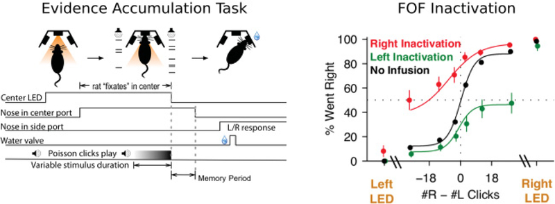
Cortical inactivation produces an ipsilateral bias during decision making. Description of the behavioral data modeled in this study. (Left) Task schematic of an evidence accumulation task (adapted from Brunton et al., 2013; Erlich et al., 2015; Hanks et al., 2015). Rats enter a center nose port and hear Poisson-generated clicks from both a speaker to their left and a speaker to their right. After the click trains have ended, the rats must enter a nose port on the side that played the greater total number of clicks to get a reward. (Right) Muscimol infusion into the frontal orienting fields produces an ipsilateral bias. Sensory instructed trials in which a visual sensory signal (LED turning on in the reward port) indicates which of the two side ports is the correct choice, are not biased after FOF inactivation (left/right LED). (Reproduced from Erlich et al., 2015.)
To understand the origin of this ipsilateral bias, Erlich et al. (2015) performed an analysis of perturbations to behavioral-level accumulation models that describe rat performance on the evidence accumulation task. They concluded that the best description of the bias was postcategorization bias, which was formulated as a directional lapse rate. This term describes the idea that on a fraction of trials, the animal responds toward the inactivated side regardless of the evidence. Lapses are so called because they are often assumed to come from a lapse of attention (Wichmann & Hill, 2001), but may have more interesting and nuanced sources (Scott, Constantinople, Erlich, Tank, & Brody, 2015). The term captures the qualitative pattern of the data but does not indicate a neural mechanism that would create postcategorization bias.
Optogenetic inactivation of the FOF was also found to produce an ipsilateral bias, on both behavioral tasks (Hanks et al., 2015; Kopec et al., 2015). During the evidence accumulation task, behavior was biased only when the inactivation period included the end of the evidence period. The interpretation given by Hanks et al. (2015) was that the FOF may be involved in “reading out” the decision from the accumulated evidence but not integrating the evidence itself. Consistent with pharmacological inactivations, the data were best fit by a model with a postcategorization bias term (Hanks et al., 2015). During the MGO task, Kopec et al. (2015) used fast timescale optogenetic inactivation and again found an ipsilateral bias. The changes relative to controls in the psychometric curve during optogenetic inactivation showed a smaller bias than with pharmacological inactivation and did not display the clear vertical scaling. The origin of these differences between optogenetic and pharmacological inactivations in the MGO task remains unclear. Kopec et al. (2015) fit a mutual inhibition attractor model to the perturbation data from their MGO task and found that it was consistent with several aspects of the data.
Such mutual inhibition models have previously been used to model short-term memory and decision making (Machens, Romo, & Brody, 2005; Wong & Wang, 2006). Consisting of two neural population variables, they are simple yet surprisingly flexible at implementing many cognitive computations. At the root of their flexibility is the ability to implement many distinct nonlinear computations with low-dimensional dynamics (Machens et al., 2005). Recent studies have suggested that neural populations compute via effective low-dimensional dynamics, including both the PFC (Mante, Sussillo, Shenoy, & Newsome, 2013) and the hippocampus (Yoon et al., 2013). Theoretical studies of large recurrent network models have also found effective low-dimensional dynamics, including both trained networks (Sussillo & Barak, 2012) and random unstructured networks (Aljad-eff, Renfrew, Vegue, & Sharpee, 2016). Mutual inhibition models implement low-dimensional dynamics without the complications of larger network details. They can be derived from spiking network models through the use of simplifying mean field reductions (Wong & Wang, 2006). When tuned correctly, they can also be reduced to a drift diffusion model that describes optimal integration (Bogacz, Brown, Moehlis, Holmes, & Cohen, 2006). Given that these models can tractably perform all three functions of decision making, they are a natural tool to examine the possible roles of the FOF during evidence integration, decision categorization, and short-term memory.
Here, using mutual inhibition models, we set out to ask (1) how postcategorization bias could be implemented in a neural circuit; (2) whether this bias was consistent with the FOF integrating evidence, categorizing accumulated evidence, or maintaining a decision memory in the Poisson clicks task; and (3) whether the attractor model used to describe data from the MGO task (Kopec et al., 2015) could also explain data from the Poisson clicks task. We will show that a mutual inhibition neural circuit model similar to that used by Kopec et al. (2015) can indeed recreate postcategorization bias in the Poisson clicks task, but only when it is used to maintain choice memory, not when it is involved in evidence integration or decision categorization.
2. Results
We considered three distinct computational stages of decision making that might explain the results of pharmacological inactivation of the FOF during the evidence accumulation task: evidence integration, categorization of accumulated evidence into a decision, and decision memory. During the evidence integration stage, transient noisy evidence must be integrated over time to produce the accumulated evidence value. The accumulated evidence has been the primary focus of study in recent papers (Brunton et al., 2013; Hanks et al., 2015; Scott et al., 2015). In the categorization stage, the accumulated evidence value is evaluated to produce a binary choice: left or right. In the decision memory stage, a categorized choice must be maintained. We did not consider a motor role in producing these biases because FOF inactivation did not produce a bias in sensory instructed trials (see Figure 1, “left/right LED,” and Erlich et al., 2015). Our conceptual model assumes these three stages operate in a serial fashion (see Figure 2).
Figure 2:
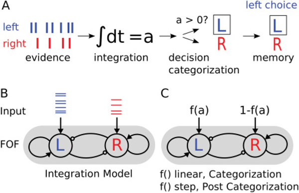
Conceptual stages of decision making. (A) We consider three stages of decision making that might be perturbed during FOF inactivation: integration, decision categorization, and decision memory. In this cartoon, seven clicks are presented on the left and four on the right. The evidence is integrated, categorized into a go-left trial, and the decision is remembered. (B) Schematic of the integration model. Two nodes represent populations of neurons that self-excite and have cross-inhibition. Each node gets feedforward input consisting of the evidence click trains. (C) Schematic of the categorization and postcategorization models. The accumulated evidence a is passed through a thresholding function f () that has a parameter g describing how “soft” or “hard” the thresholding is and then used as inputs into the model. In the categorization model, the parameter g is fixed such that the function f () is linear, so that categorization of the value of a into a left or right choice occurs within or after the mutual inhibition model. In the postcategorization model, the parameter g = 0; then f () becomes the Heaviside step function, indicating the choice has already been categorized before entering the mutual inhibition model. When fitting the postcategorization model, we allowed g to be a free parameter in order to fit the degree to which inputs have already been categorized.
Mutual inhibition models can be tuned to implement all three of these computations (Machens et al., 2005; Wong & Wang, 2006). To evaluate whether the FOF could be implementing these computations, we fit mutual inhibition models to perform each of these computations with and without inactivations. Our model is a simplification of Kopec et al. (2015), Machens et al. (2005), and Wong and Wang (2006). It consists of two nodes that represent the average activity of a neural population. Each node has dynamics according to
| (2.1) |
| (2.2) |
The variable Ui represents the internal state of each population. The variable Vi represents the external activation of each population and is bounded between 0 and 1. Each population gets independent additive white noise, W, with variance given by σ2. The two populations have a time constant τ, which was set to 100 msec. The self-excitation has strength M, and the cross-inhibition has strength I.
To model a unilateral muscimol inactivation, the output of one node V is scaled by h, the inactivation fraction (0 ≤ h ≤ 1). Scaling the output of a node represents part of the neural population being inactivated, creating a weakened population signal. Allowing for a partial inactivation of a neural population could reflect either incomplete inactivation of the FOF hemisphere or the FOF operating as part of a larger distributed circuit (Kopec et al., 2015). Due to the decussation of motor pathways from the brain to the body, we simulate an inactivation of the right hemisphere of the rat’s brain by inactivating the left node of our model. This produces a bias toward right choices, consistent with the ipsilateral bias in the data. In terms of equation 2.2, a right hemisphere inactivation has hL = h and hR = 1, while a left hemisphere inactivation has hR = h and hL = 1, and control trials have hR = hL = 1.
The external input to each node Exi is dependent on the current epoch within each trial. During the stimulus period, each node gets a constant background node-independent input B plus an additional node-dependent input ø scaled by Ecue;
| (2.3) |
The input ø is either the auditory clicks, the accumulated evidence, or the categorized decision depending on whether the integration, categorization, or postcategorization model is being considered. During the memory period, we have no external inputs:
| (2.4) |
The value of øi, will represent either the noisy evidence, the accumulated evidence, or the categorized decision. At the end of each trial, we read out the model’s choice by determining which node has greater activity. The control and inactivation data were fit simultaneously, with the inactivation fraction h = 1 during simulation of control trials. The parameters M, I, σ, B, Ecue, h, and g (introduced below) were fit to the data.
2.1. Integration Model.
The first computational stage the FOF might implement is evidence integration. The mutual inhibition model can integrate evidence by setting
| (2.5) |
where δi,t are delta functions at the times of each click on the left or right side. The model was fit to the data by maximizing the likelihood of observing the rat’s choice on each trial in the data set. The length of the memory period on each trial was the duration from when the center light went off, indicating to the rat the evidence period had ended, and when the rat left the center nose poke. The memory period was about 60 msec on average. The model was also fit with no memory period on each trial, and with a 100 msec memory period on each trial, all of these models fit the data poorly. When fit to the control data alone, the integration model produces a psychometric curve similar to the data (see supplementary Figure 1). However, when inactivation data are included in the model fitting, the model cannot produce the same type of vertical scaling seen in the data (see Figure 3). The integration model cannot produce the correct type of bias because it must encode graded, rather than categorical, information. To perform accurate integration, the information in the network must be encoded in a graded manner such that a click on each side can be accurately added to previous clicks. Inactivation of a network with graded information produces biases that make some clicks weaker. The model is unable to balance this constraint with the difficulty-independent bias in the data and is unable to fit the data. The failure of the integration model suggests that inactivation of the FOF is not perturbing an evidence integration process.
Figure 3:
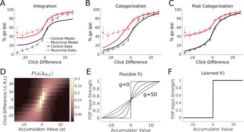
The integration model fails to fit the data; The postcategorization model fits the data well. (A-C) Solid lines indicate model behavior. Dashed lines indicate rat data. Data from left and right inactivations from all rats have been transformed into one “meta-rat” data set. Ipsilateral refers to the side of muscimol infusion relative to choice. Error bars on data indicate 95% confidence intervals. (A) The best-fit integration model on a test set. (B) The categorization model (setting g = 50) fails to match the bias on easy contralateral trials. (C) The best-fit postcategorization model (fitting g) on a test set matches both the control and perturbed psychometric curves. (D) A visualization of P(a|ΔR,L). For every click difference, the average distribution of accumulator values predicted by the accumulation model is shown as a heat map. (E) Possible thresholding functions. Changing g allows the threshold function f () to vary from linear to the Heaviside function. Five example values of g are plotted here: 0,2, 5,10, and 50. The minimum and maximum accumulation values used to bound the domain of f () were determined by the accumulation model and fit to data. (F) The learned threshold function f () for the memory model is a steep sigmoid function (g < 1). This indicates the input into the model is already categorical, and thus the FOF supports a postcategorization memory.
2.2. Categorization and Postcategorization Models.
Next we consider how the FOF might categorize accumulated evidence or maintain a categorized choice. For both of these roles, the input to each node will be a function of the accumulated evidence a:
| (2.6) |
There are many possible functions f (), but we will add several restrictions on this function. First, we restrict f () such that it has range [0, 1] and domain [amin, amax], determined by the largest and smallest accumulated evidence values the rats experience. Second, we require f () to be monotonically increasing, which implies f (amin) = 0 and f (amax) = 1. Third, we require that f() can be parameterized such that it can move smoothly between a straight line over its domain and the Heaviside step function. This parameterization allows the model-fitting process to determine that degree to which input into the network is graded (linear function) or categorical (Heaviside step function). One function that can satisfy these conditions is tanh scaled appropriately:
| (2.7) |
As f () returns a linearly graded value on the domain between amin and amax, creating the categorization model. In this setting, the model categorizes the accumulated evidence into a binary left or right decision and then maintains that memory. As g → 0, f () becomes the Heaviside function, creating the postcategorization model. In this setting, the model performs only a decision memory role, as the input is already formed into a decision. Intermediate values of g can create partially categorized inputs. We will refer to f () as the thresholding function. Introducing f () allows us to fit the degree of categorization in the input to the FOF.
The model described thus far computes the probability of a choice right (or left) as a function of the accumulated evidence, P(R|a). However, in order to fit the models to the psychometric curves, we need to compute the probability the model will choose right (or left) given a click difference: P(R|ΔR,L). We could do this directly by using the click difference as the accumulated evidence: a = ΔR,L. However, this approach assumes perfect integration and ignores the noise of integration. Previous studies have demonstrated and quantified the impact of sensory noise in evidence integration (Brunton et al., 2013; Scott et al., 2015). To respect the noisy integration process, we introduce a latent accumulation variable:
| (2.8) |
We can determine P(a|ΔR,L) by use of a previously developed evidence accumulation model (Brunton et al., 2013). This accumulation model gives us a moment-by-moment estimate of the accumulation variable given the trial’s evidence, The accumulation model outputs a distribution over possible a values, reflecting model uncertainty To construct P(a|ΔR,L), we used parameters for the accumulation model taken from the fit of the model in Erlich et al. (2015) to the control data set. The accumulation model was then used to generate a distribution of a values at the end of each trial. All trials with the same click difference were averaged to produce P(a|ΔR,L). The best-fit parameters of the accumulation model included sticky bounds on integration at a = ±15. We can compute P(R\a) by simulating the mutual inhibition model with with −15 ≤ a ≤ 15. The sticky bounds also determined the domain of the threshold function f (). Combining these two terms, we can estimate the probability of our model’s behavior given a click difference on each trial. Practically, we discretize and bin a:
| (2.9) |
Our results are insensitive to particular bin sizes for these values. The same bin sizes and the same values for P(a|ΔR,L) were used in all the model fits presented. The model was fit by maximizing the likelihood of observing the data given the model. The model was simulated with a 1 evidence period and a 100 ms memory period.
We fit the categorization model by fixing g = 50, which is large enough to create a linear input function (see Figure 3). A linear input function requires that the model must categorize graded inputs into a decision. The categorization model fits better than the integration model but still fails to qualitatively match the bias in the psychometric curve (see Figure 3). This suggests that FOF inactivations do not perturb the decision categorization process.
We fit the postcategorization model by allowingg to be a parameter in the fitting process. The maximum likelihood estimate of g is 0.167 ± 0.18, which creates a steep sigmoid function (see Figure 3, bottom right). In addition, the best-fitting model includes significant mutual inhibition (I: 7.04 ± 0.027). The best-fit model produces a psychometric curve that matches the data well (see Figure 3, top right). This suggests that perturbing the FOF disrupts a postdecision binary memory because the bistable attractor model can match the FOF bias when perturbed.
2.3. Postcategorization Is the Best-Fitting Model.
To quantify the performance of each model, we computed the Bayesian information criterion (BIC). BIC allows for model comparison between models with a different number of parameters by penalizing models with more parameters, favoring more parsimonious models. BIC punishes additional parameters more harshly than other model comparison tools like AIC. The integration and categorization models have 6 parameters, while the postcategorization model has 7 parameters. The categorization and postcategorization models have an additional 7 parameters from the accumulation model used to compute P(a|ΔR,L), for a total of 13 and 14 parameters, respectively. A smaller BIC value indicates a better fit. We can compare models by examining the ΔBIC relative to the best-fit model: Post Categorization ΔBIC 0, Categorization ΔBIC +274, Integration ΔBIC +640. BIC values were computed using two-fold cross-validation (see section 4 for more details). Despite the penalty for more parameters, the postcategorization model significantly outperforms the integration model.
Table 1 shows the best-fit parameters for each of the models, as well as parameter uncertainty. Parameter uncertainty for each model was estimated using the Laplace approximation, which approximates the local likelihood landscape with a multidimensional gaussian (Daw, 2011). The eigenvector associated with the largest eigenvalue of the approximated covariance matrix tells us the “sloppiest” direction in parameter space, for which the model is the least constrained (Brown & Sethna, 2003). In the postcategorization model, 95% of the total variance (the sum of covariance matrix eigenvalues) in our parameters lies along the vector associated with the parameter g. Due to g’s nonlinear implementation, the model is relatively insensitive to this parameter near g = 0. All other eigenvalues were relatively small and within one order of magnitude of each other, suggesting all other directions in parameter space were equally “stiff.” This analysis suggests that there are not significant trade-offs in parameter space that would replicate our model’s behavior.
Table 1:
Maximum Likelihood Parameters and the Standard Error for Each Parameter.
| Parameter | Integration | Categorization | Postcategorization | Bilateral |
|---|---|---|---|---|
| M | 0.01 ± 0.01 | 3.25 ± 0.19 | 2.50 ± 0.016 | 2.66 ± 0.19 |
| I | 8.18 ± 0.19 | 7.51 ± 0.14 | 7.04 ± 0.027 | 9.81 ± 0.10 |
| B | 1.44 ± 0.32 | 2.60 ± 0.076 | 4.07 ± 0.014 | 3.54 ± 0.10 |
| Ecue | 4.78 ± 0.10 | 8.83 ± 0.082 | 3.49 ± 0.016 | 9.64 ± 0.45 |
| σ 2 | 2.00 ± 0.001 | 0.42 ± 0.025 | 1.97 ± 0.0070 | 9.32 ± 0.098 |
| h | 0.58 ± 0.013 | 0.91 ± 0.0037 | 0.693 ± 0.0073 | 0.56 ± 0.029 |
| g | - | 50 (fixed) | 0.168 ± 0.18 | 1.62 ± 0.23 |
| hbi-R | - | - | - | 0.43 ± 0.052 |
| hbi-L | - | - | - | 0.33 ± 0.054 |
| ΔBIC | +640 | +274 | 0 | - |
The categorization model transforms a graded signal into a categorical decision by the use of bistable dynamics. The postcategorization model works by implementing bistable dynamics that encode an already categorized signal. Because the thresholding function f () is a steep sigmoid function, the information in the model is categorical, reflecting only the upcoming choice, not the evidence for that choice. To understand the bistable dynamics in the postcategorization model, we computed phase plane diagrams and a bifurcation diagram with respect to inactivation strength (see Figure 4). When one of the nodes is partially inactivated by muscimol, the stable fixed point weakens, allowing noise to more easily corrupt the stored memory.
Figure 4:
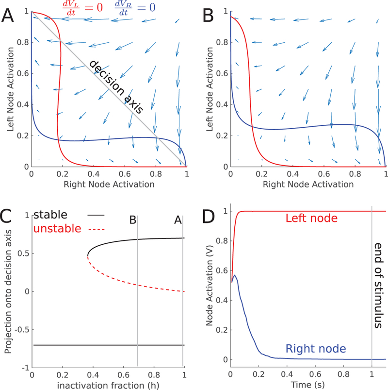
Dynamics of postcategorization model (A) Phase plane diagram for the postcategorization model during the memory period without inactivation. Solid lines are the nullclines of the external variables. (B) Same as panel A, but with partial muscimol inactivation of the left node. (C) Bifurcation diagram with respect to the inactivation fraction h. Near h = 0.35, the left attractor disappears in a saddle node bifurcation. Lines marked A and B show the parameter values used in panels A and B. (D) Mean activation of each node during a Go-Left trial (a = −10).
We highlight two properties of the post-categorization model that are consistent with the data. First, a direct result of the categorical encoding is that bias strength during an inactivation is independent of trial difficulty Conditioned on initial decision choice, easy trials are biased with the same probability as hard trials. This happens because information about trial difficulty is never present in the mutual inhibition model. This is the striking feature of the data, and the one we set out to model. Second, the categorical encoding of the accumulated evidence variable (see Figure 4D) is consistent with analysis of spike trains recorded from the FOF that found the FOF encodes evidence in a more categorical manner than other brain regions (Hanks et al., 2015). In order to quantify the categorical encoding in the FOF, we constructed tuning curves for the post-categorization model, using the method developed by Hanks et al. (2015; see Figure 5A). We fit a sigmodial curve to the tuning curve to find the slope of the curve at a = 0. Our model has a slope of 0.133 compared to the FOF population average of 0.158 ± 0.015 reported by Hanks et al. (2015). The post-categorization model categorically encodes the accumulated evidence, in a manner similar to the FOF. Our model is also supported by data from temporally precise optogenetic inactivations and muscimol inactivations with long memory periods.
Figure 5:
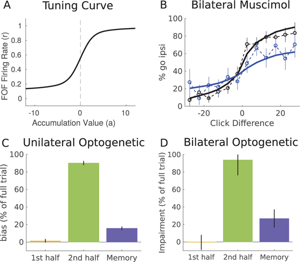
Properties of postcategorization model. (A) Tuning curve for FOF model showing the firing rate as a function of the accumulation value. Constructed using the method developed in Hanks et al. (2015). The slope of the tuning curve at a = 0 is 0.133, comparable to the FOF population average of 0.158 ± 0.015 reported in Hanks et al. (2015). (B) Psychometric curve for bilateral muscimol inactivations of the FOF. The model (solid line) is able to match the psychometric curves from the data (dashed). The model was fit simultaneously to both unilateral and bilateral data sets. (C, D) The postcategorization model was simulated using temporally precise inactivations, mimicking opto-genetic experiments. Error bars show model variability over repeated sampling of trajectories. Three trial epochs were inactivated: the first and second half of the evidence period (yellow, green) and the memory period (blue). All trials had a 1 s evidence period. Memory period duration was 100 msec. Inactivation effect is shown as the percentage of bias on model full trial inactivation. (C) Unilateral inactivation produces an ipsilateral bias. (D) Bilateral inactivation, showing average impairment on each side.
2.4. Postcategorization Model Matches Bilateral Muscimol Inactivation Psychometrics.
In addition to the unilateral inactivations focused on in our study, Erlich et al. (2015) also performed bilateral inactivations. When the FOF was infused bilaterally with muscimol, the psychometric curve had both the upper and lower asymptotes move closer together. To assess if the postcategorization model was consistent with the bilateral results, we fit the postcategorization model simultaneously to the unilateral and bilateral inactivation data. We modeled the inactivations in the same manner as before by scaling the output of each node V by an inactivation fraction h. We allowed a different inactivation strength during unilateral inactivations and bilateral inactivations. In addition, during bilateral inactivations, we allowed each node to have a different inactivation fraction (hR and hL can be different). This created three inactivation parameters. The model was able to produce psychometric curves that match both the bilateral and unilateral inactivations (see Figure 5B). The postcategorization model matches the bilateral inactivation psychometric curve by an increased lapse rate in both directions and the unilateral inactivation curve by a unidirectional lapse rate.
Using a behavioral model, Erlich et al. (2015) found that the bilateral inactivation data, unlike the unilateral data, were better described by a change to the integration time constant than an increased lapse rate. Our model does not produce a change in the integration time constant by itself. Erlich et al. (2015) also hypothesized that a short time constant integration circuit becomes dominant when the FOF is bilaterally inactivated. Our model could be consistent with this hypothesis, but since it involves an alternate circuit and pathway, it lies outside the scope of the current work and we did not investigate it.
2.5. Postcategorization Model Predicts the Pattern of Bias during Temporally Precise Inactivations.
Muscimol infusions have hours-long effects on brain activity. In contrast, optogenetic inactivations (e.g., through the use of light-gated chloride pumps such as eNpHR3.0; Gradinaru et al., 2010) have millisecond time resolution and allow investigation into temporal roles of brain regions (Hanks et al., 2015; Kopec et al., 2015). One study, Hanks et al. (2015), found that the FOF produces a significant bias only when it is inactivated during the end of the evidence period. To evaluate whether our model is consistent with the temporal pattern of bias from optogenetics, we simulated the postcategorization model with temporally precise inactivations using the same pattern as Hanks et al. (2015). These trials had inactivation during the first or second half of the evidence period or during the memory period. In our model, the memory period is the duration from when the rat receives the “go” signal and when the rat leaves the center fixation port. Our standard model formulation does not model the temporal dynamics of the evidence accumulation variable “a,” instead relying on the distribution of “a”at the end of evidence integration P(a|ΔL,R). Temporally precise inactivations may interact with the temporal trajectories of “a” In order to evaluate this concern, we simulated the trials using both our standard approach using the distribution of “a” as inputs to the mutual inhibition model and by simulating sample trajectories of “a,” and using that as input to the mutual inhibition model. Both methods produced the same results; we report here the sample trajectory simulations.
In agreement with FOF data, our model produced a large bias when it was inactivated during the second half of the evidence period, but not during the first half of the evidence period (see Figure 5C). Our model also produces a small bias during the memory period. The feedforward nature of the postcategorization model means that inactivations during the first half of the evidence period have no effect as the network has time to recover. However, inactivations during the second half of the evidence period perturb the decision encoding in the model. We emphasize here that our model was not fit to the temporally precise optogenetic inactivation data. The model was fit to full-trial muscimol inactivation data, and the temporal pattern of bias in our model is a consequence of the feedforward memory role of the FOF. In the FOF data, the bias amplitude during the second half of inactivation is as strong as inactivation during the entire trial. Our model, fit only to whole-trial data, produces a bias following second-half inactivation that is slightly weaker than the entire trial inactivation, but still in qualitative agreement with the experimental data. In sum, the temporal pattern of bias after unilateral inactivation in our model offers further support for a postdecision memory role of the FOF.
We next simulated bilateral temporally precise inactivations of the postcategorization model to make predictions about future experiments. The bilateral inactivation produces a flattening of the psychometric curve across all click differences. Here, we report the average impairment on each side of the psychometric curve. We computed impairment on each side of the psychometric curve using the same definitions of postcategorization bias (see section 4 for details). Similar to the unilateral results, our model produces no impairment during the beginning of the stimulus period, a strong impairment during the end of the stimulus period, and a small impairment during the memory period (see Figure 5D). If experimental bilateral inactivations produce similar data, that would offer support for our model.
2.6. Postcategorization Model Predicts Time-Dependent Bias.
The postcategorization model can be biased in two ways. First, the memory can be set incorrectly during the evidence period. This type of bias is readily observed during temporally precise inactivations of the memory model during the second half of the evidence period. Second, the memory can be corrupted during the memory period, the result of the white noise added to each node. We can conceptualize this as a bistable energy landscape with a weakened energy well. During an inactivation, the categorized signal has an increased probability of flipping in one direction but not the other. Simulating the model for increasing memory period durations, the amount of bias increases (see Figure 6A).
Figure 6:
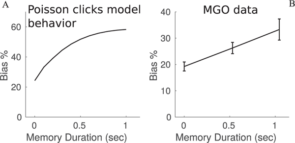
Postcategorization bias grows with memory period duration. (Left) Model prediction for bias during unilateral muscimol inactivation of the FOF as a function of increasing memory period duration. The model produces a bias that increases over time. Bias is relative to control behavior at each memory duration. The model was fit to the Poisson clicks task, not the MGO task. (Right) Unilateral FOF inactivation data from Erlich et al. (2011) shows a bias that grows with memory period duration for MGO trials. Trials were either nonmemory or had a memory period sampled from a distribution with mean 750 msec. Memory period is the time from the end of the stimulus to the go signal. Both trial types had an additional effective memory period between the go signal and the rat’s response. Memory trials were binned by their memory durations into shorter or longer than 750 msec. The solid line shows the average bias on ipsilateral trials at each of the three time bins. Bias in each time duration is relative to control performance on the same time duration. Nonmemory trials show some bias, while longer memory periods have stronger biases. Note that the vertical axis scale is different between plots.
A robust signature of this noise-corrupted memory is a bias that grows over time. To examine whether this second mechanism of bias is present in the FOF, we would like to examine bias as a function of memory period duration. In the evidence accumulation task, the effective memory period is short with little variability across trials. A separate task, memory-guided orienting (MGO), has a variable duration memory period (Erlich et al., 2011). Erlich et al. (2011) performed unilateral muscimol inactivations of the FOF during the MGO task. In this data set, rats entered a center nose poke and were presented with an auditory stimulus indicating either a left or right reward. The rats then waited for a go signal that indicated they could leave the center nose poke and make their decision. Some trials, called nonmemory trials, had no delay between the stimulus and the go signal. These trials were similar to the Poisson clicks trials. Other trials, called memory trials, had a variable-length delay period drawn from a gaussian distribution with a mean of 750 ms. We quantified the effect of unilateral FOF inactivation in this data set by binning memory trials into two bins, shorter or longer than the mean duration. Nonmemory trials were put in a third bin. We compared the ipsilateral bias of the muscimol data relative to the control data in each time bin. This analysis reveals that the bias increases with the duration of the memory period, consistent with our model’s prediction (see Figure 6B).
Our model predicts a bias that grows faster over time; however, our model was fit to Poisson clicks data, not MGO data. We present the model prediction only to demonstrate the qualitative behavior of the model. Further, our model was fit to trials with short, fixed-duration memory periods. This demonstrates that both mechanisms of memory biases are present in the MGO data. First, nonmemory trials are biased while being set or decoded. Second, memory trials show time-dependent degradation of the memory.
3. Discussion
Unilateral inactivations of the FOF during two different decision-making tasks produce an ipsilateral bias characterized by a vertical scaling of the psychometric curve. While the stimulus-independent nature of this bias suggested a poststimulus-categorization effect of the perturbation, the neural mechanisms underlying that, and the question of whether the FOF itself participated in the categorization or is driven by an already-categorical signal was left unaddressed. Exploring these questions with a mutual inhibition model, we found that the experimental effects, including the vertical scaling of the psychometric curve, could be reproduced by a mutual inhibition model when acting as a postcategorization memory unit but not when integrating evidence or being part of categorizing accumulated evidence into a choice. Our findings are consistent with analysis of spike trains from the FOF during two decision-making tasks, which show categorical encoding of decision choices (Erlich et al., 2011; Hanks et al., 2015). This model provides further evidence that inactivation of the FOF is perturbing a fully postcategorization memory by suggesting a neural mechanism for this bias.
The postcategorization model has two additional properties that are consistent with the data. First, both the model and the data show sensitivity to inactivation at the end of the stimulus period while being insensitive to inactivation at the start of the stimulus period. This temporal pattern of bias is a consequence of the postdecision memory function of the model and emerges without fitting directly to the optogenetic data. Second, the model makes a prediction that bias should grow with increasing memory perids. Post hoc examination of memory-guided orienting data demonstrated time-dependent increases in bias.
3.1. Biological Details.
This model opens a number of questions about how a simple memory model might be implemented in a cortical circuit. First, where does the transformation from a graded evidence signal into a categorized evidence signal take place? Our model fitting suggests that the bistable dynamics of the FOF are insufficient to compute the transformation without changing the type of bias. One barrier to examining this question is our limited knowledge of how the accumulated evidence is represented in the brain. It is also possible that a subset of cells in the FOF computes this transformation in a feedforward fashion. Spike trains recorded from the FOF show a wide distribution of tuning curves, meaning that some cells represented the accumulated evidence in a graded fashion.
Second, cell tuning in the FOF does not appear to be lateralized. Cells in the FOF show left and right orientation firing preferences with roughly equal percentages (Erlich et al., 2011; Hanks et al., 2015). How does a unilateral inactivation produce an ipsilateral bias given the lack of lateralization? One possibility is that there is lateralization in the FOF in the number of cells that project to subcortical structures. A recent study in mouse premotor cortex (ALM) found that cells are not lateralized by firing preference, but the cells that project subcortically are lateralized (Li, Chen, Guo, Gerfen, & Svoboda, 2015). Although ALM and FOF could have important functional differences, lateralization of subcortical projections is a possible mechanisms of bias. A recent study suggested that the FOF is part of a larger memory network including the superior colliculus (Kopec et al., 2015). If that is true, then blocking subcortical projections might disrupt the ipsilateral coding more than the contralateral coding.
Third, bilateral inactivations of the FOF during the Poisson clicks task were better described by a leaky integration process than a bidirectional lapse rate (Erlich et al., 2015). Our model produces a bidirectional lapse rate during bilateral inactivations. We did not directly model the temporal evolution of the evidence integration process in the postcategorization model, so the model cannot address the apparent leaky integration process. Erlich et al. (2015) hypothesized the existence of a parallel leaky integration circuit that becomes dominant when the FOF is bilaterally inactivated. Our model cannot speak directly to this hypothesis and could be consistent with either outcome. A further possibility is that some cells in the FOF are involved in the integration of evidence but are not lateralized, while the postcategorization memory circuit has lateralized projections subcortically. If this was true, then unilateral inactivations would bias the postcategorization memory but not the evidence integration process. Additionally, bilateral inactivations would perturb the evidence integration process, potentially producing a shorter integration time constant. This hypothesis predicts that bilateral optogenetic inactivations would perturb behavior during the first half of the evidence period, unlike our model.
3.2. Relationship to Other Modeling Studies.
Our modeling study has some similarities to and differences from other recent studies in the literature, and we conclude by providing a few comments. First, Wong and Wang (2006) propose a model in which evidence integration and decision memory happen in the same network. Our analysis suggests that this situation is not compatible with the FOF data; instead, we offer a picture of an integration process feeding into a short-term memory network. Our model executes the same computations as Wong and Wang (2006) model but separated in space. Spatial separation of evidence accumulation, decision thresholding, and decision memory mechanisms have been proposed in the human neuroscience literature (Simen, 2012) and have been used to described human EEG data (van Vugt, Simen, Nystrom, Holmes, & Cohen, 2014). Our study adds to this literature by examining which of these mechanisms can explain causal perturbation data to rodents.
Second, recent studies have examined unilateral and bilateral inactivations of a mouse prefrontal area known as ALM (Guo et al., 2014; Li, Daie, Svoboda, & Druckmann, 2016). One study found that behavioral performance and network activity recovered from unilateral inactivations, but not after bilateral inactivations (Li et al., 2016). Associated modeling proposed modular redundant networks that could recover from unilateral inactivation, examining both modular memory and modular integration networks. Here, we examined an orthogonal question. We examined full trial inactivations from which the network activity does not recover and asked what computations are consistent with the pattern of bias from the perturbed network.
3.3. Conclusion.
Simple models using neural-like elements can reproduce the temporal and stimulus-difficulty patterns of bias caused by unilateral inactivation of the FOF in two different behavioral tasks, but only when the computational role of the FOF is configured to be maintenance of post-categorization decision memory. These results extend and support the findings of (Erlich et al., 2015).
Acknowledgments
We thank members of the Brody lab for useful discussions. J. E. is supported by Program of Shanghai Academic/Technology Research Leader (15XD1503000) and by the Science and Technology Commission of Shanghai Municipality (15JC1400104). This work was supported by NIH grant 5R01MH08358.
Appendix
Appendix: Methods
A.1. Data Sets.
Our analysis examines several data sets. First are unilateral muscimol inactivations of the FOF during the Poisson clicks task as described in Erlich et al. (2015). This data set was used in Figures 1 and 3. Second, we used unilateral optogenetic inactivations of the FOF during the Poisson clicks task as described in Hanks et al. (2015). The trials in this data set were used in Figure 5 to simulate the model. The rat choices were not used. Third are the unilateral muscimol inactivations of the FOF during memory-guided orienting (MGO) task described in Erlich et al. (2011). This data set was used in Figure 6. A fourth data set, unilateral optogenetic inactivations of the FOF during the MGO task, was not analyzed here but was extensively and comparably analyzed in Kopec et al. (2015).
We used each of these data sets as presented in their original papers; we did not exclude any rats or sessions. For each of these data sets, we analyzed the meta-rat data set produced by combining inactivation sessions from all the rats together. In general, we also combined data sets from left-and right-side inactivations to produce a larger combined data set. This merging was done by switching the labels of left and right choices and stimuli. Confidence intervals were computed using the 95% CI from a binomial distribution.
A.2. Quantifying Post-Categorization Bias.
Postcategorization bias was measured as the percentage of “go left” (or “go right”) trials that flipped to a right choice (or left choice) out of the number of “go left” (or “go right”) trials in the control data set. In terms of right hemisphere inactivations,
| (A.1) |
B is the bias, M is the muscimol psychometric curve (expressed in a probability of going right), and C is the control psychometric curve. In terms of left hemisphere inactivations,
| (A.2) |
B is then a curve of the bias at each point along the click difference axis, which is the independent axis of the psychometric curve. Sometimes B is averaged across the click difference axis to get a single number bias.
A.3. Quantifying Bilateral Impairment.
For data and simulations with bilateral inactivations, the psychometric curve flattens, indicating impairment rather than producing a bias. We quantified this impairment by computing the postcategorization bias on each side of the psychometric curve. We used equation A.1 for impairment on the left half of the psychometric curve and equation A.2 for impairment on the right half of the psychometric curve. These two impairments were averaged into one impairment score reported in the text.
A.4. Model Fitting.
The mutual inhibition model used in our study was used previously in Kopec et al. (2015) and numerically simulated using the same approach as Kopec et al. (2015). Given that the model contains stochastic inputs, we cannot simply evaluate a single trajectory of the model because the response with the same parameters would be dependent on the specific realization of the stochastic noise. In order to get a reliable model response to the same parameters, one possibility would be to simulate many trials with different realizations of the noise. An alternative strategy, used in this study, was to compute the entire probability distribution of possible model responses given all noise realizations. (See section A.5 and Brunton et al., 2013, for a detailed description of this numerical algorithm.)
The integration model was implemented by numerically simulating every trial in the data set using the actual click trains as input to the model. The length of the memory period on each trial was the duration from when the center light went off, indicating to the rat the evidence period had ended, and when the rat left the center nose poke. For each trial, the model output was the probability of choosing left or right given the model parameters θ. By assuming independent trials, we can compute the likelihood of the data by the product of the probability of the rat’s choice on each trial:
| (A.3) |
| (A.4) |
We then used gradient descent to minimize the —LL. We found the model had local minima, so we used 100 restarts of gradient descent with random initial conditions. Parameter uncertainty was estimated by approximating the local likelihood landscape with a gaussian. The Hessian of the negative log-likelihood function was estimated using finite difference methods. The inverse of the Hessian is the standard estimator for the covariance of the parameter estimates (Daw, 2011). This means each diagonal entry is the variance of each parameter alone, and their square roots are the standard error of that parameter. Table 1 reports the standard error for each parameter.
The categorization and postcategorization models were not evaluated by simulating every trial. Given that integration dynamics from individual trials were captured by the term, we discretized a values and simulated the model response to each a value. Each simulation had an evidence period 1 s in duration, where the input from accumulation value was constant in time. The stimulus period was followed by a 100 msec memory period with no input. The model’s response probability for each trial was computed by multiplying the probability of accumulation values for that trial’s click difference, by the probability of model response for that accumulation value, . We then used the same likelihood function and gradient descent methods as the integration model.
The postcategorization model was also fit to the bilateral and unilateral inactivation data simultaneously. The likelihood function was modified so trials from three separate groups were weighted equally: control trials, unilateral inactivation trials, and bilateral inactivation trials. This weighting was done to prevent an unequal number of trials from distorting the model fit.
A.5. Numerical Simulation of the Mutual Inhibition Model.
Our model is a two-dimensional nonlinear stochastic differential equation. We used a numerical procedure to obtain the probability distribution over model responses. This procedure is a generalization of the Euler-Maruyama algorithm (also known as the stochastic Euler algorithm) from simulating a single sample trajectory to simulating the distribution over trajectories. Rather than track the dynamics of a single trajectory, we track the dynamics of probability mass. We provide a brief description of the Euler-Maruyama algorithm and our generalization of it. Consider a stochastic differential equation (SDE) of the form
| (A.5) |
which describes the time evolution of a variable with a time constant τ, deterministic dynamics G(x), and an additive white noise process W with variance σ2. This SDE may also be written as a Fokker-Planck equation, a partial differential equation that tracks the evolution of the probability density function of x:
| (A.6) |
The Fokker-Planck equation may be solved analytically or numerically simulated (Risken, 1989).
The Euler-Maruyama algorithm, like its deterministic version, starts from a first-order Taylor series expansion of the deterministic dynamics. On each time step, the state variable takes a step in the direction given by G(x), plus a random variable with variance scaled relative to the time step:
| (A.7) |
In order to track probability mass, we discretize our state space into spatial bins. Let fi,t be the probability mass in the ith spatial bin at time t. In the t + Δt time step, this mass will be displaced by deterministic motion given by Let be the coordinates of the center of the ith bin. Centered at the end point of this deterministic step we have gaussian dispersion with variance . The gaussian dispersion represents the distribution of possible noise realizations for this time step. Let n be a grid over this gaussian, with grid spacing much smaller than the grid over state space. The probability mass in each noise bin n is settled into state-space bins such that the mean location of the mass is at , the state-space coordinate of ni. This preserves the mean of the probability distribution. In practice, for a given set of parameters, this algorithm can be written into a set of Markov transition matrices F, so each time step iteration is given by
| (A.8) |
where the F used is dependent on the current inputs into the model.
The supplementary materials of Brunton et al. (2013) offer more description of this numerical algorithm. The major bottleneck is the computation of the F matrices. Once it has been computed, the algorithm has (m3t) time complexity where m is the number of spatial bins and t is the number of timesteps.
A.6. Model Validation and MetaParameter Choices.
To ensure the numerical simulation was working correctly, model behavior was compared to an ensemble of sample trajectories from the Euler-Maruyama method. This allowed verification that the mean and variance of the distribution were correct. In addition, the fixed points of the deterministic system were computed analytically for an example parameter set and agreed with the numerical results. Several metaparameters needed to be determined for use in all simulations: the spatial boundaries, the number of spatial bins, and the time step size. We performed the numerical simulation over the internal variable state space (−4, 4). Beyond this domain, the external variable changes very little. We found that 40 spatial bins in each dimension (for a total of 1600 bins) and a time step of 10 msec had high accuracy and reasonable computational cost. In contrast to most numerical methods, increasing the time step may not lead to more accurate results unless the spatial bins scale as well. Given that the spatial bins are the larger computational bottleneck, the time step was selected based on the spatial bins.
A.7. Computing P(a|ΔR,L).
An evidence accumulation model as described in Brunton et al. (2013) was fit to the control behavior sessions. Each trial in the data set was simulated using this accumulation model to get the distribution of accumulation values at the end of the trial P(a|tend). This distribution was averaged over all trials with the same click difference to get P(a|ΔR,L). The model was evaluated with different bin sizes for the click difference and accumulator values. The results did not depend on these choices.
A.8. Cross-Validation.
In order to assess how well different model architectures generalized beyond the data used to fit the model, we used two-fold cross-validation. The data were split into two equal data sets with the same number of trials from each individual rat going into each set. For each set, the data were fit to one half with 100 random initial parameter restarts of gradient descent. The parameters that best fit the training half were then tested on the other half. The likelihoods on the two test sets were averaged to produce the total likelihood.
A.9. Constructing a Psychometric Curve from the Model Output.
Once the model has been fit, to construct a psychometric curve P(a|ΔR,L) we multiply the vector of model go-right probabilities given accumulator values, P(R|a), with the matrix of P(a|ΔR,L)accumulator value probabilities given click differences.
A.10. Simulating Temporally Precise Inactivations.
During the temporally precise inactivation simulations, we wanted to simulate the trajectories of the evidence accumulation variable “a.” We simulated sample trajectories of both the evidence accumulation model used to construct P(a|ΔR,L) and the mutual inhibition model. We simulated 14,000 trials from the opto-genetic data set in Hanks et al. (2015). For each trial, we computed 100 sample trajectories. From these 140,000 trials, we computed the bias during each of the inactivation patterns (see Figure 5). In order to accurately estimate the uncertainty of our model, we performed a boostrapping procedure. We generated 100 bootstrapped data sets where we pulled one of the 100 sample trajectories from each trial and computed the bias on this bootstrapped data set. This preserved the distribution of different trial types across the 14,000 trials but sampled the variability of model responses across the 100 sample trajectories.
A.11. Tuning Curve.
A tuning curve for the FOF model was constructed following the method developed in Hanks et al. (2015). First, a collection of trials was generated. Then, for each trial, a sample trajectory of the accumulation variable was used as input to the postcategorization model producing the firing rate for the model and a behavioral choice. The trial and the behavioral choice were used to produce the distribution of accumulation values from the evidence accumulation model from (Brunton et al., 2013). Consistent with Hanks et al. (2015), we used the backward propagation model, which utilizes the behavioral choice to produce a more accurate model of the accumulation variable.
A.12. Memory-Guided Orienting Data.
To evaluate how postcategorization bias increases with the memory period duration, we binned trials by their stimulus difficulty and the duration of the memory period. The memory period was defined as the duration between the end of the stimulus and the go signal. All trials had an additional effective memory period between the go signal and the rat’s response. However, this duration did not depend on the length of the memory period, so we did not use it in our analysis. The markers shown in Figure 5 are placed at the center of each bin in time (on the x-axis).
Footnotes
There are no competing interests.
Contributor Information
Alex T. Piet, Princeton Neuroscience Institute, Princeton University, Princeton, NJ 08544, U.S.A.
Jeffrey C. Erlich, NYU-ECNU Institute of Brain and Cognitive Science, New York University Shanghai, Shanghai 200122, China
Charles D. Kopec, Princeton Neuroscience Institute and Department of Molecular Biology, Princeton University, Princeton, NJ 08544, U.S.A.
Carlos D. Brody, Princeton Neuroscience Institute, Department of Molecular Biology, and Howard Hughes Medical Institute, Princeton University, Princeton, NJ 08544, U.S.A.
References
- Aljadeff J, Renfrew D, Vegué M, & Sharpee TO (2016). Low-dimensional dynamics of structured random networks. Phys. Rev. E, 93, 022302. [DOI] [PMC free article] [PubMed] [Google Scholar]
- Bogacz R, Brown E, Moehlis J, Holmes P, & Cohen JD (2006). The physics of optimal decision making: A formal analysis of models of performance in two-alternative forced-choice tasks. Psychological Review, 113(4), 700–765. [DOI] [PubMed] [Google Scholar]
- Brown KS, & Sethna JP (2003). Statistical mechanical approaches to models with many poorly known parameters. Phys. Rev. E, 68, 021904. [DOI] [PubMed] [Google Scholar]
- Brunton BW, Botvinick MM, & Brody CD (2013). Rats and humans can optimally accumulate evidence for decision-making. Science, 340(6128), 95–98. [DOI] [PubMed] [Google Scholar]
- Daw N (2011). Trial-by-trial data analysis using computational models. New York: Oxford University Press. [Google Scholar]
- Erlich J, Bialek M, & Brody C (2011). A cortical substrate for memory-guided orienting in the rat. Neuron, 72(2), 330–343. [DOI] [PMC free article] [PubMed] [Google Scholar]
- Erlich JC, Brunton BW, Duan CA, Hanks TD, & Brody CD (2015). Distinct effects of prefrontal and parietal cortex inactivations on an accumulation of evidence task in the rat. eLife, 4, e05457. [DOI] [PMC free article] [PubMed] [Google Scholar]
- Gradinaru V, Zhang F, Ramakrishnan C, Mattis J, Prakash R, Diester I, Deisseroth K (2010). Molecular and cellular approaches for diversifying and extending optogenetics. Cell, 141(1), 154–165. [DOI] [PMC free article] [PubMed] [Google Scholar]
- Guo Z, Li N, Ophir E, Gutnisky D, Ting J, Feng G, & Svoboda K (2014). Flow of cortical activity underlying a tactile decision in mice. Neuron, 81(1), 179–194. [DOI] [PMC free article] [PubMed] [Google Scholar]
- Hanks TD, Ditterich J, & Shadlen MN (2006). Microstimulation of macaque area lip affects decision-making in a motion discrimination task. Nat. Neurosci, 9(5), 682–689. [DOI] [PMC free article] [PubMed] [Google Scholar]
- Hanks TD, Kopec CD, Brunton BW, Duan CA, Erlich JC, & Brody CD (2015). Distinct relationships of parietal and prefrontal cortices to evidence accumulation. Nature, 520(7546), 220–223. [DOI] [PMC free article] [PubMed] [Google Scholar]
- Kopec C, Erlich J, Brunton B, Deisseroth K, & Brody C (2015). Cortical and subcortical contributions to short-term memory for orienting movements. Neuron, 88(2), 367–377. [DOI] [PMC free article] [PubMed] [Google Scholar]
- Li N, Chen T-W, Guo ZV, Gerfen CR, & Svoboda K (2015). A motor cortex circuit for motor planning and movement. Nature, 519(7541), 51–56. [DOI] [PubMed] [Google Scholar]
- Li N, Daie K, Svoboda K, & Druckmann S (2016). Robust neuronal dynamics in premotor cortex during motor planning. Nature, 532(7600), 459–464. [DOI] [PMC free article] [PubMed] [Google Scholar]
- Machens CK, Romo R, & Brody CD (2005). Flexible control of mutual inhibition: A neural model of two-interval discrimination. Science, 307(5712), 1121–1124. [DOI] [PubMed] [Google Scholar]
- Mante V, Sussillo D, Shenoy KV, & Newsome WT (2013). Context-dependent computation by recurrent dynamics in prefrontal cortex. Nature, 503(7474), 78–84. [DOI] [PMC free article] [PubMed] [Google Scholar]
- Risken H (1989). The Fokker-Planck equation: Methods of solution and applications (2nd ed.). New York: Springer. [Google Scholar]
- Scott BB, Constantinople CM, Erlich JC, Tank DW, & Brody CD (2015). Sources of noise during accumulation of evidence in unrestrained and voluntarily head-restrained rats. eLife, 4, e11308. [DOI] [PMC free article] [PubMed] [Google Scholar]
- Simen P (2012). Evidence accumulator or decision threshold: Which cortical mechanism are we observing? Frontiers in Psychology, 3,183. [DOI] [PMC free article] [PubMed] [Google Scholar]
- Sussillo D, & Barak O (2012). Opening the black box: Low-dimensional dynamics in high-dimensional recurrent neural networks. Neural Computation, 25(3), 626–649. [DOI] [PubMed] [Google Scholar]
- van Vugt MK, Simen P, Nystrom L, Holmes P, & Cohen JD (2014). Lateralized readiness potentials reveal properties of a neural mechanism for implementing a decision threshold. PloS One, 9(3), 1–13. [DOI] [PMC free article] [PubMed] [Google Scholar]
- Wichmann FA, & Hill NJ (2001). The psychometric function: I. Fitting, sampling, and goodness of fit. Perception and Psychophysics, 63(8), 1293–1313. [DOI] [PubMed] [Google Scholar]
- Wong K-F, & Wang X-J (2006). A recurrent network mechanism of time integration in perceptual decisions. Journal of Neuroscience, 26(4), 1314–1328. [DOI] [PMC free article] [PubMed] [Google Scholar]
- Yoon K, Buice MA, Barry C, Hayman R, Burgess N, & Fiete IR (2013). Specific evidence of low-dimensional continuous attractor dynamics in grid cells. Nat. Neurosci, 16(8), 1077–1084. [DOI] [PMC free article] [PubMed] [Google Scholar]