Consistent Spatial-Temporal Longitudinal Atlas Construction for Developing Infant Brains

Abstract

Brain atlases are an essential component in understanding the dynamic cerebral development, especially for the early postnatal period. However, longitudinal atlases are rare for infants, and the existing ones are generally limited by their fuzzy appearance. Moreover, since longitudinal atlas construction is typically performed independently over time, the constructed atlases often fail to preserve temporal consistency. This problem is further aggravated for infant images since they typically have low spatial resolution and insufficient tissue contrast. In this paper, we propose a novel framework for consistent spatial-temporal construction of longitudinal atlases for developing infant brain MR images. Specifically, for preserving structural details, the atlas construction is performed in spatial-temporal wavelet domain simultaneously. This is achieved by a patch-based combination of results from each frequency subband. Compared with the existing infant longitudinal atlases, our experimental results indicate that our approach is able to produce longitudinal atlases with richer structural details and also better longitudinal consistency, thus leading to higher performance when used for spatial normalization of a group of infant brain images.

I. INTRODUCTION

DURING the early postnatal period, the human brain undergoes dramatic changes in size, shape, structures and functions. For example, volumetric studies based on MR images have shown that the total brain volume increases 101% in the first year, followed by an additional 15% in the second year [1]. Therefore, longitudinal study is important to understand mechanisms of both normative and pathological developments in infant brains. Although several state-of-the-art infant longitudinal atlases have been developed [2]–[7], most of them were built independently over time, thus leading to temporal inconsistency.

The goal of longitudinal atlas construction is to estimate a sequence of atlases that capture the trend of anatomical changes in a population of images [8], [9]. Davis et al. [10] constructed a serial of atlases over a time interval from 18 through 96 years of age using a diffeomorphic growth model and Nadaraya-Watson kernel regression. Dittrich et al. [11] constructed a spatio-temporal latent atlas for capturing fetal brain evolution covering the period of 20–30 gestational weeks. This study provided a developing template that serves as a standard for estimating the age of fetus based on the brain structures.

In pediatric, neonatal, and fetal research, specific longitudinal atlases are needed. But the dynamic development of brain structures present large challenges in consistently estimating a sequence of atlases. Shi et al. [2] proposed infant atlases using unbiased group-wise registration, involving 95 normal infants (56 males and 39 females) with MR images scanned at 3 time points, i.e., neonate, 1-year-old and 2-years-old. Kuklisova-Murgasova et al. [3] constructed atlases for preterm babies aged from 29 to 44 weeks using affine registration. Oishi et al. [12] proposed to combine affine and non-linear registrations for hierarchically building an infant brain atlas. Their atlas was built from babies of 37–53 post-conceptional weeks. Fonov et al. [4] applied a non-linear unbiased registration framework on the NIH pediatric database and ICBM atlas data, and then created unbiased atlas sequences for age ranges 0–4.5 years old and 4.5–18.5 years old, respectively. On the other hand, by using adaptive kernel regression and group-wise registration, Serag et al. [5] constructed a spatiotemporal brain atlas of the preterm babies aged from 29 to 44 weeks. Habas et al. [6] proposed a spatiotemporal atlas of the fetal brain with gestational ages ranging from 20.57 to 24.71 weeks. Group-wise registration and voxel-wise nonlinear modeling were applied to capture the appearance of brain structures over time.

The creation of an atlas requires the mapping of a population into a common space. Constructing longitudinal atlases is even more complicated due to anatomical variations caused by brain development. So far, longitudinal atlas construction methods can be broadly classified into two categories: (1) Kernel regression or mixture modeling over the time domain [3], [5], [10], [13]: (2) Jointly aligning subject image sequences to a template sequence [14]–[16]. In the first category of kernel regression based methods, longitudinal atlases at different time points are constructed by a kernel regression over time. For example, Gholipour et al. [13] integrated spatial symmetric normalization with temporal kernel regression for atlas sequence construction. Fishbaugh et al. [8] proposed to estimate the dynamics of brain tumor shape change through a period of 12 months using geodesic shape regression model. However, all these approaches neglected the important subject-specific longitudinal information, leading to temporal inconsistency. In the second category of joint registration methods [14], [15], subject-specific evolutions are first explicitly estimated using regression models. Then, spatial-temporal pairwise registration is performed between each subject’s image sequence and the atlas sequence. Finally, an atlas sequence can be constructed after aligning all subjects to the template space. Such methods assume a consistent common space for the longitudinal data, and thus propose to estimate the atlas sequence by jointly optimizing the atlas space and the atlas evolution model. For instance, Liao et al. [15] constructed longitudinal atlas for Alzheimer’s disease patients. This work efficiently incorporated both the subject-specific information and population information by iteratively updating both the atlas growth model and the atlas sequence using group-wise registration.

More recently, patch-based sparse representation has been proposed for detail-preserving atlas construction [17]–[19]. In [17], [19], consistent brain structures that occur in the local neighborhood were used to refine atlas construction. This method has been further extended to the frequency domain [18], [20], [21] to improve the preservation of anatomical details.

In this paper, we propose a novel framework for consistent temporal construction of longitudinal atlases for developing infant brain MR images in the first year of life. Here, temporal consistency means brain structural consistency in the temporal/longitudinal domain. For example, if a small cortical structure appears in both month 1 and month 12, we can expect it appearing also in month 6. By introducing this temporal consistency term, we can explicitly impose each structure to be consistent across different time-points. Specifically, atlas construction can be conducted in the spatial-temporal wavelet domain simultaneously. First, each brain image is decomposed into frequency subbands using wavelet transform for improving detail preservation. Then, the atlas is constructed on each frequency subband using a patch-based mechanism. Furthermore, for each image patch, we fuse both temporally-related variability and spatial local variability by group-sparse construction. In addition, we supervise the construction process by anatomical priors in the form of tissue probability maps. Finally, we apply our method to construct longitudinal brain atlases from infant MR images, which often suffer from low spatial resolution and insufficient tissue contrast. Experimental results indicate that our approach is able to produce longitudinal atlases with richer structural details and better longitudinal consistency, thus enabling achieving higher performance when applied to spatial normalization of a group of infant brain images. Pipeline of the whole paper is presented in Fig. 1. Table T1 in the supplementary materials (available in the supplementary files /multimedia tab) summarizes the important notations and their corresponding definitions throughout this paper.

Fig. 1.

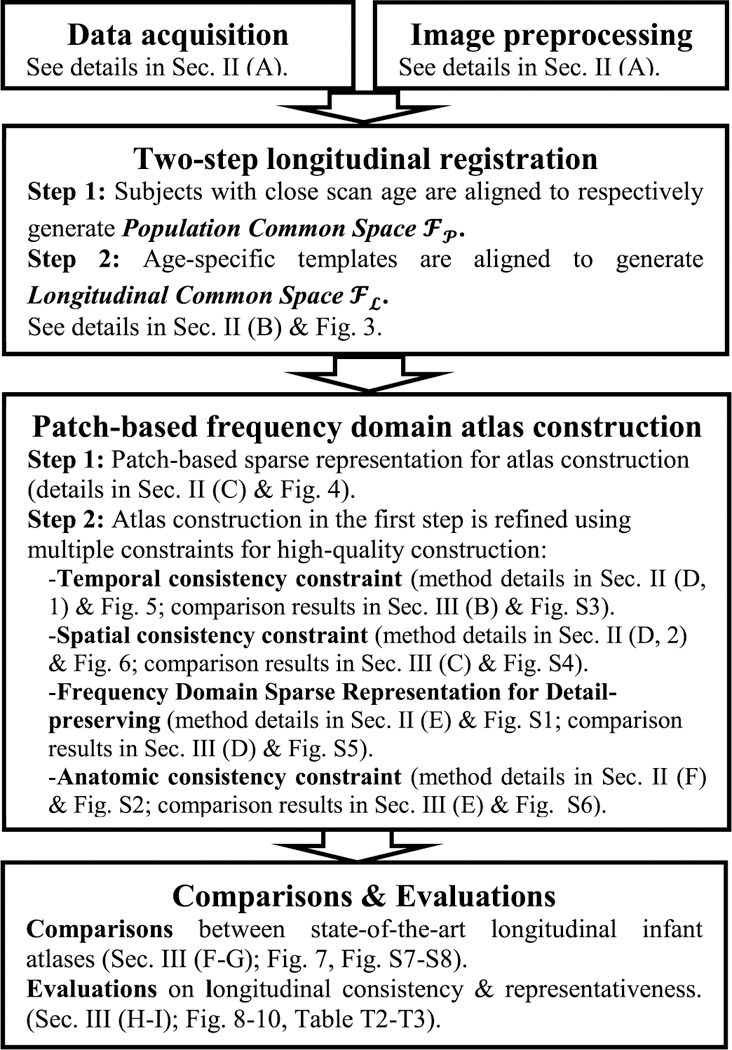
Flow chart of the proposed method; Figs. S1–S8 in supplementary materials are available in the supplementary files /multimedia tab.

II. METHOD

A. Data Acquisition and Image Preprocessing

Serial T1-weighted and T2-weighted MR images of 35 healthy infants (18 males/17 females) were acquired using a Siemens 3T head-only MR scanner with a 32 channel head coil. Each infant was scheduled to be scanned every 3 months in the first year since birth. Due to insufficient quality and uncompleted scans, each infant has different number of scans, ranging from 2 to 5 in the first year. In total, 150 high-quality MR scans from 35 infants were acquired, with each infant having 4.3 scans on average, and the number of subjects at each scan time is shown in Fig. 2.

Fig. 2.

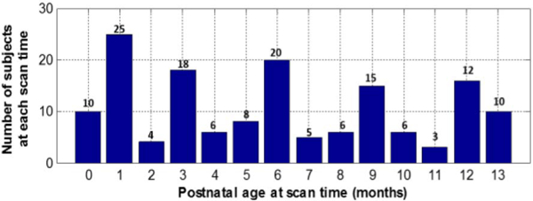
Number of subjects at each postnatal age at time of scan.

For these subjects, T1-weighted MR images (144 sagittal slices) were acquired with the imaging parameters:

TR/TE = 1900/4.38 ms, flip angle = 7°, and resolution = 1 × 1 × 1mm³. T2-weighted MR images (70 axial slices) were acquired with the parameters: TR/TE = 7380/119 ms, flip angle = 150°, and resolution = 1.25 × 1.25 × 1.95 mm³.

All images were preprocessed with a standard pipeline in iBEAT software [37]. Briefly, it includes the following major steps: 1) rigid alignment of T2 image onto its T1 image and further resampling to be of 1 × 1 × 1 mm³ using FLIRT in FSL [22]; 2) skull stripping by a learning-based method [23] and further removal of cerebellum and brain stem by registration with an atlas [24]; 3) correction of intensity inhomogeneity by N3 [25]; 4) longitudinally-consistent tissue segmentation by an infant-dedicated, 4D level-set method [26].

B. Image Normalization by Longitudinal Group-Wise Registration

A two-step registration strategy is implemented as shown in Fig. 3. In the first step of age-specific population registration (Fig. 3(a)), we use kernel-based regression to produce a series of local age-dependent anatomical templates and tissue probability maps. Specifically, the source images of different subjects at neighboring ages are first aligned using a publicly available group-wise non-linear registration method [27] to form an age-specific Population Common Space ${\mathcal{F}}_{\mathcal{P}}$. Given a set of N source images $\left\{I_n\left(t^m\right)\in {ℝ}^3|n=1,\cdots ,N\right\}$ around a time point t^m (m = 1, ∙ ∙ ∙, M), where M denotes the number of longitudinal atlases used to represent the time range, the population common space is produced using transformations {A_n(t^m)|n = 1, ∙ ∙ ∙, N}. To create the age-dependent average template, we use kernel regression and also use {t₁, ∙ ∙ ∙, t_N} to denote the postnatal age of each subject at the time of scan. The average anatomy $\overline{I}\left(t^m\right)$ is then calculated by:

$$\overline{I}\left(t^m\right)=\frac{{\sum }_{n=1}^N\omega \left(t_n,t^m\right)·I_n{\left(t^m\right)}^{°}{A}_n\left(t^m\right)}{{\sum }_{n=1}^N\omega \left(t_n,t^m\right)}$$ (1)

Fig. 3.

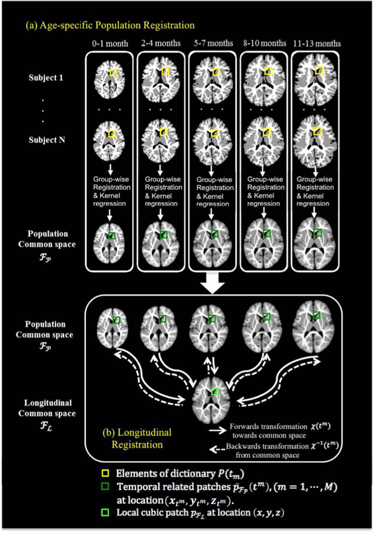
Flow chart of the two-step longitudinal image registration framework. (a) Age-specific population registration to produce Population Common Space F_P; (b) Longitudinal registration to produce Longitudinal Common Space F_L.

Where we use a Gaussian kernel to calculate the weight:

$$\omega \left(t_n,t^m\right)=\frac{1}{\sigma \sqrt{2\mathit{\pi }}}\exp \left(-\frac{{\left(t_n-t^m\right)}^2}{2{\sigma }^2}\right)$$ (2)

In the second step, a longitudinal registration is performed (Fig. 3(b)). The age-specific templates $\left\{\overline{I}\left(t^1\right),\cdots ,\overline{I}\left(t^M\right)\right\}$ are aligned using the GLIRT group-wise non-linear registration method [27]. A set of transformations {χ(t¹), ∙ ∙ ∙ ,χ(t^M)} connects the age-specific templates to generate the Longitudinal Common Space ${\mathcal{F}}_{\mathcal{L}}$. When we consider a local cubic patch ${\overline{p}}_{{\mathcal{F}}_{\mathcal{P}}}\left(t^m\right)$ centered at location (x_tm, y_tm, z_tm) in the average anatomy $\overline{I}\left(t^m\right)$ of the m- th time point (e.g., one of the dark green cube in Fig.3 (b)), its temporally-related patch ${\overline{p}}_{{\mathcal{F}}_{\mathcal{P}}}\left(t^{m^{\prime }}\right)$ can be located using the transformation set {χ(t¹), ∙ ∙ ∙ ,χ(t^M)} through Longitudinal Common Space ${\mathcal{F}}_{\mathcal{L}}$ as: ${\overline{p}}_{{\mathcal{F}}_{\mathcal{P}}}\left(t^{m^{\prime }}\right)={\overline{p}}_{{\mathcal{F}}_{\mathcal{P}}}{\left(t^m\right)}^{°}\chi {\left(t^m\right)}^{°}{\chi }^{-1}\left(t^{m^{\prime }}\right)$. This process is shown in Fig. 3(b), where each dark green cube follows the solid arrow to the light green cube in the common space, and then searches for its temporally-related patch at another time point by tracing the dashed arrows.

C. Patch-Based Atlas Construction

Our atlas construction is performed in a patch-by-patch manner. We consider a local cubic patch $p{\mathcal{F}}_{\mathcal{L}}$ centered at location (x, y, z) in the Longitudinal Common Space ${\mathcal{F}}_{\mathcal{L}}$. As shown in Fig. 3, following the reversed transformations {χ^–1(t¹), ... ,χ^–1 (t^M)}, a number of M temporally-related patches $\left\{{\overline{p}}_{{\mathcal{F}}_{\mathcal{P}}}\left(t^1\right),\cdots ,{\overline{p}}_{{\mathcal{F}}_{\mathcal{P}}}\left(t^M\right)\right\}$ centered at locations $\left\{\left(x_{t}1,y_{t}1,z_{t^1}\right),\dots ,\left(x_{t}M,y_{t}M,z_{t}M\right)\right\}$ in each of the age-specific templates $\left\{I\left(t^1\right),\cdots ,I\left(t^M\right)\right\}$ are extracted. The patches are computed by:

$${\overline{p}}_{{\mathcal{F}}_{\mathcal{P}}}\left(t^m\right)=p_{{\mathcal{F}}_{\mathcal{L}}}°{\chi }^{-1}\left(t^m\right)$$ (3)

All these patches are represented as a vector of length V_tm = v_tm × v_tm × v_tm, where v_tm is the patch size in each dimension at each time point. We sparsely refine each of the M patches ${\overline{p}}_{{\mathcal{F}}_{\mathcal{P}}}\left(t^m\right)$, (m = 1, ∙ ∙ ∙, M), using a dictionary that is formed by including all patches at the same location in all N training images enclosed at time t^m as shown in Fig. 4, i.e., $P\left(t^m\right)=\left[p_1\left(t^m\right),p_2\left(t^m\right),\cdots ,p_N\left(t^m\right)\right],(m=1,\cdots ,M)$, (m = 1,..., M), thereby generating a constructed atlas patch p^atlas(t^m). To compensate for possible registration error, we enrich the dictionary by including patches from neighboring locations, i.e., 26 locations immediately adjacent to (x_tm, y_tm, z_tm). Therefore, from all N aligned images, we will have a total of $N_{\mathit{\text{total}}}^{t^m}=27\times N$ patches in the dictionary, i.e., $P\left(t^m\right)=\left[p_1\left(t^m\right),p_2\left(t^m\right),\cdots ,p_{N_{total}^m}\left(t^m\right)\right]$. We use this dictionary to construct the refined atlas patch p^atlas(t^m) by estimating a sparse coefficient vector $\widehat{\beta }\left(t^m\right)$, with each element denoting the weight of the contribution of a patch in the dictionary. The construction problem can now be formulated as:

$$\widehat{\beta }\left(t^m\right)=\underset{{\hat{\beta }}^{t^m}>0}{\text{argmin}}{\Vert {\overline{p}}_{{\mathcal{F}}_{\mathcal{P}}}\left(t^m\right)-P\left(t^m\right)·\widehat{\beta }\left(t^m\right)\Vert }_2^2+\lambda {\Vert \widehat{\beta }\left(t^m\right)\Vert }_1$$ (4)

Fig. 4.

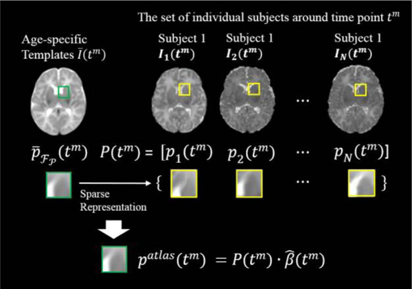
Demonstration of the patch-based atlas construction, using the 1-month time-point images as an example.

where λ is a non-negative parameter controlling the influence of the regularization term. Here, the first term measures the discrepancy between observations ${\overline{p}}_{{\mathcal{F}}_{\mathcal{P}}}\left(t^m\right)$ and the constructed atlas patch $p^{atlas}\left(t^m\right)=P\left(t^m\right)·\widehat{\beta }\left(t^m\right)$, and the second term is for L₁-regularization on the coefficients in $\widehat{\beta }\left(t^m\right)$.

D. Spatial-Temporal Consistency Constraint

To promote local consistency, we use multi-task LASSO [28] for spatial and temporal regularization in the space-time domain by solving for G × M neighboring atlas patches, indexed as g = 1, ..., G for the spatial neighboring patches and m = 1, ..., M for the temporal neighboring patches, simultaneously.

1). Temporal Consistency:

As illustrated in Fig. 5(a), we extract M temporally-related patches ${\overline{p}}_{{\mathcal{F}}_{\mathcal{P}}}\left(t^m\right)$, $(m=1,\cdots ,M)$ from each of the M age-specific population-average templates $\left\{\overline{I}\left(t^1\right),\cdots ,\overline{I}\left(t^M\right)\right\}$. We denote the age-dependent dictionary, training patch, and sparse coefficient vector for the m-th time-point as $P\left(t^m\right)$, ${\overline{p}}_{{\mathcal{F}}_{\mathcal{P}}}\left(t^m\right)$ and $\beta \left(t^m\right)$ respectively. We let $B^{Time}=\left[\beta \left(t^1\right),\cdots ,\beta \left(t^M\right)\right]$, which can also be written in the form of row vectors: B^Space $B^{Time}=\left[\begin{array}{c}{\gamma }_1^{Time}\\ ⋮\\ {\gamma }^{Time}\\ N_{total}^{t^m}\end{array}\right]$, where ${\gamma }_d^{Time}$ is the d- th row in the matrix $B^{Time}$, the number $N_{\mathit{\text{total}}}^{t^m}$ denotes the number of elements in dictionary P (t^m), and it is equal to the number of patch contained in the dictionary. Then, we reformulate

Fig. 5.

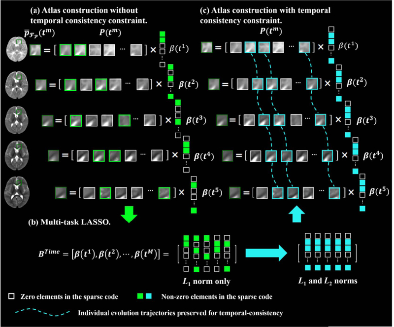
Comparison between the representations of temporally-related patches without/with temporal consistency constraint. (a) Without constraint, temporallyrelated patches are represented independently; (b) Multi-task LASSO is performed as Eq. (5), by optimizing both L₁ and L₂ norms, thus temporally-related patches share similar sparse coefficients. (c) With temporal consistency constraint, where temporally-related patches in the proposed atlases are generated using the same subject-specific evolution information. The temporal consistency of proposed longitudinal atlases is preserved.

Eq. (4) by using multi-task LASSO:

$$\begin{gathered} {\widehat{B}}^{Time}=\underset{{\widehat{B}}^{Time}}{\text{argmin}}\sum _{m=1}^M{\Vert {\overline{p}}_{{\mathcal{F}}_{\mathcal{P}}}\left(t^m\right)-P\left(t^m\right)·\beta \left(t^m\right)\Vert }_2^2 \\ +{\lambda }_T{\Vert {\widehat{B}}^{Time}\Vert }_{2,1} \end{gathered}$$ (5)

where ${\Vert {\widehat{B}}^{Time}\Vert }_{2,1}={\sum }_{d=1}^{N_{total}^{t^m}}{\Vert {\gamma }_d^{Time}\Vert }_2$. As shown in Fig. 5(b), the first term is a multi-task sum-of-squares term for all M temporally-related atlas patches. The second term is for multitask regularization using a combination of L₂ and L₁ norms. Here, L₂ norm penalization is imposed on each row of matrix ${\widehat{B}}^{Time}$ (i.e., ${\gamma }_d^{Time}$) to enforce the similarity of the temporally- related patches. L₁ norm penalization is imposed to ensure representation sparsity. This combined penalization ensures that the related patches have similar sparse coefficients. As illustrated in Fig. 5(c), this formulation facilitates all M patches to be generated using same subject-specific evolution information, in order to induce temporal consistency.

2). Spatial Consistency:

As demonstrated in Fig. 6 (a), we consider G spatial neighbors for patch $p_{{\mathcal{F}}_{\mathcal{L}}}$ centered at location (x, y, z) in the Longitudinal Common Space ${\mathcal{F}}_{\mathcal{L}}$ We denote the dictionary, training patch, and sparse coefficient vector for the g-th neighbor as P_g, p_g and β_g, respectively. For simplicity, we let B^Space = [β_1; ∙ ∙ ∙ ,β_G],which can also be written in the form of row vectors: $\left[\begin{array}{c}{\gamma }_1^{\mathit{Space}}\\ ⋮\\ {\gamma }_{N_{\mathit{\text{total}}}}^{\mathit{Space}}\end{array}\right]$ where ${\gamma }_d^{\mathit{Space}}$ is the d- th row in the matrix B^Space. Then, we reformulate (Eq. 4) using multi-task LASSO:

$${\widehat{B}}^{\mathit{Space}}=\underset{{\widehat{B}}^{\mathrm{Space}}>0}{\text{argmin}}\sum _{g=1}^G{\Vert p_g-P_g·{\beta }_g\Vert }_2^2+{\lambda }_S{\Vert B^{\mathit{Space}}\Vert }_{2,1}$$ (6)

Fig. 6.

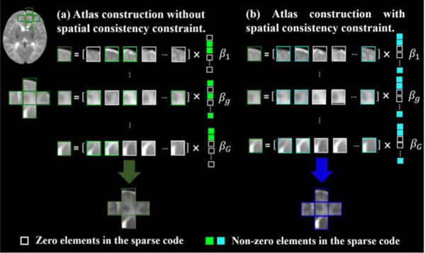
Comparison between the representations of spatially-neighboring patches without/with spatial consistency constraint. (a) Without constraint, where patches are represented independently; (b) Using spatial consistency constraint, neighboring patches are generated using the same subject-specific space information. Thus, the spatial consistency of proposed atlases is preserved.

3). Combination of Spatial and Temporal Consistency:

As discussed in Sections II D, spatial and temporal consistency of the longitudinal atlas sequence is achieved using two independent multi-task LASSO constraints. To achieve spatial- temporal consistency simultaneously, we need coupling these two constraints. We consider the G spatial neighbors for each of the M temporally-related patches. Thus, we can denote patch ${\overline{p}}_g\left(t^m\right)$ as the g-th spatial neighboring patch around patch $\overline{p}{\mathcal{F}}_{\mathcal{P}}\left(t^m\right)$ extracted from the template $\overline{I}\left(t^m\right)$, its dictionary as P_g (t^m), and sparse estimation as β_g (t^m). For constructing a number of G × M patches relatively, we construct the matrix ${\widehat{B}}^{S-T}=\left[{\beta }_1\left(t^m\right),\cdots ,{\beta }_G\left(t^m\right)\right]$ to fuse matrix B^Space and B^Time. Thus, Eq. (5) and Eq. (6) can be merged to Eq. (7):

$$\begin{gathered} {\widehat{B}}^{S-T}=\underset{{\widehat{B}}^{S-T}>0}{\text{argmin}}\sum _{g=1}^G\sum _{m=1}^M{\Vert {\overline{p}}_g\left(t^m\right)-P_g\left(t^m\right)·{\beta }_g\left(t^m\right)\Vert }_2^2 \\ +\lambda {\Vert {\widehat{B}}^{S-T}\Vert }_{2,1} \end{gathered}$$ (7)

where ${\Vert B^{S-T}\Vert }_{2,1}={\sum }_{d=1}^{N_{\mathit{\text{total}}}}{\Vert {\gamma }_d^{S-T}\Vert }_2$ The first term is the multi-task sum-of-squares term for all G × M patches. The second term is for multi-task regularization using the combination of L₂ and L₁ norms. L₂ norm penalization is imposed on each row of matrix $B^{S-T}\left(i.e.,{\gamma }_d^{S-T}\right)$, thus promoting the similarity of spatial neighboring and temporally-related patches simultaneously. The multi-task LASSO in Eq. (7) can be solved efficiently by using the algorithm described in [28].

E. Frequency Domain Sparse Representation for Detail-Preserving

As is shown in [29], image reconstruction in frequency domain is efficient for detail-preserving in single time-point atlas construction. Similarly, we perform atlas construction in the frequency domain given by wavelet transform. The proposed sparse patch-based atlas construction is performed in all frequency subbands, and the results are combined to give a final atlas sequence.

We first perform pyramidal decomposition using 3D wavelet on all images:

$$I=\sum _{f=1}^F{I}^{(f)}=\sum _{f=1}^F{D}^{(f)}·a^{(f)}$$ (8)

where f = 1, ∙ ∙ ∙, F denotes that the image I is decomposed into F frequency subbands. D^(f) denotes the wavelet basis of subband f, and a^(f) denotes the wavelet coefficients in subband f.

For our longitudinal atlas construction, the image components in subband f of the age-specific templates are denoted as: $\left\{{\overline{I}}^{(f)}\left(t^1\right),\cdots ,{\overline{I}}^{(f)}\left(t^M\right)\right\}$. We can locate the M temporally-related patches ${\overline{p}}_{{\mathcal{F}}_{\mathcal{P}}}^{(f)}\left(t^m\right),m=1,\cdots ,M$, centered at location (x_tm, y_tm, z_tm), and their spatial neighboring patches $p_g^{(f)}\left(t^m\right)$ in each subband f. Similarly, in the f -th subband component of all N training images, at the m-th time point, we include all patches at location (x_tm, y_tm, z_tm) and all its neighboring patches to build the dictionary, i.e., $P_g^{(f)}\left(t^m\right)=\left[p_1^{(f)}\left(t^m\right),p_2^{(f)}\left(t^m\right),\cdots ,p_N^{(f)}\left(t^m\right)\right]$, and the sparse estimation ${\beta }_g^{(f)}\left(t^m\right)$ is solved on each subband f. Thereby, Eq. (7) can be rewritten as:

$$\begin{gathered} {\widehat{B}}_{S-T}^{(f)}=\underset{{\widehat{B}}_{S-T}^{(f)}>0}{\text{argmin}}\sum _{g=1}^M\sum _{m=1}^M{\Vert p_g^{(f)}\left(t^m\right)-P_g^{(f)}\left(t^m\right)·{\beta }_g^{(f)}\left(t^m\right)\Vert }_2^2 \\ +\lambda {\Vert {\widehat{B}}_{S-T}^{(f)}\Vert }_{2,1} \end{gathered}$$ (9)

where ${\Vert {\text{B}}_{S-T}^{(f)}\Vert }_{2,1}=\left[{\beta }_1^{(f)}\left(t^m\right),\cdots ,{\beta }_G^{(f)}\left(t^m\right)\right]$. Therefore, on the f -th frequency subband, G × M atlas patches $p_g^{(f)}{\left(t^m\right)}_{atlas}=P_g^{(f)}\left(t^m\right)·{\beta }_g^{(f)}\left(t^m\right),(\begin{array}{lll}g\hfill & =\hfill & 1,\cdots ,G;\hfill \end{array}m=1,\cdots ,M)$ are constructed simultaneously.

Fig. S1 in the supplementary materials (available in the supplementary files /multimedia tab) shows an example of the essential difference for constructing the atlas without/with frequency domain decomposition.

Finally, the atlas sequence is constructed by combining all the constructed subband components of atlas as:

$$I_{\mathit{\text{atlas}}}\left(t^m\right)=\sum _{f=1}^F{I}_{\mathit{\text{atlas}}}^{(f)}\left(t^m\right)$$ (10)

F. Anatomical Consistency

To avoid anatomical inconsistency between subbands, we propose to supervise the construction in each wavelet subband by integrating intensity with anatomical features.

White matter (WM) and gray matter (GM) are the two main constituents of the brain. We use WM and GM probability maps to guide the atlas construction in distinct frequency subbands. Briefly, for a local cubic patch p^(s,r), centered at location (x, y, z) in the intensity image component I^(s,r), there are two corresponding cubic patches, represented as p^WM and p^GM, respectively, at the same location (x, y, z) of the WM and GM maps. Then, we combine the three patches into a single vector $p_{combo}^{(f)}=\left[\begin{array}{c}{p}^f)\\ p^{WM}\\ p^{GM}\end{array}\right]$, which consists of V × 3 = v³ × 3 features (i.e., voxels). Details could be found in Fig. S2 of supplementary materials (available in the supplementary files /multimedia tab). By doing so, the atlas construction processes in the respective frequency subbands are restricted by the common tissue features, thus the anatomical consistency between scales and orientations is ensured for atlas construction. Finally, we obtain the tissue probability maps associated with the final combined intensity atlas by summation of the tissue maps built in each subband.

III. EXPERIMENTAL RESULTS

A. Implementation Details

For both T1-weighted and T2-weighted images, a sequence of atlases are built. There are several parameters in the proposed method: the Gaussian kernel size σ, the number M of longitudinal atlases to cover the first year of postnatal period, the multi-task Lasso regularization parameter λ, the patch size v, the basis of wavelet transformation D^(f), and the number of frequency subbands. Determined by the nature of the infant data set, we fixed the kernel size σ = 1, the number M = 5, and the related time points as 1, 3, 6, 9, 12 months. The regularization parameter is fixed as λ = 10^–3. Patch sizes are estimated using transforms {χ(t¹), ∙ ∙ ∙, χ(t^M)}. We first consider patch size V = 5 × 5 × 5 in the Longitudinal Common Space ${\mathcal{F}}_{\mathcal{L}}$ .Then, estimated by the deformation fields, for earlier time points (e.g., month 1 and month 3), smaller patch size V = 4 × 4 × 4 is used; for later time points, the patch sizes are increased, with V = 5 × 5 × 5 for month 6 while V = 6 × 6 × 6 for both month 9 and month 12. We used ‘symlet 4’ as the wavelet basis for image decomposition. The number of G neighboring atlas patches is set to G = 7. It is worth noting that the number of training samples N represents all the 35 subjects from the dataset. However, for each time-point, the number of scans is not the same, since some subjects are missing at some time points. In order to ensure that every subject contribute to the atlas sequence, the missing data are filled-in with zeros during multi-task atlas construction. When using multi-task LASSO for temporal-consistent sparse code estimation, if only one/two time point(s) of one subject are filling with empty image(s), the sparse code estimations on other time points are not affected; while if three or more time points of one subject were not acquired, all sparse codes of five time points are set to zero.

B. Significance of the Temporal Consistency Constraint

The serial patches from temporally-related locations of the five time points (of first year of age) are group-constrained for temporally-consistent atlas construction. With similar sparse representations for the serial patches, the subject-specific evolution of the related subject patches is propagated to the constructed atlas sequence, improving temporal consistency along the constructed patch sequence. The constructed WM atlases without temporal consistency constraint could be found in Fig. S3 of supplementary materials (available in the supplementary files /multimedia tab). Using only spatial consistency constraint, the resulting atlas sequence exhibits local temporal inconsistency. As marked by the red arrows, the respective structures show inconsistent developing trend from 1 to 12 months (e.g., the 3-months WM atlas appears to be extremely noisy). In the bottom row of Fig. S3, where both spatial and temporal group-sparse constraints are used, the WM atlases show improved temporal consistency.

C. Significance of the Spatial Consistency Constraint

Neighboring patches are group-constrained for the spatially consistent atlas construction. For a more convincing comparison, we constructed the T1-weighted 12-months-old atlas without any overlap between patches (see Fig. S4 in the supplementary materials - available in the supplementary files/ multimedia tab), so that the spatial consistency only relies on the group constraint described in Section II D (2). The atlas constructed with spatial consistency constraint, shown on the right, has less blocking artifacts, as indicated by the arrows.

D. Significance of Frequency Domain Sparse Representation for Atlas Construction

Wavelet decomposition provides multi-resolution views of the brain images for better preservation of anatomical structures in atlas construction. The T1-weighted MRI and T2-weighted MRI atlases built by the proposed work without wavelet decomposition for the brain images are included in Fig. S5 of supplementary materials (available in the supplementary files /multimedia tab). Compared with the proposed atlas in the second and fourth rows, the substantial details are lost during construction.

E. Significance of Anatomical Consistency Constraint for Atlas Construction

Fig. S6 in the supplementary materials (available in the supplementary files /multimedia tab) shows the 1-month-old T2-weighted image atlases constructed without/with anatomical constraint. Comparing the two axial slices and the close-up views, the atlas constructed using anatomical features gives greater contrast.

F. Longitudinal Atlas Construction Using the Whole Dataset

Fig. S7 and Fig. S8 in the supplementary materials (available in the supplementary files /multimedia tab) show the comparisons between the average atlas sequences and the constructed atlas sequences of T1- and T2-weighted images, respectively. The constructed longitudinal atlases show clear structural details.

G. Comparison With State-of-the-Art Infant Longitudinal Population-Average Atlases

Two state-of-the-art longitudinal infant atlases are included for visual inspection. Atlas-A: The infant 0–1-2 atlases constructed by Shi et al. [2] using 95 brain images from infant of 0–2 years of old. Here, the neonatal (T2-weighted MRI atlas) and 1-year-old (T1-weighted MRI atlas) atlases are used for comparing with the proposed work. Atlas-B: The atlas created by Fonvo et al. [4], longitudinally for each 3 months between postnatal 0 month to 4.5 years old. Again, we select their atlases of 0–2 months, 3–5 months, 6–8 months, 9–11 months and 12–14 months for comparison. One can easily observe from Fig. 7 that the atlases generated by the proposed method provide the clearest structural details, especially in the cortical regions shown by the close-up-views. Note that, Atlas-A and Atlas-B were constructed with datasets different from ours and thus may have different appearances from our atlases.

Fig. 7.

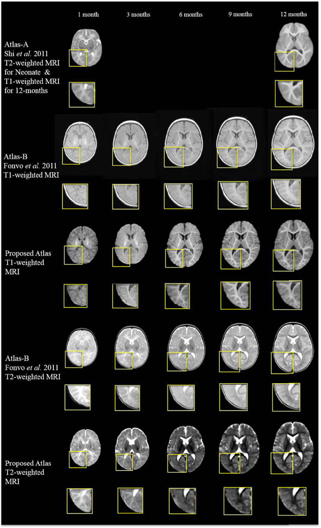
Comparison of infant longitudinal atlases constructed by Shi et al. (Atlas-A, 2011), Fonov et al. (Atlas-B, 2011), and our proposed method on the 35 aligned images (Proposed Atlas). Similar slices were selected from each of these five atlases on each time point for easy comparison. The atlases generated by the proposed method provide the clearest structural details, especially in the cortical regions shown by the close-up-views.

H. Evaluation of Atlas Representativeness

We further evaluate the 3 longitudinal atlases shown in Fig. 7 in terms of how well they can spatially normalize infant brain images. In this assessment, we use two test datasets, one from neonate population and one from 1-year-old population. Note that these datasets are independent of the subjects used for atlas construction. Dataset 1 (the neonate dataset) includes 15 neonatal images, scanned at 14 to 58 days postnatal on a 3T Siemens scanner [30]. T2 images were obtained with 87 axial slices at a resolution of 1.00 × 1.00 × 1.30mm³. Dataset 2 (the 1-year-old test set) includes 20 infant images, scanned at 87.9–109.1 gestational weeks using a Siemens 3T scanner. T1-weighted images were obtained with 160 axial slices for a resolution of 1 × 1 × 1mm³. Similar image preprocessing was performed on these two datasets, including bias correction, skull stripping, and tissue segmentation. All test images are aligned to each of the atlases by first using affine registration [31] and then nonlinear deformable registration with Diffeomorphic Demons [32], respectively. For Dataset 1, the 1-month-old atlases are used for evaluation; while for Dataset 2, images are aligned to 12-months-old atlases.

For each atlas and each dataset, a mean segmentation image is obtained by voxel-wise majority voting using all aligned segmentation images. The segmentation images of all individuals, warped to the atlas space, are then compared with this mean segmentation image by means of Dice Ratio: $DR=2|A\cap B|/(|A|+|B|)$, where A and B are the two segmentation maps. The structural agreement is calculated in pair of each aligned image and the voted mean segmentation image, which denotes the ability of each atlas for guiding and aligning test images into a common space. Statistical analysis results are shown in Fig. 8, which indicates that the proposed atlases outperform all other datasets.

Fig. 8.

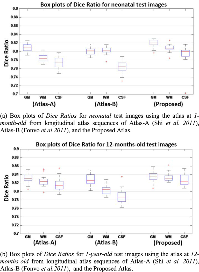
Box plots of Dice Ratio using two state-of-the-art longitudinal atlases and also the proposed atlases, respectively. The red lines in the boxes mark the medians. The boxes extend to the lower and upper quartiles (i.e., 25% and 75%). Outliers beyond this range are marked by red “+” symbols.

The effectiveness of atlas-guided normalization is further confirmed by the average normalized tissue segmentation maps of test images in Fig.9. Gray matter (GM) is distributed at the surfaces of the cerebral hemispheres (cerebral cortex) and the cerebellum (cerebellar cortex). Thus, more precise registration of cerebral cortex leads to more accurate GM maps. Fig. 9 compares the average tissue maps generated by atlas-guided normalizations, using (left column) the average 1-month-old atlas, and (right column) the proposed 1-month-old atlas as references, respectively. The tissue map in the right column, which is normalized using the proposed atlas, shows clearer cortical structures than the map in the left column. This is because the proposed atlas provides an improved detail- preserved template, thus is able to guide registration more precisely in the cerebral cortex region.

Fig. 9.

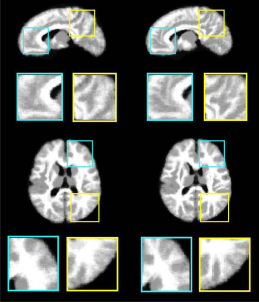
Tissue segmentation maps generated by averaging the segmentation maps of normalized test images. The normalization was performed using (left column) the average 1-month-old atlas, and (right column) the proposed 1-month-old atlas as references, respectively. The average segmentation map in the right column shows more detailed cortical structures, compared to the other segmentation map in the left column.

I. Evaluation of Longitudinal Consistency

By calculating the volume of brain tissues on each time point, we can check the tissue volume consistency across atlases. The scatter plots are shown in Fig. 10. The volumes of all these brain structures show continuous development along time. And the tissue volumes of the proposed atlases are closer to the regression curve than the average longitudinal atlases. This further indicates that the proposed method improves temporal consistency.

Fig. 10.

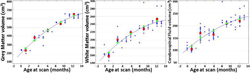
Scatter plots of brain tissue (from left to right: GM, WM and CSF) volumes against age at scan, along with quadratic regression. The blue stars represent tissue volumes of subjects, the red cubes represent volumes of mean atlases, and the green cubes represent volumes of the proposed atlases.

In order to quantitatively analyze the temporal consistency for the proposed atlas sequence, we define the temporal consistency (TC) factor. Suppose $I_{atlas}^{GM}\left(t^m\right)\text{and}{I}_{\mathit{\text{atlas}}}^{WM}\left(t^m\right)$ are the GM and WM maps for the proposed atlas on the m-th time point. According to the longitudinal deformations χ(t^m )(m = 1, ∙ ∙ ∙, M), we can estimate tissue label maps $I_{\mathit{\text{atlas}}}^{GM/WM}\left(t^m\to t^{m^{\prime }}\right)\left(m,m^{\prime }=1,\cdots ,M;m\ne m^{\prime }\right)$ on time point t^m’ by warping the label maps $I_{\mathit{atlas}}^{GM/WM}\left(t^m\right)$ of the time point t^m:

$$\begin{gathered} I_{atlas}^{GM/WM}\left(t^m\to t^{m^{\prime }}\right)=I_{atlas}^{GM/WM}{\left(t^m\right)}^{°}\chi {\left(t^m\right)}^{°}{\chi }^{-1}\left(t^{m^{\prime }}\right) \\ \left(m=1,\cdots ,M;m^{\prime }=1,\cdots ,M;m\ne m^{\prime }\right) \end{gathered}$$ (11)

Consider that $I_{atlas}^{GM/WM}\left(t^m\right)$ are the probability maps. We compute the absolute GM/WM label difference $D\left(t^m,t^{m^{\prime }}\right)=\left|I_{\mathit{\text{atlas}}}^{GM/WM}\left(t^{m^{\prime }}\right)-I_{\mathit{\text{atlas}}}^{GM/WM}\left(t^m\to t^{m^{\prime }}\right)\right|$ between the atlas map on time t^m’ and the atlas map warped from other time t^m. If for one voxel D(t^m, t^m’) > 15, we consider the label of this voxel has been changed. Denote $\begin{array}{l}Coun{t}_{t^m\to t^{m^{\prime }}}^{GM/WM}\hfill \end{array}$ as the number of voxels whose labels have been changed along the deformation from time t^m to t^m’. The temporal consistency (TC) factor can be calculated as: $TC=1-\frac{{\mathit{\text{Count}}}_{t^m\to t^{\mathrm{m\prime }}}^{\mathrm{GM}/\mathrm{WM}}}{Vol(GM/WM)}$ where Vol(GM/WM) represents the volume of a tissue map. Thus, TCs of GM and WM reflect the temporal consistency of the tissue maps. Higher values indicate relatively better temporally consistent results. Tables T2–T3 in the supplementary materials (available in the supplementary files /multimedia tab) show the TCs of GM and WM of the entire brains, calculated from the average atlas sequence and the proposed atlas sequence. It can be seen that the improvements are significant.

IV. DISCUSSION

Regarding the applications, atlas construction studies could be broadly clustered into two categories. The first category includes works focusing on describing the averaged anatomy, i.e., common brain structures in a standardized space. It provides a useful reference for combination and comparison of brain mapping findings. Typical examples include the ICBM atlas [33], JHU DTI-based white-matter atlases [34], and non-linear MNI152 atlas [4]. Our work also belongs to this category. In the second category, atlas is used to trace the individual variations in population, which is commonly applied in the disease related atlas studies. For example, Thompson et al. [35] built a statistic model for Alzheimer Disease, where the authors show the statistically different brain tissue variations between normal controls and patient group. Ye et al. provide in [36] an iron-elevation variation study among Parkinson’s disease patients based on quantitative susceptibility mapping. It provides useful information to accurately characterize specific variations while taking into account the inter-individual variability.

The temporal-consistent constraint in the proposed method is typically designed for our longitudinal data precisely scanned for similar number of time-points and age range. For extending this to solve more general problems, such as aging study where the observation period varies across individuals, our future work would consider using regression model or Gaussian kernel to estimate the unmatched time-points.

V. CONCLUSION

In this paper, we propose a novel patch-based longitudinal atlas construction method by simultaneous consideration of both subject-specific longitudinal variability and inter-subject variability. Specifically, our approach employs a grouped local refinement strategy in constructing serial atlases to ensure spatial and temporal consistency. This is confirmed by various experimental results, demonstrating that our approach yields longitudinal atlases with greater temporal consistency and gives better performance in infant image normalization compared with two state-of-the-art infant longitudinal atlases. The algorithm and atlases will be publicly available in our website, http://bric.unc.edu/ideagroup/free-softwares/.

REFERENCES

- [1].Knickmeyer RC et al. , “A structural MRI study of human brain development from birth to 2 Years,” J. Neurosci, vol. 28, no. 47, pp. 12176–12182, 2008. [DOI] [PMC free article] [PubMed] [Google Scholar]
- [2].Shi F et al. , “Infant brain atlases from neonates to 1- and 2-year-olds,” PLoS ONE, vol. 6, no. 4, p. e18746, 2011. [DOI] [PMC free article] [PubMed] [Google Scholar]
- [3].Kuklisova-Murgasova M et al. , “A dynamic 4D probabilistic atlas of the developing brain,” Neuroimage, vol. 54, no. 4, pp. 2750–2763, 2011. [DOI] [PubMed] [Google Scholar]
- [4].Fonov V et al. , “Unbiased average age-appropriate atlases for pediatric studies,” Neuroimage, vol. 54, no. 1, pp. 313–327, 2011. [DOI] [PMC free article] [PubMed] [Google Scholar]
- [5].Serag A et al. , “Construction of a consistent high-definition spatiotemporal atlas of the developing brain using adaptive kernel regression,” Neurolmage, vol. 59, no. 3, pp. 2255–2265, 2012. [DOI] [PubMed] [Google Scholar]
- [6].Habas PA et al. , “A spatiotemporal atlas of MR intensity, tissue probability and shape of the fetal brain with application to segmentation,” Neurolmage, vol. 53, no. 2, pp. 460–470, 2010. [DOI] [PMC free article] [PubMed] [Google Scholar]
- [7].Jin Y et al. , “Automatic clustering of white matter fibers in brain diffusion MRI with an application to genetics,” Neuroimage, vol. 100, pp. 75–90, October 2014. [DOI] [PMC free article] [PubMed] [Google Scholar]
- [8].Fishbaugh J, Prastawa M, Gerig G, and Durrleman S, “Geodesic shape regression in the framework of currents,” in inf. Process. Med. imag.. pp. 718–729. [DOI] [PMC free article] [PubMed] [Google Scholar]
- [9].Xie Y, Ho J, and Vemuri BC, “Multiple atlas construction from a heterogeneous brain MR image collection,” iEEE Trans. Med. imag., vol. 32, no. 3, pp. 628–635, March 2013. [DOI] [PMC free article] [PubMed] [Google Scholar]
- [10].Davis BC, Fletcher PT, Bullitt E, and Joshi S, “Population shape regression from random design data,” int. J. Comput. Vis, vol. 90, no. 2, pp. 255–266, 2010. [Google Scholar]
- [11].Dittrich E et al. , “A spatio-temporal latent atlas for semi-supervised learning of fetal brain segmentations and morphological age estimation,” Med. image Anal, vol. 18, no. 1, pp. 9–21, 2014. [DOI] [PubMed] [Google Scholar]
- [12].Oishi K et al. , “Multi-contrast human neonatal brain atlas: Application to normal neonate development analysis,” Neuroimage, vol. 56, no. 1, pp. 8–20, 2011. [DOI] [PMC free article] [PubMed] [Google Scholar]
- [13].Gholipour A et al. , “Construction of a deformable spatiotemporal MRI atlas of the fetal brain: Evaluation of similarity metrics and deformation models,” in Medical image Computing and Computer-Assisted intervention. New York: Springer, 2014, pp. 292–299. [DOI] [PMC free article] [PubMed] [Google Scholar]
- [14].Durrleman S, Pennec X, Trouvé A, Gerig G, and Ayache N, “Spatiotemporal atlas estimation for developmental delay detection in longitudinal datasets,” Medical image Computing and Computer-Assisted intervention. New York: Springer, 2009, pp. 297–304. [DOI] [PMC free article] [PubMed] [Google Scholar]
- [15].Liao S, Jia H, Wu G, and Shen D, “A novel framework for longitudinal atlas construction with groupwise registration of subject image sequences,” Neuroimage, vol. 59, no. 2, pp. 1275–1289, 2012. [DOI] [PMC free article] [PubMed] [Google Scholar]
- [16].Liu M, Zhang D, and Shen D, “Relationship induced multi-template learning for diagnosis of Alzheimer’s disease and mild cognitive impairment,” iEEE Trans. Med. imag, vol. 35, no. 6, pp. 1463–1474, June 2016. [DOI] [PMC free article] [PubMed] [Google Scholar]
- [17].Shi F et al. , “Neonatal atlas construction using sparse representation,” Human Brain Map, vol. 35, no. 9, pp. 4663–4677, 2014. [DOI] [PMC free article] [PubMed] [Google Scholar]
- [18].Zhang Y, Shi F, Yap P-T, and Shen D, “Space-frequency detail-preserving construction of neonatal brain atlases,” in Proc. MiCCAi, 2015, pp. 255–262. [DOI] [PMC free article] [PubMed] [Google Scholar]
- [19].Wright R et al. , “Automatic quantification of normal cortical folding patterns from fetal brain MRI,” Neuroimage, vol. 91, pp. 21–32, May 2014. [DOI] [PubMed] [Google Scholar]
- [20].Wei H et al. , “Free-breathing diffusion tensor imaging and tractography of the human heart in healthy volunteers using wavelet-based image fusion,” iEEE Trans. Med. imag, vol. 34, no. 1, pp. 306–316, January 2015. [DOI] [PubMed] [Google Scholar]
- [21].Wei H et al. , “Assessment of cardiac motion effects on the fiber architecture of the human heart in vivo,” iEEE Trans. Med. imag, vol. 32, no. 10, pp. 1928–1938, October 2013. [DOI] [PMC free article] [PubMed] [Google Scholar]
- [22].Smith SM et al. , “Advances in functional and structural MR image analysis and implementation as FSL,” Neuroimage, vol. 23, pp. S208–S219, 2004. [DOI] [PubMed] [Google Scholar]
- [23].Shi F et al. , “LABEL: Pediatric brain extraction using learning-based meta-algorithm,” Neuroimage, vol. 62, no. 3, pp. 1975–1986, 2012. [DOI] [PMC free article] [PubMed] [Google Scholar]
- [24].Shen D and Davatzikos C, “HAMMER: Hierarchical attribute matching mechanism for elastic registration,” iEEE Trans. Med. imag, vol. 21, no. 11, pp. 1421–1439, November 2002. [DOI] [PubMed] [Google Scholar]
- [25].Sled JG, Zijdenbos AP, and Evans AC, “A nonparametric method for automatic correction of intensity nonuniformity in MRI data,” iEEE Trans. Med. imag, vol. 17, no. 1, pp. 87–97, February 1998. [DOI] [PubMed] [Google Scholar]
- [26].Wang L et al. , “4D multi-modality tissue segmentation of serial infant images,” PLoS ONE, vol. 7, no. 9, p. e44596, 2012. [DOI] [PMC free article] [PubMed] [Google Scholar]
- [27].Wu G, Wang Q, Jia H, and Shen D, “Feature-based groupwise registration by hierarchical anatomical correspondence detection,” Human Brain Map, vol. 33, no. 2, pp. 253–271, 2012. [DOI] [PMC free article] [PubMed] [Google Scholar]
- [28].Liu J, Ji S, and Ye J, “Multi-task feature learning via efficient l2 1-norm minimization,” in Proc. 25th Conf. Uncertainty Artif. intell, 2009, pp. 339–348. [Google Scholar]
- [29].Zhang Y, Shi F, Yap P-T, and Shen D, “Detail-preserving construction of neonatal brain atlases in space-frequency domain,” Human Brain Map, vol. 37, no. 6, pp. 2133–2150, 2016. [DOI] [PMC free article] [PubMed] [Google Scholar]
- [30].Shi etal F., “CENTS: Cortical enhanced neonatal tissue segmentation,” Human Brain Map, vol. 32, no. 3, pp. 382–396, 2011. [DOI] [PMC free article] [PubMed] [Google Scholar]
- [31].Jenkinson M, Bannister P, Brady M, and Smith S, “Improved optimization for the robust and accurate linear registration and motion correction of brain images,” Neuroimage, vol. 17, no. 2, pp. 825–841, 2002. [DOI] [PubMed] [Google Scholar]
- [32].Vercauteren T, Pennec X, Perchant A, and Ayache N, “Diffeomorphic demons: Efficient non-parametric image registration,” Neuroimage, vol. 45, no. 1, pp. S61–S72, 2009. [DOI] [PubMed] [Google Scholar]
- [33].Mazziotta J et al. , “A probabilistic atlas and reference system for the human brain: International consortium for brain mapping (ICBM),” Phil. Trans. R. Soc. London B, Biol. Sci., vol. 356, no. 1412, pp. 1293–1322, 2001. [DOI] [PMC free article] [PubMed] [Google Scholar]
- [34].Hua K et al. , “Tract probability maps in stereotaxic spaces: Analyses of white matter anatomy and tract-specific quantification,” Neuroimage, vol. 39, no. 1, pp. 336–347, 2008. [DOI] [PMC free article] [PubMed] [Google Scholar]
- [35].Thompson PM et al. , “Cortical variability and asymmetry in normal aging and Alzheimer’s disease,” Cerebral Cortex, vol. 8, no. 6, pp. 492–509, 1998. [DOI] [PubMed] [Google Scholar]
- [36].He N et al. , “Region-specific disturbed iron distribution in early idiopathic Parkinson’s disease measured by quantitative susceptibility mapping,” Human Brain Map, vol. 36, no. 11, pp. 4407–4420, 2015. [DOI] [PMC free article] [PubMed] [Google Scholar]
- [37].Dai Y, Shi F, Wang L, Wu G, and Shen D, “iBEAT: A toolbox for infant brain magnetic resonance image processing,” Neuroinformatics, vol. 11, no. 2, pp. 211–225, 2013. [DOI] [PubMed] [Google Scholar]
Associated Data
This section collects any data citations, data availability statements, or supplementary materials included in this article.