Automated Vision-Based High Intraocular Pressure Detection Using Frontal Eye Images

Abstract

Glaucoma, the silent thief of vision, is mostly caused by the gradual increase of pressure in the eye which is known as intraocular pressure (IOP). An effective way to prevent the rise in eye pressure is by early detection. Prior computer vision-based work regarding IOP relies on fundus images of the optic nerves. This paper provides a novel vision-based framework to help in the initial IOP screening using only frontal eye images. The framework first introduces the utilization of a fully convolutional neural (FCN) network on frontal eye images for sclera and iris segmentation. Using these extracted areas, six features that include mean redness level of the sclera, red area percentage, Pupil/Iris diameter ratio, and three sclera contour features (distance, area, and angle) are computed. A database of images from the Princess Basma Hospital is used in this work, containing 400 facial images; 200 cases with normal IOP; and 200 cases with high IOP. Once the features are extracted, two classifiers (support vector machine and decision tree) are applied to obtain the status of the patients in terms of IOP (normal or high). The overall accuracy of the proposed framework is over 97.75% using the decision tree. The novelties and contributions of this work include introducing a fully convolutional network architecture for eye sclera segmentation, in addition to scientifically correlating the frontal eye view (image) with IOP by introducing new sclera contour features that have not been previously introduced in the literature from frontal eye images for IOP status determination.

We present a novel and effective method for early detection of high intraocular pressure, which is the leading cause of glaucoma, the silent thief of vision. Our vision-based framework can screen for high intraocular pressure using only frontal eye images.

I. Introduction

Glaucoma is known as the silent blinding disease. It is one of the leading causes of blindness worldwide. In many cases, due to increased intraocular pressure (IOP), the optic nerve is damaged, vision is reduced, and the final result is Glaucoma [1]. The blindness caused by Glaucoma is irreversible as the optic nerve dies [2]. One effective way to prevent and control blindness from Glaucoma is through early detection [3]. The earlier the disease is detected, the easier and more effective the treatment will be.

In an initial diagnosis, patients are referred to as Glaucoma candidates [4]. In most cases, this damage is found in candidates due to increased pressure within the eye. The eye produces a fluid called aqueous humor which is secreted by the ciliary body into the posterior chamber (a space between the Iris and the lens) [5]. Then, it flows through the Pupil into the anterior chamber between the Iris and the cornea [6]. From here, it drains through a sponge-like structure located at the base of the Iris called the trabecular meshwork [7], and then leaves the eye. In a healthy eye, the rate of secretion balances the rate of drainage [8]. In Glaucoma candidates, the drainage canal is partially or completely blocked. Fluid builds up in the chambers and causes an increase of pressure within the eye [9]. The pressure drives the lens back and presses on the vitreous body, which in turn compresses and damages the blood vessels and nerve fibers running at the back of the eye. These damaged nerve fibers result in patches of vision loss, and if left untreated, may lead to total blindness [10].

IOP is generally determined by regular eye exams such as Tonometry test, Ophthalmoscopy test, Perimetry test, Gonioscopy test, and Pachymetry test, where the patient needs to visit the clinic and medical staff/personnel have to be present to perform the tests/measurements [11], [12].

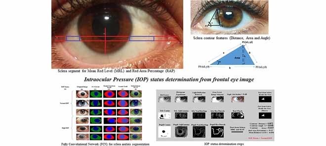
In this paper, a novel preliminary intraocular pressure detection framework is developed to aid patients in their monthly clinic visits by enabling doctors/individuals to initially monitor the patients’ eye pressure risk by non-contact means, non-invasively. The proposed approach is based on vision and machine-learning techniques where a fully convolutional neural network (an instance of deep learning) is introduced for sclera and iris segmentation from frontal eye images. Six features are then extracted from the segmented areas. These features are the Pupil/Iris diameter or radius ratio, the Mean Redness Level (MRL) and Red Area Percentage (RAP) of the sclera, and three features from the contour of the sclera (area, distance and angle). Once the six features are extracted from all images, a binary classifier will be applied in order to train and test the images to obtain the risk assessment result for intraocular pressure. It is important to mention that no previous research studied frontal eye images to determine the status of IOP for initial screening. Therefore, this research provides a completely novel idea in this field.

Building over our work in [13], [14], this research studies several algorithms and certain algorithms are selected to direct this research to be automated such that it can eventually be applied on smart-phones. The main contributions of the proposed work can be specified in the following points:

• •Proposing a new framework to help both ophthalmologists and high IOP candidates in the initial diagnosis of IOP early-on, as it is the most effective approach to prevent full or partial IOP/Glaucoma based vision loss.
• •Introducing a novel vision-based architecture, structure and features for initial IOP screening using frontal eye images. This work shows that there is evidence of computational relationship between the IOP status and frontal eye image features. New sclera contour features are presented in this work that have not been previously introduced in the literature from frontal eye images for IOP status determination.
• •Introducing a new application for the Fully Convolution Neural Network (FCNN) in sclera and iris detection and segmentation.
• •Enhancing the classification performance by applying the Decision Tree (DT) classifier for the area extracted from the improved sclera segmentation.

The rest of the paper is organized as follows: Section II discusses other prior related work on computer vision based or automated IOP and Glaucoma detection. The proposed framework is introduced in Section III. In Sections IV and V, the detailed design scheme is presented, and the results, comparisons and efficiency tests are described. Finally, Section VI concludes this paper and presents future directions.

II. Related Work

Many researchers have proposed several works for IOP and Glaucoma detection and analysis of the eye from images. However, there is a lack of studies regarding IOP based on frontal eye images in the computer vision field.

Yousefi et al. [15] worked on fundus images to demonstrate a pipeline to cluster the visual field into two categories, normal and Glaucoma. The Glaucoma category was clustered into two patterns, the stable and the progression. The authors modeled the visual field data using the mixture of Gaussians approach and the Generalized Expectation Maximization (GEM) technique. The authors in [16] also provided a method for Glaucoma progression detection using Machine Learning Classifiers (MLC’s) from fundus images. The optic disc images and the thickness of the surrounding retinal nerve fiber layer were taken by using the Optical Coherence Tomography (OCT). A combination of several classifiers such as Bayesian, Instance-based, Meta, and tree families of MLC’s plus Bayesian net were used. The accuracy of their work was reported as 88%.

Mariakakis et al. [17] proposed an approach to assess intraocular pressure using a smart-phone with a hardware adapter. The adapter is a clear acrylic cylinder with a diameter of 8 mm and height of 63 mm that is connected to the camera of the smart-phone. A trained user would hold the smart-phone perpendicularly over the patient’s eye and then applies the weight of the acrylic cylinder to it. The smart-phone camera would then start recording the applanation of the eye. Video analysis is then applied to measure two ellipses, the acrylic cylinder (outer ellipse) and the applanation surface (inner ellipse). The ellipses are then mapped to absolute measurements of the diameter of the acrylic cylinder. The final diameter measurement is mapped to an IOP value using a clinically validated table such as the one published by Posner [18]. The authors reported an accuracy of 89% regarding their work. This device, however, cannot be deployed by ordinary users; the patient must visit the clinic and only specialists can operate the device.

The authors in [19] proposed a wireless powered on-lens IOP monitoring system. The system consists of an on-lens capacitive sensor, a read-out circuit and radio frequency identification (RFID) system. The proposed sensor establishes communication with an on-glass reader and measures the on-lens capacitance changes through the microelectromechanical system capacitive sensor. The distance between the glass and the contact lens is about 2 cm. In order to maintain the communication between the glass and the lens using low-power RF, the antenna should be kept within the area of 1.6 cm². To use this system, the user must wear a glass and a lens sensor at the same time along with an RFID reader around the neck, which may not be convenient for all patients. Additionally, Santiago et al. [20] proposed a system for measuring IOP using a resonant sensor. A comparison between magnetic and resonant sensors was made. It was shown that resonant sensors provide more promising results according to the changes that were measured on the impedance of a test coil due to the changes of the capacitance of the sensor. The IOP value was obtained from the measured resonance frequency by extracting the real part of the input impedance of the external coil as a function of frequency [21].

All prior related work either focus on fundus/optic disc images or additional hardware sensors for eye blood vessel detection and IOP/Glaucoma determination, or Pupil/ Iris detection and/or eye redness determination from frontal eye images for applications other than IOP and Glaucoma [1]–[4]. The proposed framework is intended to serve as an initial step for IOP screening for any user, especially those with family history of high IOP and Glaucoma. It is not intended to replace the state-of-art frameworks, because clearly the inputs and even outputs are different, and therefore a fair comparison cannot be made. The input of our framework is the frontal eye image and the output is a binary decision whether the eye is at normal or high IOP. To the best of our knowledge, IOP risk assessment from purely frontal eye images has not been reported to date.

III. Methods and Procedures

In this paper, an initial IOP risk assessment framework is developed based on frontal eye images. A fully convolutional network is proposed in the framework for sclera and Iris segmentation. From these segmented areas, six features are extracted. The final results of the risk grade level of IOP are based on machine learning techniques using decision tree and support vector machine classifiers. The implementation is carried out using MATLAB 2014a software.

A. Dataset

In this study, the image database¹¹ (DB) from the Princess Basma Hospital (Jordan-Irbid) is utilized in which four hundred individuals participated. Half of them were patients with high eye pressure. The other half of the participants represented normal eye pressure cases. There was a total of 244 male and 156 female participants. The age range of the participants fell between 40 and 65 years old. Each participant’s level of eye pressure was recorded in the database and labeled as normal/high eye pressure by the ophthalmologists. The IOP ranges of the normal eye pressure cases were 11–21 mmHg, while the range of high IOP cases were greater and in the range of 22–30 mmHg [10], [22]. All the database images were taken in a range of 20 cm between the camera and the participants. A canon camera model T6 K1 with a resolution of was used to take the images. All eye images were taken in the same lightning conditions and saved in a consistent format.

B. Eye Segmentation and Feature Extraction

To build a framework for IOP risk assessment determination, the database of images was trained. The proposed system is implemented using real-time face detection and tracking based on the Adaboost face detection algorithm and Haar cascade eye detection techniques [23], [24]. The color format used to represent the image in each frame is RGB. The Haar cascade technique [25], [26] was used to extract the left and right eyes. Each eye area segment was extracted as a rectangle.

1). Extracting the Sclera

Sclera segmentation is a challenging process, especially that in cases of high IOP, Cataract and Glaucoma, most of the sclera area becomes red. For that reason, a robust segmentation algorithm is required that can handle such cases. In the last couple of years, deep learning with convolutional neural networks (CNN) have shown promising results in semantic segmentation for objects [27]–[31]. Most of these network structures are complicated and time consuming, especially to be implemented on smart-phone devices. In this paper, a modified version of the fully convolution network (FCN) structure in [27] is introduced for its simplifications over other structures. The proposed FCN consists of convolutional layers for feature extraction without any fully connected layers. At the later stages of the network, deconvolutional layers are used to resize the image back to its original size. The network structure of the proposed network is represented in Figure 1. To improve segmentation edges, the last stage results are added to early stages to use the edge features generated in the early stages. As shown in the Figure, each convolution stage includes a Rectified Linear Unit (ReLU) activation function, and at the end of each stage, maximum pooling is used to down sample the extracted images. Section IV will include a sample of the results for this trained network versus applying previously used Hough transform for sclera segmentation.

FIGURE 1.

Fully Conventional Network (FCN) structure for sclera segmentation.

2). Extracting the Pupil/Iris Ratio

After extracting the desired eye, the Height:Width ratio is set to be 1:1.8, respectively. The automated resizing process is applied to the image so that the height would equal 150 pixels. Then, the red layer image is selected because it discards unwanted data and enhances the Iris and the Pupil area. After that, histogram equalization is applied to enhance the contrast of the Iris and Pupil area. A morphological reconstruction technique [32] is then applied to remove the light reflection on the Pupil. Moreover, adaptive thresholding [33] is applied to separate the foreground from background in order to extract the gray level range containing the Iris and the Pupil. Finally, as a preprocessing stage, canny edge detection technique is applied to detect the edges of the Pupil and the Iris. Canny edge technique, in its nature, contains non-max suppression [34] and Hysteresis thresholding [35]. After the above preprocessing, the Circular Hough Transform (CHT) technique [36], [37] is applied in order to detect the Iris and then the Pupil, where the Pupil/Iris radius (or diameter) ratio is also computed.

3). Pure Red Color Selection

After cropping a targeted portion of the sclera, extended from two horizontal lines at one third and half of the lower vertical radius of the Iris (Figure 2(a)), the MRL and RAP features are calculated (Figure 2(b)). The MRL is heavily based on the red pixel value. Each pixel is a combination of three values (Red, Green, and Blue). In addition, there are several cases that can result in reddish colors if we assign a large value to the red part of the pixel. Therefore, the red pixel value should always be larger than the green and blue pixel values. To prevent the pixel from being shifted to the yellow or violet colors, the difference between the green and the blue pixel values should not be too large. As per Table 1, different ranges of the redness level of the eye are identified by the closest color to the pure red value.

FIGURE 2.

Extracting sclera and calculating MRL/RAP features.

TABLE 1. Ratio of Red Colors.

Color	RPV	GPV	BPV	MRL
Reddish1	255	200	200	0.477124
Reddish2	255	100	100	0.738562
Reddish3	255	50	50	0.869281
Pure Red	255	0	0	1
Reddish4	180	75	75	0.509804
Reddish5	180	50	50	0.575163
Reddish6	180	25	25	0.640523
Pure Dark Red	180	0	0	0.705882

4). Mean Redness Level (MRL)

IOP takes a long time to start affecting the eye vision in the case of Primary Open Angle Glaucoma (POAG). However, in acute angle-closure, the pressure increases suddenly, and it only takes hours to have high IOP. This sudden rise affects the eye in different parts. For instance, the eye becomes red and the cornea clouds and swells [38]. Therefore, it is important to cover the long-term and short-term chances of having high IOP by measuring the redness of the sclera through the mean redness level (MRL).

Based on the ranges of red pixel values, the Mean Redness Level (MRL) can be calculated by the proposed Equation 4:

Then,

where corresponds to the mean of the red pixel value, is the mean of the green pixel value, and is the mean of blue pixel value. The coefficient value of 3 is selected due to the fact that there are three channels. By using the color pixel values found in Table 1, the MRL ratio is calculated and displayed in the last column of Table 1.

The MRL and RAP features are calculated from Image () from the extracted portion of the sclera. This portion is created by constructing a black image that has the same size of the merged extracted portions of the sclera which is Image (), as shown in Figure 2(b). The colored image is then scanned pixel by pixel. Every time a red value is located, the black image pixel value is modified into a white pixel value.

5). Red Area Percentage (RAP)

As seen in Figure 2, MRL and RAP are computed from the extracted portion of the sclera. In our framework, the RAP feature is defined as the mean of the red pixel percentage in the binary image.

In Equation 5, represents the red pixel values in the region of interest extracted from the sclera, and represents the total number of pixels in that region. Figure 2(b) represents a sample of the MRL and RAP values from a frontal eye image.

6). Contour Features (Area, Distance, Angle)

The idea of measuring three features from the extracted contour of the sclera is inspired by sonar techniques such as ultrasound where traditionally, the thickness of the cornea liquid is measured by active trained operators/healthcare personnel who scan certain points of the eye [39]. The newly proposed strategy is automated and works by scanning the area of the eye shown in Figure 3, where the contour is extracted using the active contour model [40] to calculate the Distance (), Angle (), and Area. These are newly proposed features from frontal eye images that have not been previously investigated in the literature for IOP.

FIGURE 3.

DEpiction of distance (), angle () and area features of the contour of the sclera.

To automatically compute the , and Area sclera contour features, as shown in Figures 3 and 4, the triangle consisted of points , , with three sides , , and is considered. The height (), Area, and angle () can be found from the triangle. The coordinates of points and P2 can be found from the border of the Iris for the left and right eyes (Equations 6–11).

FIGURE 4.

Distance (), Angle () and Area measurements.

Moreover, is also a known point from the horizontal line illustrated in the MRL section, which is the midpoint between the left/right border of the image and (which is considered as the left/right border of the Iris) for the left/right eyes (Equations 12–14).

where,

and,

where,

and,

where,

Therefore,

where is the radius of the Iris, and and represent the coordinates of the center of the Iris.

After identifying the coordinates of points , and , Equations 15–19 depict the steps to compute the three sclera contour features Distance (), Angle () and Area. The length of the side (which is ) is almost the same size of the diameter of the Iris after applying Equation 17. The height () can be found by moving pixel by pixel from the coordination of point across the y axis until reaching the base (). Once we reach the base (), the coordination is known and the length of the height () is calculated. The Angle (), and Area can thus be computed from Equations 18 and 19.

IV. Results

The objective of this study is to extract features from frontal eye images in an effort to determine the status of high risk IOP. Initially, the segmentation process and the results of each feature is presented separately.

A. Sclera Segmentation

The segmentation technique proposed in Section III is implemented using the Caffe toolbox with Python wrapper on an Nvidia Titan x GPU. Since the sclera segmentation process should work with any frontal eye image (with or without eye diseases), the collected dataset images along with other normal IOP frontal eye images collected over the internet (such as the images from the publicly available databases used in [41]) are combined (normal and high IOP) and divided into two groups, training and testing groups. To increase the number of images in the dataset, data augmentation techniques have been used by 2D transformations of the eye images. Moreover, all images utilized in the FCN training process have been inspected and manually labeled to mark the Iris and Pupil areas to generate the ground-truth dataset for the learning algorithm. The total number of images achieved for this segmentation process is 858 images from different people of various races. Half of these images are used for training and the other 50% are used for testing. The weights of the designed network are initialized by transfer learning from the segmentation network designed in [29]. Softmax loss function is used and solved with the Stochastic Gradient Decent optimization (SGD) technique. Results of the proposed network for segmentation can be found in Table 2. Mean accuracy, pixel accuracy (overall accuracy) and region intersection of union (IU) are used as metric results for the segmentation process. Formulations for these metrics are presented in Equations 20–22. Examples for the FCN segmentation results are shown in Figure 5. As can be seen from the Figure, the proposed FCN network shows better results and improved segmentation performance over Hough transform, as used in [13], [41].

where is the number of pixels correctly predicted to be in class , and is the number of pixels predicted to be in class , while they actually belong to class . is the number of predicted classes. is the total number of pixels that belong to class .

TABLE 2. Segmentation Metrics.

Mean Accuracy	94.4
Overall Accuracy	92.3
Mean IU	63.4

FIGURE 5.

Sclera and Iris segmentation (a) IOP Status; (b) Original Image; (c) FCN Result; (d) Hough transform Result; (e) Ground-truth; (f) Masked Image from FCN.

Other segmentation techniques such as the one introduced in [41], rely on a shape model similar to the Active Shape Model (ASM) technique used for face landmarks detection. A look-up table is used based on the sclera color from the training images using a support vector machine (SVM) to generate the probability that a given pixel is a sclera or not. Such techniques, however, are not suitable for sclera segmentation in our initial IOP screening framework.

In terms of computational complexity, FCN consists of multiple convolutional processes as a function of size and features, so the best complexity is , while the Hough transform, which was used in [13], has a best complexity of O() as a function of the size of each dimension. The computational complexity of [41] depends on the algorithm used in the optimization process of the shape model + the complexity of the RBF based SVM, which can be represented as , because the number of training images are larger than the number of features, where n is the number of sample images and d is the number of features used with the SVM classifier. Taking into consideration that the proposed system is most competently designed for personal home use for IOP status detection (without professional/clinical assistance), FCN will be a great choice, especially on the new neural processors utilized in modern smart-phones, which will reduce the execution time for the FCN compared to other techniques, that run over a regular CPU with higher complexity.

B. Pupil/Iris Ratio

During the day, a normal adult’s Pupil/Iris diameter varies (between 2 mm to 4 mm for the Pupil and 11 mm to 14 mm for the Iris [42]). Traditionally, the radius of the Iris and Pupil is measured in millimeters. However, according to computer vision, it is inaccurate to represent the radius in millimeters even when images contain information such as fixed distance and tangible objects. Therefore, in this study we rely on both the Iris and the Pupil to calculate the ratio for accurate results because the units will be discarded. In our study, the ratio of the Pupil/Iris in daytime hours fall between (0.45, 0.70) for adults. Table 3 represents a sample of the results after our Pupil/Iris ratio detection technique was applied to the frontal eye images. The table is split into two blocks. The first block shows the results for normal IOP cases; the second block shows the results for eyes with high pressure. Each block contains a sample of the results for the Pupil/Iris ratio, as well as the MRL and RAP features. The average (AVG) of all normal and high IOP cases is also listed.

TABLE 3. Sample of Pupil/Iris Ratio, MRL and RAP Feature Values for Normal and High IOP Cases.

Normal			High pressure
Pupil/Iris Ratio	MRL	RAP	Pupil/Iris Ratio	MRL	RAP
0.53	0.13	0.32	0.81	0.56	0.86
0.59	0.11	0.27	0.79	0.57	0.76
0.55	0.08	0.06	0.80	0.63	0.86
	.
AVG = 0.45	AVG = 0.29	AVG = 0.19	AVG = 0.70	AVG = 0.69	AVG = 0.84

The results in Table 3 indicate that there is a strong relationship between the Pupil/Iris ratios and high intraocular pressure. This technique will help in the initial screening of IOP that may lead to early detection of high IOP, in an effort to circumvent the onset of blindness.

C. MRL and RAP

The extraction of the sclera was the most difficult part of this research, since the sclera shares the same features of the skin. Mean Redness Level was calculated according to the proposed Equation 4. Red Area Percentage was also calculated as the average of the red pixels in the extracted part of the sclera, as shown in Equation 5. Table 3 also contains a sample of the results for normal and high eye pressure cases based on the MRL and RAP features, numerically. The results show that there is a big difference between normal cases and cases with high eye pressure. This information will also, aid in automatic IOP screening for early detection of IOP, in an effort to help in preventing the blindness.

D. Features of the Sclera

In this section of the results, we report the , , and Area feature values of the sclera contour for normal and high eye pressure cases from frontal eye images of the database. Table 4 depicts these results. The contour features have been normalized as follows:

Contour Angle values cannot exceed 45° degree, which makes the maximum value in radion as 0.785.

To calculate any of these proposed features, one must go through all the pixels in the image, which will make the complexity for these features O(m n), where and are the dimensions of the extracted eye area. This complexity can be actually considered as a constant value because the size of the processed eye image will be constant throughout the features calculation process, and will thus, reduce the features overhead calculation.

TABLE 4. Contour of the Sclera Feature Values for Normal and High Intraocular Pressure Cases.

Normal			High pressure
D (Contour Distance/Iris radius)	Area (Contour Area/Iris Area)	(Radion)	D (Contour Distance/Iris radius)	Area (Contour Area/Iris Area)	(Radion)
0.0690	0.9844	0.6511	0.0132	0.1232	0.0234
0.0569	0.7466	0.8380	0.0148	0.3466	0.1343
0.0872	0.6415	0.6450	0.0230	0.0324	0.5622
0.0725	0.7454	0.7581	0.0262	0.0734	0.0324
0.0501	0.7058	0.6248	0.0362	0.0973	0.0231
AVG = 0.0723	AVG = 0.7129	AVG = 0.7387	AVG = 0.0178	AVG = 0.1079	AVG = 0.1588

E. IOP Risk Determination

Once we extracted all six features from the images, a binary classifier is applied to the extracted features in order to classify the images for an initial screening of IOP risk assessment by distinguishing normal from high IOP.

Several machine learning algorithms were applied on the extracted features. For instance, support vector machine (SVM) was tested along with the Decision Tree (DT) classifier to pick the best accuracy (Tables 5–9). For SVM, different kernels have been utilized, but only the radial basis function (RBF) kernel would converge. In this work, the decision tree classifier shows better accuracy over SVM. Therefore, DT has been used in the rest of this work. 75% of the eye images in the database are utilized for training and validation (65% training and 10% validation) and 25% are used for testing the classifiers. The binary decision tree classifier is applied to the six extracted features using the CART (Classification And Regression Tree) algorithm [43]. The output design of the tree with the following settings yielded the best results over several testing structures. The total number of nodes is 31 arranged in 6 layers of depth. The final output of our framework is either normal or high IOP. After applying the decision tree, a loss of 0.0615 has been achieved with 10-fold cross validation. The constructed decision tree structure is depicted in Figure 6. These noted specifications yield the best performances and accuracies over several trials and experiments. Figures 7(a) and (b) in the Appendix (Appendix A) represent two samples, one with normal eye pressure and another with high eye pressure based on clinical ground-truth, and after applying the proposed techniques to the eye images. The results show that the system was able to provide the same outcome. The framework is fully automated. Once the user inserts an image, the FCN segmentation is performed, all features are extracted and the status of IOP will be determined. The final result “Status of IOP” comes from the DT classifier.

TABLE 5. Training Phase Confusion Matrix for DT 65% of the Data.

		Normal	High Pressure
OUTPUT CLASS	Normal	123	3
	High Pressure	2	132
	TARGET CLASS
	Accuracy	98.4%	97.8%	Overall Acc.: 98.1%
	Error	1.6%	2.2%	Overall Err.: 1.9%

TABLE 6. Validation Phase Confusion Matrix for DT 10% of the Data.

		Normal	High Pressure
OUTPUT CLASS	Normal	18	1
	High Pressure	0	21
	TARGET CLASS
	Accuracy	100.0%	95.45%	Overall Acc.: 97.73%
	Error	0%	4.5%	Overall Err.: 2.25%

TABLE 7. Test Phase Confusion Matrix for DT 25% of the Data.

		Normal	High Pressure
OUTPUT CLASS	Normal	55	1
	High Pressure	2	42
	TARGET CLASS
	Accuracy	96.49%	97.67%	Overall Acc.: 97.08%
	Error	3.5%	2.3%	Overall Err.: 2.9%

TABLE 8. Overall Confusion Matrix for DT 100% of the Data.

		Normal	High Pressure
OUTPUT CLASS	Normal	196	5
	High Pressure	4	195
	TARGET CLASS
	Accuracy	98.0%	97.5%	Overall Acc.: 97.75%
	Error	2.0%	2.5%	Overall Err.: 2.25%

TABLE 9. Overall Confusion Matrix for SVM.

		Normal	High Pressure
OUTPUT CLASS	Normal	188	14
	High Pressure	12	186
	TARGET CLASS
	Accuracy	94.0%	93.0%	Overall Acc.: 93.5%
	Error	6.0%	7.0%	Overall Err.: 6.5%

FIGURE 6.

The constructed decision tree.

FIGURE 7.

Sample image segmentation, feature extraction and classification for (a) Normal eye pressure, and (b) High IOP.

A deep look into final structure of the used DT (Figure 6), provides an idea about the most efficient features from the introduced ones. As shown in Figure 6, the most discriminant feature is feature number 6 ( in the figure), which is the Contour Angle. The next important feature is the RAP (Red Area Percentage) which is marked as in Figure 6. Then, and come next which are the Pupil/Iris ratio and Contour Distance features, respectively. All other features have been also used but only to fine tune the classifier and, in some cases, they can be removed completely and only , , , and are used in the classification process. This perspective is also consonant with the correlation graphs shown in Figure 8. Actually, the variation and distinction of the features gives an advantage to DT over SVM because DT can override some features for the most important ones, unlike SVM, which tries to use all given features even with small weights.

FIGURE 8.

Correlation between normalized (a) Pupil/Iris Ratio feature, (b) Contour Distance feature, (c) Red Area Percentage feature, (d) Contour Area feature, (e) Mean Redness Level feature, and (f) Contour Angle feature, with IOP in mmHg.

The confusion matrices for the proposed framework that came out from the Decision Tree and Support Vector Machine classifiers, respectively, are presented in Tables 5–9. The accuracy results have been improved from 80.25% in [13] using Hough transform for sclera segmentation to over 97% using FCN segmentation when the same features are applied. The tables are split according to the status of eye pressure (Normal, High pressure). At the beginning, the data is mixed and shuffled, then, 65% of the eye images in the database are taken for training, 10% for validation, and 25% are taken for testing. These percentages are not taken from each group separately, but have been chosen from the total image population to allow for completely random sampling in the training, validation and test groups. The results show that decision tree provides higher accuracy than SVM. Therefore, the decision tree classifier has been adopted in this research. The overall accuracy using DT is 97.75% and the overall error is 2.25%, as shown in Table 8.

Figure 8(a)-(f) show the correlation between the frontal eye features and clinical mmHg measurements of IOP. As shown in the Figure, the Pupil/Iris ratio, RAP and MRL features are directly proportional to the IOP values in mmHg, while the sclera contour features (distance, area and angle) are inversely proportional to IOP. The curve fitted graphs for IOP values versus the features are also shown as an exponential trend in each of the six parts of Figure 8 using regression models.

V. Efficiency Test

This framework has been created to help in the initial screening and risk assessment of IOP. However, the features that we count on to achieve our target may exist in other diseases like eye redness, and Cataract. Therefore, the framework has been tested with eye images representing other diseases to see if the system is able to distinguish between IOP and other diseases.

To check the robustness of the proposed system, a test has been carried out on over additional 100 frontal eye images from different populations (diverse races and ages) with normal IOP, which have, however, been diagnosed with other eye diseases (Cataract, eye redness and trauma) [44], [45]. The system was able to extract the features correctly and as shown in the examples in Figures 9(a) and (b) in Appendix B, the tested samples have been correctly classified as normal IOP. This shows that the system is able to differentiate between IOP status and other diseases that share the same features. Statistical Power Analysis is also provided in Appendix C.

FIGURE 9.

(a) Red eye with normal IOP (b) Cataract eye with normal IOP.

VI. Conclusions and Future Work

In this paper, a novel automated non-contact and non-invasive framework has been proposed for analyzing frontal eye images to help in the early assessment of IOP risk. Vision-based approaches such as image processing and machine learning techniques have been used to assist in detecting high eye pressure symptoms that may lead to Glaucoma. This research has been built on top of the preliminary data found in [13], [14], [46], [47] to assist clinicians and patients for early screening of IOP.

The novelty and contributions of this work include introducing a fully convolutional network architecture for eye sclera segmentation, in addition to scientifically correlating the frontal eye view (image) with IOP by introducing new sclera contour features that have not been previously introduced in the literature from frontal eye images for IOP status determination.

In this research, the assumption is that images are taken in a consistent lighting environment, distance and resolution. As a future direction, more images can be added in the database to include more cases of different classes and races with other resolutions, as it is important to determine if the system can distinguish between high IOP for diverse demographics and ethnicities as well as other eye diseases that may share similar eye features. As a future improvement, more image processing algorithms can be utilized in the framework to allow high IOP detection in unconstrained environments. In addition, with an extensively large training dataset, deep neural networks (DNN) can be used to perform the feature selection/extract competently. The DNN approach could further reduce the burden of feature computations. The work can also be extended to provide the “IOP Severity” in which the users will know the severity and progression of IOP, instead of the presence or absence of high IOP. Additional preprocessing can also be used to enhance the captured eye image resolution. Furthermore, we will investigate applying our work on mobile devices such as smart-phones for smart healthcare applications to make this work available and easily accessible to everyone. To achieve this goal, the processing stage can be carried out on the smart-phone itself, or the device can send the captured preprocessed image to a cloud service for segmentation and detection.

Appendix A

The Figure in this Appendix provides a sample of the image segmentation, preprocessing, feature extraction and classification results from samples of frontal eye images in the database with (a) normal eye pressure and (b) high eye pressure.

Appendix B

The Figure in this Appendix provides a sample of the image segmentation, preprocessing, feature extraction and classification results from sample images with (a) Red Eye and (b) Cataract disease. In both cases IOP was normal, so the system provided a normal IOP status. Both cases include some similar feature as IOP (redness or dilated pupil), nonetheless the system was able to correctly report them as normal IOP.

Appendix C. Statistical Power Analysis

Statistical power analysis has been applied to confirm that the sample size is sufficient and to verify the hypothesis claims for the improved segmentation accuracy of FCN over CHT. The main aim is to estimate the minimum sample size to be used for the experiments. The power of a statistical test is the probability that the test will reject the null hypothesis when the null hypothesis is false by confirming the alternative hypothesis when the alternative hypothesis is true. Therefore, two opposing hypotheses could be stated as follows:

where is the superiority or non-inferiority margin and the ratio between the sample sizes of the two groups (also known as the matching ration) is represented as:

The following formula has been used to calculate the sample size:

where is the standard deviation, is the standard normal distribution function, is Type I error, is Type II error (i.e. is the power), and is the testing margin.

In this work, Group B corresponds to the mean segmentation error ‘’ for FCN and Group A corresponds to the mean segmentation error ‘’ for CHT. The standard deviation ‘ the superior margin ‘’ and the sample ration ‘’ are used for the analysis. The final outcome from the statistical power analysis yields a minimum sample size of ‘’.

This shows that the minimum sample size required is 134. This is while the sample size that we are working on is a dataset of 400 images, plus additional images with more than 800 images overall. This is more than sufficient to confirm the accuracy claims that FCN results in less segmentation error compared to CHT.

Funding Statement

This work was supported in part by the University of Bridgeport Seed Money Grant UB-SMG-2015.

References

- [1].Salam A. A., Akram M. U., Wazir K., Anwar S. M., and Majid M., “Autonomous Glaucoma detection from fundus image using cup to disc ratio and hybrid features,” in Proc. IEEE Int. Symp. Signal Process. Inf. Technol. (ISSPIT), Abu Dhabi, UAE, Dec. 2015, pp. 370–374. [Google Scholar]
- [2].Dutta M. K., Mourya A. K., Singh A., Parthasarathi M., Burget R., and Riha K., “Glaucoma detection by segmenting the super pixels from fundus colour retinal images,” in Proc. Int. Conf. Med. Imag., m-Health Emerg. Commun. Syst. (MedCom), Greater Noida, India, Nov. 2014, pp. 86–90. [Google Scholar]
- [3].Salam A. A., Akram M. U., Wazir K., and Anwar S. M., “A review analysis on early glaucoma detection using structural features,” in Proc. IEEE Int. Conf. Imag. Syst. Techn. (IST), Macau, China, Sep. 2015, pp. 1–6. [Google Scholar]
- [4].Damon W. W. K., Liu J., Meng T. N., Fengshou Y., and Yin W. T., “Automatic detection of the optic cup using vessel kinking in digital retinal fundus images,” in Proc. 9th IEEE Int. Symp. Biomed. Imag. (ISBI), Barcelona, Spain, May 2012, pp. 1647–1650. [Google Scholar]
- [5].Kinsey V. E., “Comparative chemistry of aqueous humor in posterior and anterior chambers of rabbit eye: Its physiologic significance,” AMA Arch. Ophthalmol., vol. 502, no. 4, pp. 401–417, 1953. [DOI] [PubMed] [Google Scholar]
- [6].Goel M., Picciani R. G., Lee R. K., and Bhattacharya S. K., “Aqueous humor dynamics: A review,” Open Ophthalmol. J., vol. 4, pp. 52–59, Sep. 2010. [DOI] [PMC free article] [PubMed] [Google Scholar]
- [7].Seiler T. and Wollensak J., “The resistance of the trabecular meshwork to aqueous humor outflow,” Graefe’s Arch. Clin. Exp. Ophthalmol., vol. 223, pp. 88–91, May 1985. [DOI] [PubMed] [Google Scholar]
- [8].Civan M. M. and Macknight A. D., “The ins and outs of aqueous humour secretion,” Exp. Eye Res., vol. 78, no. 3, pp. 625–631, 2004. [DOI] [PubMed] [Google Scholar]
- [9].Moses R. A., Grodzki W. J. Jr., Etheridge E. L., and Wilson C. D., “Schlemm’s canal: The effect of intraocular pressure,” Investigative Ophthalmol. Vis. Sci., vol. 20, pp. 61–68, Jan. 1981. [PubMed] [Google Scholar]
- [10].Leske M. C., “The epidemiology of open-angle glaucoma: A review,” Amer. J. Epidemiol., vol. 118, no. 2, pp. 166–191, 1983. [DOI] [PubMed] [Google Scholar]
- [11].Sorkhabi R., Rahbani M. B., Ahoor M. H., and Manoochehri V., “Retinal nerve fiber layer and central corneal thickness in patients with exfoliation syndrome,” Iranian J. Ophthalmol., vol. 24, no. 2, pp. 40–46, 2012. [Google Scholar]
- [12].Glaucoma Research Foundation. Five Common Glaucoma Tests. Accessed: Jan. 8, 2019. [Online]. Available: http://www.Glaucoma.org/Glaucoma/diagnostic-tests.php
- [13].Aloudat M., Faezipour M., and El-Sayed A., “High intraocular pressure detection from frontal eye images: A machine learning based approach,” in Proc. IEEE Int. Eng. Med. Biol. Soc. Conf. (EMBC), Jul. 2018, pp. 5406–5409. [DOI] [PubMed] [Google Scholar]
- [14].Al-Oudat M., Faezipour M., and El-Sayed A., “A smart intraocular pressure risk assessment framework using frontal eye image analysis,” EURASIP J. Image Video Process., vol. 2018, p. 90, Dec. 2018. [Google Scholar]
- [15].Yousefi S.et al. , “Learning from data: Recognizing glaucomatous defect patterns and detecting progression from visual field measurements,” IEEE Trans. Biomed. Eng., vol. 61, no. 7, pp. 2112–2124, Jul. 2014. [DOI] [PMC free article] [PubMed] [Google Scholar]
- [16].Yousefi S.et al. , “Glaucoma progression detection using structural retinal nerve fiber layer measurements and functional visual field points,” IEEE Trans. Biomed. Eng., vol. 61, no. 4, pp. 1143–1154, Apr. 2014. [DOI] [PMC free article] [PubMed] [Google Scholar]
- [17].Mariakakis A., Wang E., Patel S., and Wen J. C., “A smartphone-based system for assessing intraocular pressure,” in Proc. 38th Annu. Int. Conf. IEEE Eng. Med. Biol. Soc. (EMBC), Orlando, FL, USA, Aug. 2016, pp. 4353–4356. [DOI] [PubMed] [Google Scholar]
- [18].Posner A., “Modified conversion tables for the Maklakov tonometer,” Eye. Ear Nose Throat Monthly, vol. 41, pp. 638–644, Aug. 1962. [PubMed] [Google Scholar]
- [19].Chiou J.-C.et al. , “Toward a wirelessly powered on-lens intraocular pressure monitoring system,” IEEE J. Biomed. Health Inf., vol. 20, no. 5, pp. 1216–1224, Sep. 2016. [DOI] [PubMed] [Google Scholar]
- [20].Lizón-Martínez S., Giannetti R., Rodríguez-Marrero J. L., and Tellini B., “Design of a system for continuous intraocular pressure monitoring,” IEEE Trans. Instrum. Meas., vol. 54, no. 4, pp. 1534–1540, Aug. 2005. [Google Scholar]
- [21].Giannetti R., Tellini B., Martinez S. L., and Marrero J. L. R., “Intraocular pressure sensors: Analysis of a passive device approach,” in Proc. IEEE Instrum. Technol. Conf., Vail, CO, USA, May 2003, pp. 1547–1550. [Google Scholar]
- [22].Tsai J. C., High Eye Pressure and Glaucoma. Glaucoma Research Foundation. Accessed: Jan. 8, 2019. [Online]. Available: https://www.glaucoma.org/gleams/high-eye-pressure-and-glaucoma.php [Google Scholar]
- [23].Thompson A., “The cascading haar wavelet algorithm for computing the Walsh–Hadamard transform,” IEEE Signal Process. Lett., vol. 24, no. 7, pp. 1020–1023, Jul. 2017. [Google Scholar]
- [24].Wilson P. I. and Fernandez J., “Facial feature detection using Haar classifiers,” J. Comput. Sci. Colleges, vol. 21, no. 4, pp. 127–133, Apr. 2006. [Google Scholar]
- [25].Jia H., Zhang Y., Wang W., and Xu J., “Accelerating viola-jones facce detection algorithm on GPUs,” in Proc. IEEE 9th Int. Conf. High Perform. Comput. Commun., and IEEE 14th Int. Conf. Embedded Softw. Syst. (HPCC-ICESS), Jun. 2012, pp. 396–403. [Google Scholar]
- [26].Whitehill J. and Omlin C. W., “Haar features for FACS AU recognition,” in Proc. 7th Int. Conf. Autom. Face Gesture Recognit. (FGR), Southampton, U.K., Apr. 2006, p. 5 and 101. [Google Scholar]
- [27].Shelhamer E., Long J., and Darrell T. (2017). “Fully convolutional networks for semantic segmentation.” [Online]. Available: https://arxiv.org/abs/1605.06211 [DOI] [PubMed] [Google Scholar]
- [28].Badrinarayanan V., Kendall A., and Cipolla R. (2015). “SegNet: A deep convolutional encoder-decoder architecture for image segmentation.” [Online]. Available: https://arxiv.org/abs/1511.00561 [DOI] [PubMed] [Google Scholar]
- [29].Yu F. and Koltun V. (2015). “Multi-scale context aggregation by dilated convolutions.” [Online]. Available: https://arxiv.org/abs/1511.07122 [Google Scholar]
- [30].Chen L.-C., Papandreou G., Kokkinos I., Murphy K., and Yuille A. L. (2016). “DeepLab: Semantic image segmentation with deep convolutional nets, atrous convolution, and fully connected CRFs.” [Online]. Available: https://arxiv.org/abs/1606.00915 [DOI] [PubMed] [Google Scholar]
- [31].Peng C., Zhang X., Yu G., Luo G., and Sun J. (2017). “Large kernel matters–improve semantic segmentation by global convolutional network.” [Online]. Available: https://arxiv.org/abs/1703.02719 [Google Scholar]
- [32].Chen J.-J., Su C.-R., Grimson W. E. L., Liu J.-L., and Shiue D.-H., “Object segmentation of database images by dual multiscale morphological reconstructions and retrieval applications,” IEEE Trans. Image Process., vol. 21, no. 2, pp. 828–843, Feb. 2012. [DOI] [PubMed] [Google Scholar]
- [33].Mashhadi M. B., Salarieh N., Farahani E. S., and Marvasti F., “Level crossing speech sampling and its sparsity promoting reconstruction using an iterative method with adaptive thresholding,” IET Signal Process., vol. 11, no. 6, pp. 721–726, Aug. 2017. [Google Scholar]
- [34].Neubeck A. and Van Gool L., “Efficient non-maximum suppression,” in Proc. 18th Int. Conf. Pattern Recognit. (ICPR), Hong Kong, Aug. 2006, pp. 850–855. [Google Scholar]
- [35].Meer P. and Georgescu B., “Edge detection with embedded confidence,” IEEE Trans. Pattern Anal. Mach. Intell., vol. 23, no. 12, pp. 1351–1365, Dec. 2001. [Google Scholar]
- [36].Herout A., Dubská M., and Havel J., “Review of Hough transform for line detection,” in Real-Time Detection of Lines and Grids. London, U.K.: Springer, 2013, pp. 3–16. [Google Scholar]
- [37].Raheja J. and Sahu G., “Pellet size distribution using circular hough transform in simulink,” Amer. J. Signal Process., vol. 2, no. 6, pp. 158–161, 2012. [Google Scholar]
- [38].The Glaucoma Foundation. Accessed: Jan. 8, 2019. [Online]. Available: https://www.glaucomafoundation.org/acute_glaucoma.htm
- [39].Ma X.-Y., Zhu D., Zou J., Zhang W.-J., and Cao Y.-L., “Comparison of ultrasound biomicroscopy and spectral-domain anterior segment optical coherence tomography in evaluation of anterior segment after laser peripheral iridotomy,” Int. J. Ophthalmol., vol. 9, no. 3, pp. 417–423, 2016. [DOI] [PMC free article] [PubMed] [Google Scholar]
- [40].Leymarie F. and Levine M. D., “Tracking deformable objects in the plane using an active contour model,” IEEE Trans. Pattern Anal. Mach. Intell., vol. 15, no. 6, pp. 617–634, Jun. 1993. [Google Scholar]
- [41].Borza D., Darabant A. S., and Danescu R., “Real-time detection and measurement of eye features from color images,” Sensors, vol. 16, no. 7, p. 1105, 2016. [DOI] [PMC free article] [PubMed] [Google Scholar]
- [42].Walker H. K., Hall W. D., and Hurst J. W., “The pupils,” in Clinical Methods: The History, Physical, and Laboratory Examinations, Spector R. H., Ed., 3rd ed. Boston, MA, USA: Butterworths, 1990. [PubMed] [Google Scholar]
- [43].Breiman L., Friedman J., Stone C. J., and Olshen R. A., Classification and Regression Trees. Boca Raton, FL, USA: Chapman & Hall, 1984. [Google Scholar]
- [44].Cataract Eye. Centre Vision Bretagne. Accessed: 2018. [Online]. Available: http://www.centrevisionbretagne.com/ophtalmologuevannes/cataracte.php
- [45].Red Eye Sclera. Effective Home Remedies for Common Eye Problems. Accessed: 2018. [Online]. Available: https://hubpages.com/health/Home-Remedies-for-Common-Eye-Problems
- [46].Aloudat M. and Faezipour M., “Determining the thickness of the liquid on the cornea for open and closed angle Glaucoma using Haar filter,” in Proc. IEEE Long Island Syst., Appl. Technol. Conf. (LISAT), May 2015, pp. 1–6. [Google Scholar]
- [47].Aloudat M. and Faezipour M., “Histogram analysis for automatic blood vessels detection: First step of IOP,” in Proc. IEEE Int. Conf. Electro/Inf. Technol. (EIT), May 2015, pp. 146–151. [Google Scholar]