

Abstract
Objective:
In this paper we explore the dependence of sliding window correlation (SWC) results on different parameters of correlating signals. The SWC is extensively used to explore the dynamics of functional connectivity (FC) net-works using resting-state functional MRI (rsfMRI) scans. These scanned signals often contain multiple amplitudes, frequencies, and phases. However, the exact values of these parameters are unknown. Two recent studies explored the relationship of window length and frequencies (minimum/maximum) in the correlating signals.
Methods:
We extend the findings of these studies by using two deterministic signals with multiple amplitudes, frequencies, and phases. Afterwards, we modulate one of the signals to introduce dynamics (non-stationarity) in their relationship. We also explore the relationship of window length and frequency band for real rsfMRI data.
Results:
For deterministic signals, the spurious fluctuations due to the method itself minimize and the SWC estimates the stationary correlation when frequencies in the signals have specifiic relationship. For dynamic relationship also, the undesirable frequencies were removed under specific conditions for the frequencies. For real rsfMRI data, the SWC results varied with frequencies and window length.
Conclusion:
In the absence of any ‘ground truth’ for different parameters in real rsfMRI signals, the SWC with a constant window size may not be a reliable method to study the dynamics of the FC.
Significance:
This study reveals the parametric dependencies of the SWC and its limitation as a method to analyze dynamics of FC networks in the absence of any ground truth.
Keywords: Dynamics, frequency, sliding window correlation, sliding window covariance, stationary
I. INTRODUCTION
Resting-state functional MRI (rsfMRI) is a successful tool for the study of normal and disordered brain function [1], [2]. The functional connectivity (FC) networks formed by coordinated activation of various regions in the resting brain are non-stationary and change state or configuration within seconds. These dynamics may contain the key to understand intrinsic brain functions and many recent studies focus on their comprehension [3]-[6]. Despite the importance of these dynamics, the choice of the suitable analysis method for their study is a big challenge due to lack of any ground truth (GT) [7]. Sliding window correlation (SWC) is the simplest and most commonly used method for dynamic FC analysis and most of the dynamic FC studies use it at some point [3]-[5], [8]-[16]. In the SWC, a temporal window of a certain size and shape is selected, and the correlation coefficient between two signals of interest within that window is computed. The process is repeated for the entire scan length by shifting (sliding) the window by certain offset [7].
Results of the SWC are strongly influenced by the window length [3], [7], [12], [14], [17] which can be influenced by the amplitudes, frequencies, and phases of the correlating signals. Deciding the best window length in the absence of any GT is highly desirable but not easy. Studies have suggested alternate methods of exploring these dynamics [9], [18], [19] and some have proposed new methods, too [20], [21]. One recent study [22] also suggested to use stationary as well as SWC analysis jointly for more reliable results. However, the SWC remains one of the most widely used method in latest fMRI [23]-[30] and non-fMRI studies [31]-[33].
The vast use of the SWC emphasizes on the need to explore the performance of the SWC from different angles. Some recent studies focused on detailed analysis of the SWC [7], [34] and some others explored the best window size for the SWC, too [9], [12], [15], [17]. However, the detailed mathematical break down of the SWC and subsequent guidance for the dependence of minimum window length on the minimum frequency of correlating signals is explained extensively in [6] only. In an extension of this study, [5] explored the influence of both the minimum and the maximum frequency components in the correlating signals. Studies have started to follow these guidelines [26]-[29], however, there is still a need for comprehensive analysis of the SWC dependence on multiple amplitudes, frequencies, and phases of the correlating signals. Furthermore, the dependence of the SWC on these parameters in real resting-state data needs to be explored, too. A preliminary version of the current study is published in [5] and here we are extending it to the signals with multiple frequency components separated by multiple phase lags and having different amplitudes along with real resting-state data. We start the analysis with the study of sliding window covariance, and extend it to the SWC. Similar to [6] and [5] the influence of dynamic (non-stationarity) relationship between the two signals is also explored.
The rest of the paper is arranged as follows: Section II provides an in-depth discussion of sliding window covariance (SWCov) for deterministic signals and explains the relationship between sliding window covariance and correlation. Section III explores the SWCov for dynamic (non-stationary) relationship of the signals in the frequency domain. Section IV reports SWC results for real resting-state networks. Finally we discuss our findings and present some future work in Section V followed by the conclusion in Section VI. Supplementary file (provided separately) contains detailed derivations of our study.
II. Deterministic Signals
The sliding window correlation coefficient of two signals x and y at time point n is given by:
| (1) |
which is SWCov , normalized by the standard deviations and [6]. The SWCov between the two signals within the window w is given by:
| (2) |
in which w = (2Δ + 1)TR is the odd window length in seconds, TR is the sampling or repetition time of the scans, and, are means of the signals x and y respectively for the window positioned at n [6]. We start with SWCOv and then work on the SWC as explained in Section II–C.
A. Multiple Amplitudes, Frequencies, and Phases
We use two deterministic signals composed of sinusoids that are sum of multiple amplitudes, frequencies, and phases. We select these signals as an extension of [5] and also since real-world signals can be approximated by sum of sinusoids [35]. The first signal xi consists of sum of m sinusoids with m distinct frequencies and amplitudes. The second signal yi consists of sum of sinusoids with same amplitudes and frequencies but differing in phases from sinusoids of xi. Since the correlating signals are bandpass filtered (normally 0.01–0.08 Hz or 0.01–0.1 Hz) for real resting-state scans we also assume that these m frequencies lie between fmin (0.01 Hz) and fmax (0.08 or 0.1 Hz) such that . Furthermore, the real resting-state signals have power spectral density , at frequency f. In order to have signals with frequency spectra close to real resting-state signals we choose the amplitudes of the sinusoids decaying as such that Amax = = A1 > A2 > ... > Am = Amin = . The correlating signals xi and yi can be written as:
| (3) |
Fig. 1. shows the plot of xi composed of sinusoids with different frequencies and amplitudes along with corresponding frequency spectrum. It can be observed that the amplitude of the signal decays as.Using (2), the SWCov of these two signals for the window positioned at n would be given by:
| (4) |
Fig. 1:
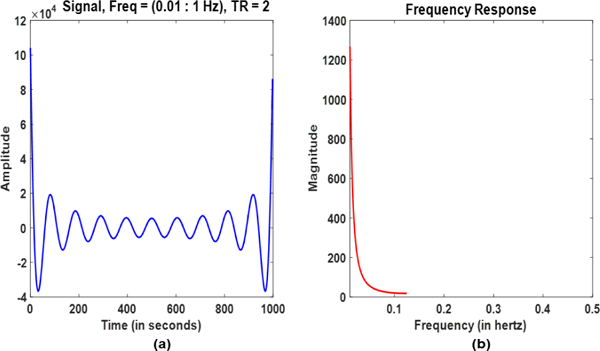
(a) Sum of sinusoids with increasing frequencies and decaying amplitudes. (b) Frequency spectrum of the signal.
The detail derivation of the above equation for the values of E, F, G, and H are available in the Supplementary file. Since the two signals are deterministic so their relationship is not dynamic. Consequently, the SWCov (SWC) is expected to be the same as stationary covariance (correlation) in every window regardless of the window size. However, it can be observed from (4) that the results are dependent on the size of the window (w) as discussed below.
-
1)Infinite Window Length: Stationary covariance over the entire signal length would be obtained from (4) when w →+∞ [6], and the value of the stationary covariance would be:
(5) -
2)
Finite Window Length: For window length (w) spurious fluctuations would be introduced from last four terms in (4). As a result, the covariance over the finite window w would approach the stationary covariance when these terms are zero (i.e., E, F, G, and H = 0) resulting in (Supplementary file for details):
It shows that all the frequencies can be expressed as multiples of the minimum frequency f1. Putting all the higher frequencies as multiples of lowest frequency f1 can have two possibilities (Supplementary file for details).
-
1)
Case 1: fj is an integer multiple of
In this case only the first term in (4) will be non-zero and the SWCov would approach the stationary covariance similar to the results of [6] and [5].
-
2)
Case 2: fj is an not an integer multiple of
This would result in last four terms of (4) to be zero only when w cancels out all multiples of f1 in arguments of all sin() functions (Supplementary file for details). In the absence of such a window length the SWCov would not be able to estimate the stationary covariance reliably.
From these observations we conclude that for deterministic signals comprising the sum of sinusoids the SWCov would be able to estimate the stationary (real) covariance for a window of length (or at its integer multiples) only when all the higher frequencies are integer multiples of fmin. Otherwise, the window length w has to cancel out the non-integer multiples of fmin for all sin() functions in (4).
The terms E, F, G, and H in (4) involve phase differences (θs) indicating that the spurious fluctuations introduced by the SWCov would be dependent on the phase differences, too.
B. Results
Results for the dependence of SWCov on frequencies, phases, and amplitudes of the correlating signals are given below.
-
1)
Frequency Dependence: Fig. 2. shows the plots when the deterministic correlating signals contain more than ninety frequency components that are integer multiples of the minimum frequency in (a) and not integer multiples in (b). Plots(c) and (d) are zoomed in version of the plots above them.
We plot the results for various window locations to evaluate if the SWCov reliably estimates stationary covariance for all window locations when as reported in [6]. In both of these cases the minimum frequency is at 0.01 Hz, phase differences are zero, and sinusoids have same amplitudes. It can be observed ((a) and (c)) that the SWCov reliably estimates the stationary covariance (black horizontal line) when the minimum window length is (vertical blackline) for all window locations. However, this is not the case when the frequencies are not integer multiple of fmin as shown in (b) and (d).
-
2)
Phase Dependence: Fig. 3. shows influence of non-zero phase difference on the results of the SWCov. The fmin is 0.01 Hz, all frequencies are integer multiple of fmin, and all sinusoids have same amplitudes. Fig. 3. contains plots for variable phase differences in (a) and constant one in (b). The SWCov results estimate the stationary covariance reliably in both cases, however, constant phase difference resulted in smoother SWCov time course as seen in (b).
-
3)
Amplitude Dependence: Fig. 4. shows influence of changing the amplitudes of the sinusoids. In (a) amplitudes are same and in (b) the amplitudes are changing as In both of these cases the minimum frequency is at 0.01 Hz, all phases are taken to be zero, and higher frequencies are integer multiples of fmin. It can be observed that the values of SWCov is different in both cases, however, the pattern of values is the same and it is estimating stationary covariance (black horizontal line) when .
-
4)
Minimum-Frequency Dependence: Fig. 5. shows the influence of different minimum frequencies in the correlating signals. The phase difference is zero here, amplitudes are constant, and the window is placed at the same location for all of these plots. However, the minimum bandpass cutoffs are different for each case (0.01, 0.02, 0.05, 0.06, and 0.08 Hz). These frequencies correspond to minimum window length (to estimate the stationary correlation) ranging from 12.5 to 100 seconds. Plots in (a) correspond to the minimum window length for each of above mentioned frequencies when both the correlating signals contain just the fmin sinusoid. In (b) the window lengths are same as in (a) but a frequency other than the minimum frequency (not necessarily an integer multiple of the minimum frequency) is added. It can be observed that in (a) the SWCov is estimating the stationary covariance (horizontal black line) accurately at the minimum window lengths (black vertical lines). However, it fails to do so in (b) if the higher frequency was not an integer multiple of the lower frequency. Hence, addition of just one frequency is influencing the estimation properties of the SWCov.
Fig. 2:
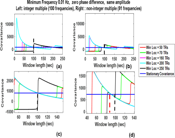
Sliding window covariance of deterministic signals with multiple frequency components for different window locations (Win Loc). (a) When all the higher frequencies are integer multiples of the minimum frequency and (b) when they are not integer multiples. (c) is zoomed in view of (a) and (d) which is zoomed in view of (b). In (d) the sliding window covariances are converging to stationary covariance for a window (vertical red line) other than the minimum window length (vertical black line).
Fig. 3:
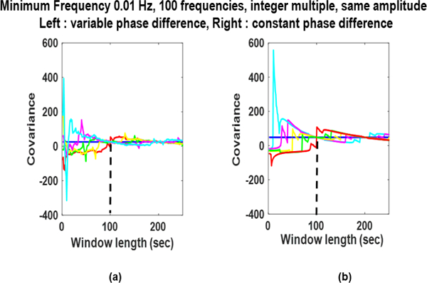
Sliding window covariance of deterministic signals with multiple frequencies and on-zero phase difference for different window locations. Phase difference is varibale in a) and is constant in (b).
Fig. 4:
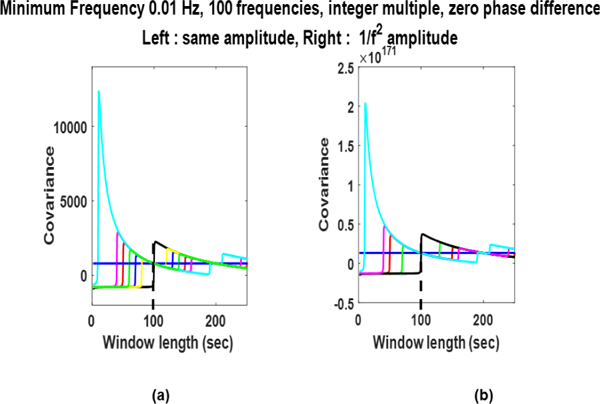
Sliding window covariance of deterministic signals with different amplitudes. In (a) amplitudes are same and in (b) the amplitudes are changing as .
Fig. 5:
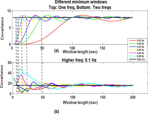
Sliding window covariance of deterministic signals with zero phase difference, and different minimum frequencies. The correlating signals have just fmin in (a) and have two frequencies in (b).
C. Sliding Window Correlation
The SWC is the SWCov normalized by the standard deviations and as shown in (1) over each window. To avoid further complexity we are not giving the details of these terms here. However, similar to the terms in SWCov, standard deviations would involve one term independent of window length and the rest would be dependent on the window length. They would normalize the stationary covariance for an infinite window and would influence the spurious fluctuations for finite windows similar to [6]. So, overall the SWC would follow the same pattern as sliding window covariance but the values would be normalized between −1 and 1. Hence, for finite windows, similar to the SWCov, the SWC would reliably estimate the stationary correlation (for windows which are an integer multiple of only if all the higher frequencies are an integer multiple of the fmin for sum of sinusoids.
iii. Modulated Signal (Dynamic Relationship)
The SWC is expected to capture the dynamics of the FC in the real rsfMRI signals. Until this point in our study we focus on exploring the inherent limitations of the SWC process itself by using deterministic signals. However, in next part of the study we investigate the efficiency of the SWC to capture the dynamics of the relationship between correlating signals. Similar to [6] and [5] we modulate one of our signals with low frequency sinusoids in order to introduce dynamics (non-stationarity) in their relationship. For this purpose, we multiply the signal yi with two modulating signals cos(2πf01iTR) and cos(2πf02)iTR, in which . In order to reduce the complex computations we are taking only two frequencies (and) for both xi and yi. We also assume the zero phase difference between the two signals. The modulated signal yi is given by:
| (6) |
From the above equation it is evident that the desired non-stationarity (dynamics) in the relationship between the two signals is introduced by two frequencies: f03 = f02 + f0i and f04 = f02 — f0i and SWCov (SWC) should be able to extract these frequencies only. Solving for covariance in Fourier domain (Supplementary file for details) we conclude that in the presence of dynamics (introduced by modulation of one signal) the higher frequency f2 needs to be above a certain multiple of the lower frequency . Otherwise, frequencies other than the desirable dynamics (comprising the frequency components f03 and f04) would be captured by SWCov (SWC).
A. Results
It can be observed from Fig. 6. that frequency components other than the desirable frequencies are retrieved when above mentioned condition in Section III is not met. These frequencies are introduced due to aliasing of frequencies when.
Fig. 6:
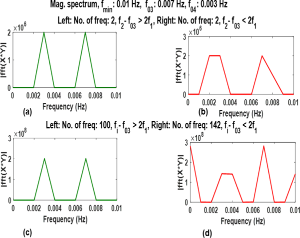
Plots of the SWC for signals with two frequency components when (a) f2 — f03 > 2f1 and (b) f2 — f03 < 2f1 and for 100 frequency components when (c) and (d) . Undesirable frequency components can be noticed in (b) and (d)
IV. Sliding Window Correlation for Real Data
Until this point this study was focused on exploring influence of various parameters on the SWC results for correlating sinusoids. However, real rsfMRI data is not expected to be composed of simple sinusoids (even though it can almost always be approximated by sum of sinusoids [35]). This section explores the dependence of the SWC results on different parameters of the correlating signals from real resting-state data.
A. Data and Preprocessing
We used rsfMRI scans of nine healthy human subjects (four females, ages: 21–57 years, downloaded from (http : //www.nitrc.org/prajects/fcon1000/). The scans were done on SIEMENS MAGNETOM TrioTim syngo MR B17 scanner. The scanning parameters were: TR = 645 ms, voxel size = 3mm isotropic, duration = 10 min, TE = 30 ms, slices = 40, multi-band accel. factor = 4, time points = 900. Initial 10 volumes of each scan were discarded to compensate for transient scanner instability. All preprocessing was done in statistical parametric mapping toolbox (SPM 12, http://www.fil.ion.ucl.ac.uk/spm/). Preprocessing included motion correction, coregisteration of the functional images with the anatomical image, segmentation, normalization, and smoothing. Default parameter values from SPM12 were used during preprocessing but smoothing was done using a Gaussian kernel of size 8 and for normalization a voxel size of 3×3×3 was chosen. The images were co-registered to the AAL atlas [36] using nearest neighbor interpolation without any warping. After preprocessing, four functional networks (Dorsal DMN, Ventral DMN, Visuospatial, and Sensorimotor) were extracted from gray matter regions using the masks from the Stanford’s functional imaging in neuropsychiatric disorders (FIND, http://findlab.stanford.edu/home.html) lab [37] for all subjects.
B. Network Time Series
In order to perform the SWC, we formed the time series of the four networks mentioned above (Subsection IV–A) by using the masks given in [37] for all nine subjects. Time series of each network was formed by taking the mean of all of its voxels’ intensities at every time point. Time series of each network for all the subjects were zscored and then concatenated. All the analysis reported in this study was done on the zscored concatenated time series for two of the four networks (Sensorimotor and Visuospatial) after band pass filtering them (0.01–0.1 Hz, FIR, order 80). However, similar results were obtained for the analysis with any two of the four networks. The filtered band of frequencies was 0.01–0.1 Hz unless otherwise specified.
C. Sliding Window Correlation and Frequency Response
We estimated the SWC and corresponding magnitude spectrum for six windows (50, 100, 150, 200, 250, and 300 TRs). In this case the minimum window length to avoid spurious fluctuations [5], [6] would be 100 seconds (155 TRs). We selected window sizes below (50 and 100 TRs), above (200, 250, and 300 TRs) and almost equal (150 TRs) to this size. Fig. 7. shows the results of the SWC in (a) and corresponding frequency responses in (b).
Fig. 7:
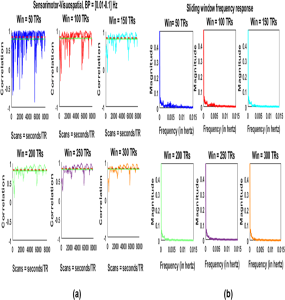
(a) Stationary correlation (red), mean sliding window correlation (green), and sliding window correlations for different windows. (b) Frequency spectrum of the results in (a).
Each plot in (a) also has stationary correlation value (in red) and mean of the SWC (in green). As expected the SWC time courses have higher frequencies for smaller windows (below 150 TRs) and lower for larger windows. Frequency spectrum plots in (b) have significant amount of power (magnitude) at the frequencies below fmin (0.01 Hz) which may be the result of dynamics (non-stationarity) in the FC as reported in [6]. However, the frequencies containing significant powers are dependent on the window length also since a sliding window acts as a low pass filter with cutoff at .
D. Dependence on Window Position
In [6] it was reported that the SWC would estimate the stationary correlation (for sinusoids) or mean of the SWC (for real resting-state data) for any window position provided that the size of window is larger than .
We explored this result for our data by changing the position of the window and the results are shown in Fig. 8. We placed the windows (a) at the start, (b) in the middle, and (c) at the end of the concatenated time series. The spurious fluctuations diminish with the increase in window size and SWC results converge very close to a value (mostly the mean of the SWC plotted in blue). However, the convergence is not at (black vertical lines) but at some other window size (green dashed vertical lines) always larger than. The exact size of this window is not evident but it falls within a range (between 200 and 250 TRs in Fig. 8).
Fig. 8:
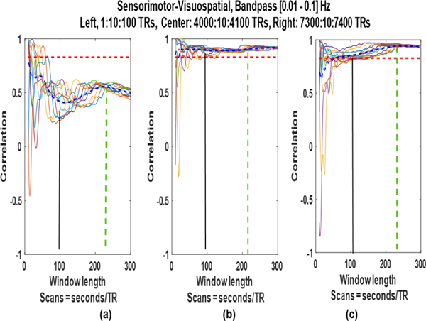
Sliding window correlation of the bandpass filtered (0.01–0.01 Hz) signals for three different sets of window positions.
The SWC results do not converge to stationary correlation (red horizontal lines) which shows that stationary correlation is not the true representative of the relationship between two time series for short time scale [22]. These results show that the spurious fluctuations arising from the SWC reduce significantly for larger windows () and exact size of this window is difficult to find. However, range of this window size can be estimated which may be used for dynamic FC analysis in the absence of some better method of estimating the best and maybe adaptive window size.
E. Dependence on Window Type
We also estimated the SWC using tapered windows (Hamming and Chebyshev) and the results are shown in Fig. 9. It can be seen that the tapered windows provide smoother results as expected, however, the change in window type does not change the convergence point of the SWC to.
Fig. 9:
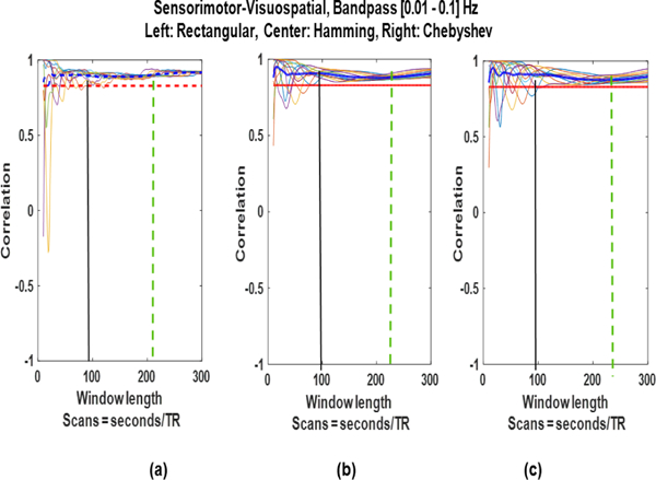
Sliding window correlation results for different window positions using (a) rectangular, (b) Hamming, and (c) Chebyshev windows.
F. Dependence on Filter Type
In order to compute the influence of filter type on the SWC results, we compared the results of bandpass (0.01–0.1 Hz) and highpass (0.01 Hz) filtered time series of the two networks. Fig. 10. shows the results of application of these two filters. It can be observed that in both cases the SWC converges to the same correlation values for windows larger than 100 seconds (155 TRs), however, inclusion of higher frequencies reduced the spurious fluctuations.
Fig. 10:
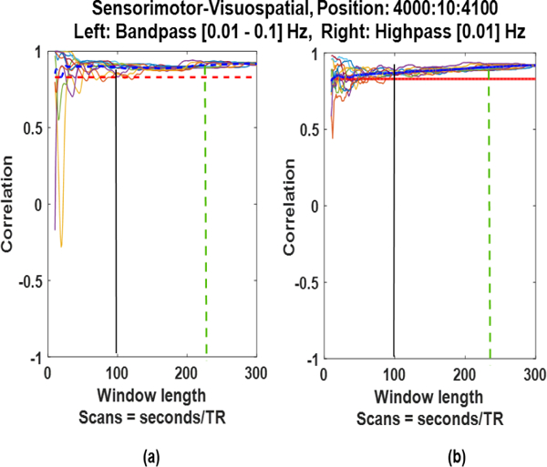
Sliding window correlation of the (a) bandpass filtered (0.01–0.1 Hz) and (b) highpass filtered (0.01 Hz) time series.
G. Dependence on Bandpass Cutoffs
We observed the influence of change in the bandpass cutoff by changing only the lower cutoff in Fig. 11. (a, bottom row) and only the higher cutoff in Fig. 11. (b, bottom row) from the cutoffs we used before (0.01–0.1 Hz, top row). We are taking the window positions that provided the best (fastest) convergence (in Section IV–F) to compare these results. Reducing the lower cutoff in ((a), bottom) moves minimum window length to avoid spurious fluctuations from 100 seconds (155 TRs) to 62.5 seconds (97 TRs). It can be observed that in this case the SWC convergence point changes with the change in frequency band. It shows that the frequency band of the correlating signals (and not the minimum frequency only) plays an important part in deciding the best window length.
Fig. 11:
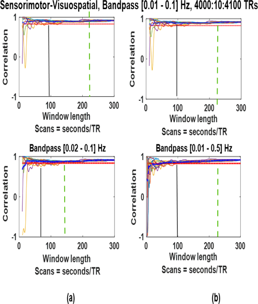
Changing the lower (a, bottom row) or upper (b, bottom row) cutoff of the frequency band influences the convergence of the sliding window correlation results.
H. Dependence on Network
We picked two different sets of networks (Sensorimotor, Visuospatial and Dorsal DMN, Ventral DMN) in order to see if the selection of network influences the SWC results. It can be seen from Fig. 12. that change in the network pair does
Fig. 12:
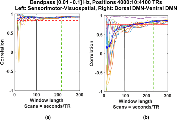
Sliding window correlation results changed based on the correlating networks.
I. Frequency Response Comparison
In [6] it was reported that dynamics (non-stationarities) of the FC are captured in the SWC results below fmin if. [5] reported that there has to be a specific relationship between higher and lower frequencies to achieve this result. We explored this result for real resting-state data under different conditions. Fig. 13. shows the results for (a) 150 TRs and (b) 200 TRs windows. First row is the frequency response (in dB) for bandpass (red) and highpass (green) filtered signals. It can be observed that in both the cases major power (magnitude) lies below 0.01 Hz (lower cutoff) which may be due to dynamics (non-stationary) in the FC. However, the power is greater for highpass which may be the result of some undesirable frequency components. Similar results were obtained for comparison of different frequency bands in second row and different network pairs in third row.
Fig. 13:
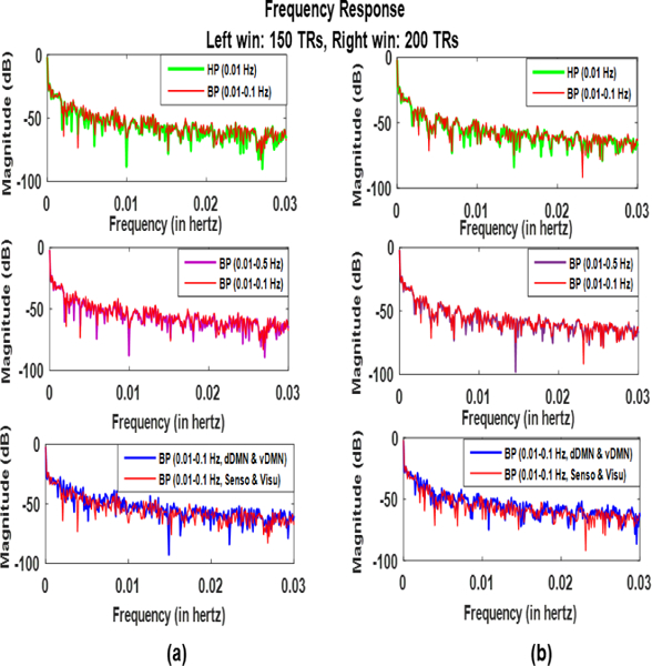
Comparison of frequency response of the SWC results under different conditions for (a) 150 TRs window and (b) 200 TRs window. Minimum cutoff for all cases is 0.01 Hz
J. Capturing Dynamics
In [6] it was reported that the SWC results would capture the non-stationarities of the correlating signals which are below fmin for a window of size ≥. However, our results show that increasing the size of the window would decrease the extracted non-stationarities since SWC acts as low pass filter with the cutoff equal to . Fig. 14. shows these cutoff
Fig. 14:
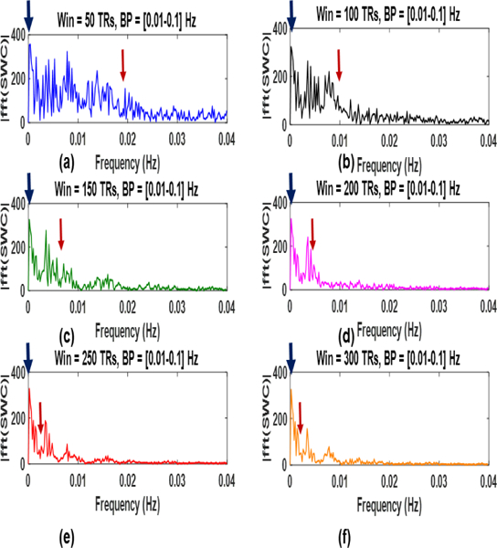
Magnitude spectrum for different windows having different low pass cutoffs (red arrows). The non-stationarities (dynamics) stabilize for best window range in (e) and (f).
This figure also shows the magnitude spectrum (blue arrows, after subtraction of mean SWC) that contributes the most and does not decay much with the increase in window length. Furthermore, the pattern of non-stationarities remains the same for the estimated best window range (between 200 and 250 TRs). This may be since the undesirable non-stationarities are rejected for these windows and the non-stationarities captured maybe the actual dynamics of the correlating signals.
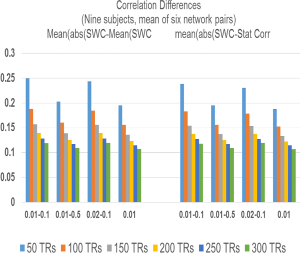
K. Means of all Network Pairs
To summarize our results we computed the means of results for all six network pairs of the four networks (Sensorimotor, Visuospatial, dorsal DMN, and ventral DMN). In order to observe how much the SWC differs from the stationary and mean SWC over the whole scan length, we computed the difference of the SWC for each window (50, 100, 150, 200, 250, and 300) and all frequency bands (0.01–0.1 Hz, 0.01–0.5 Hz, 0.02–0.1 Hz, and 0.1 Hz (highpass)) from stationary and mean SWC. We computed these differences for all network pairs and then computed means of absolute values of these differences. Fig. 15 . shows the plots of these means for all windows and frequency bands. It can be observed that the mean is decreasing as the size of the window increases which is an expected result. It can also be observed that for each window the means for the difference from mean SWC and from stationary correlations are almost the same. This shows that even though the SWC estimates differ from the stationary correlations for the duration of the window, capturing the short lived relationship of the correlating signals, but the mean of SWC results over the entire scan length approaches the stationary correlation value.
Fig. 15:
Correlation difference of the sliding window correlation from mean sliding window correlation (left) and from stationary correlation (rigth).
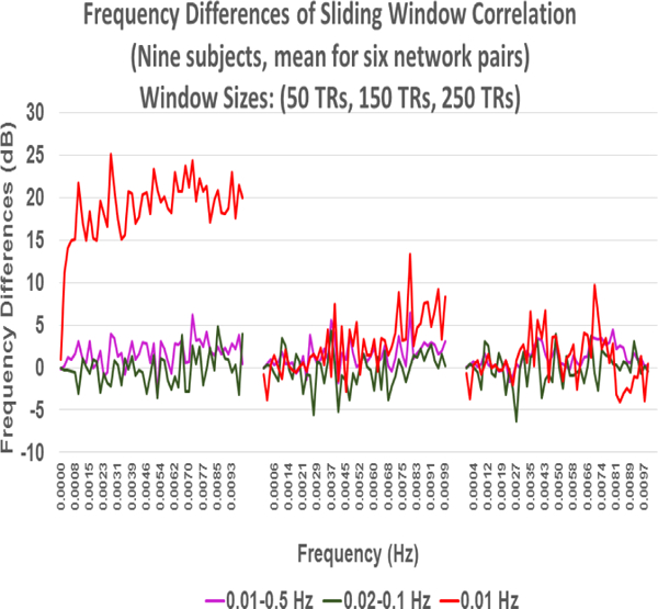
Fig. 16.showsthe difference (in dB) of the ampliltude spectrum of different frequency bands (0.01–0.5 Hz, 0.02–0.1 Hz, and 0.01 Hz (highpass)) from the most commoly used frequency band (0.01–0.1 Hz) for rsfMRI data. The plots are means of all six network pairs and three windows (50 TRs, 150 TRs, 250TRs) and the results are plotted from 0–0.01 Hz duration since this is the frequency band that should capture the non-stationarity of the correlating signals in the SWC results as mentioned in [6].
Fig. 16:
Difference of frequency spectrum of SWC results of bandpass (0.01–0.1 Hz) filtered signals from signals with other frequency components.
It can be seen that the amplitude differences for very low frequencies are small for larger windows (150 TRs, 250 TRs) for all frequency bands, however, they are not zeros for any case. These results indicate the changing the range of frequencies of the correlating signals would influence the frequency components of the resultant SWC time courses. In general higher power (amplitudes) are at the low frequencies (as shown in Fig. 13) but the power distribution changes with the change in frequencies. Furthermore, the difference is larger for highpass filtered data (red) for almost all the cases. From these results we can conclude that even though non-stationarity is captured in the SWC below the lower cutoff as reported in [6] but the exact frequency distribution changes with frequency components. In the absence of any ground truth it can not be established if these variations are because of some undesirable frequency components or are capturing the true non-stationarity in the relationship of the two signals.
L. Phase Randomization
We generated surrogate time series of correlating signals by phase randomization [38]. The frequency responses and autocorrelation of the time series remained the same after randomization of the phases. The results showed a lot of spurious fluctuations even after the window size increased. For frequency response also, we observed that the power at very low frequencies was almost 20–30 dB less than the power obtained for the same frequency band in original (nonrandomized) data. As a result, we conclude that the results observed in our study are not by chance.
v. Discussion
In this study we analyzed the impact of various parameters on SWC results. We started with deterministic signals followed by modulating one of the signals to introduce dynamics in their relationship. Similar to the results of [6] and [5] the SWC approached the stationary correlation when w (window length) ≥. However, the SWC estimated the exact stationary correlation value at this window (and at its integer multiples) only if the higher frequencies were integer multiples of the fmin. Furthermore, for dynamic relationship (in case of one modulated signal) we discovered that the SWC extracted undesirable frequency components if certain conditions were not met.
Similarly in real rsfMRI data also the SWC approached mean of the SWC when w (window length) ≥. This converging window length was different for different positions of the window but it was between some window range (e.g. between 200 and 250 TRs for Sensorimotor and Visuospatial networks with fmin = 0.01 Hz). This may be because the relationship between any two networks may change at unequal intervals at different times and same window can not capture variable length dynamics. Defining a range of these windows may help in approximating the best window size for the analysis. Changing the filter from bandpass to highpass or even changing the bandpass cutoffs resulted in modification of the results, however, convergence always occurred for larger windows. Moreover, even for the same frequency band the SWC results were different for different network pairs. Study of the frequency response of the SWC results showed that most of the power (magnitude) lies below the lower cutoff of the filter for larger windows as reported in [6] and [5]. This power from some undesirable dynamics (introduced as a result of frequency components of the correlating signals) in addition to the desired dynamics. The power at very low frequencies remain stable for all windows.
In this study we are not focusing on the influence of many source of variations (such as noise, motion), but only on the influence of the SWC itself. These results clearly identify the fact that the results of the SWC are dependent on many factors and the current methods of choosing a window size may be limiting the output of the method. Our study validates the results about the minimum window length to minimize the spurious fluctuations and frequency distribution of the SWC results in [6] and [5], however, it also shows that the SWC with one window length may not be able to capture the dynamics correctly. We may either define a range of window lengths or develop a better method of estimating the adaptive window length.
VI. Conclusion
For deterministic time series the SWC reliably estimated the stationary correlation when higher frequencies were integer multiple of the fmin. Furthermore, when the dynamics were introduced in the relationship of two signals, the SWC captured the modulating frequencies under specific conditions only. Similar results were observed for real rsfMRI data also and based on those results the following recommendations can be made for the choice of best window length:
-
1)
The SWC should be estimated by placing the window at various locations and changing its size from very small to very large.
-
2)
Range of window lengths providing the best estimate of the mean SWC should be noted.
-
3)
The window in this range should be able to capture the true dynamics (non-stationarity) of the FC reliably and this can be confirmed by plotting the frequency spectrum of the result for different window lengths.
-
4)
14 The non-stationarity captured can be used to study the dynamics of resting-state networks.
The SWC based studies may define a range of window sizes but this is still not the optimum way to capture FC dynamics. In future, studies may look into new ways of dynamic analysis of the FC. There are number of scenarios that can be explored for this purpose. One possibility can be to detect efficient window size by observing the peaks of cross correlation between the two correlating signals. The future work in this direction may also focus on the formation of some frequency dependent model by using some data driven method such as Hilbert-Huang Transform [39]. Another possibility can be to identify the change points of these networks adaptively by image processing of the rsfMRI scans [40]. Any two consecutive change points may represent the time of change in the network dynamics.
Supplementary Material
Acknowledgment
This research was supported by the Fulbright Scholarship Program. The authors would like to thank their lab members Anzar Abbas, Wen-Ju Pan, and Maysam Nezafati for sharing their views on different aspects of the study. The authors would also like to thank Dr. Aamer Iqbal Bhatti of Capital University of Science and Technology, Islamabad, Pakistan for sharing his ideas for the future work in this domain.
Biography

Dr. Sadia Shakil earned her BSc in Mathematics and Physics, and later her two masters’ degrees in Electronics and Computer Engineering from Pakistan. Afterwards, she won the Fulbright scholarship for her doctoral study in Electrical and Computer Engineering from Georgia Institute of Technology, Atlanta, USA in 2011. Currently she is working as Assistant Professor at the Institute of Space Technology, Islamabad, Pakistan. Dr. Shakil is recently awarded the Schumberger Foundation Faculty for the Future Fellowship and will proceed for Postdoc in Computational Connectomics shortly at the University of Toronto. Her research focus is on exploring the dynamics of the functional connectivity in the resting brain, with emphasis on development of new algorithms for this purpose.

Dr. Jacob Billings earned a BS in chemical (biomedical) engineering from The FAMU/FSU College of Engineering,Tallahassee,USA. He went on to earn a Ph.D. in Neuroscience from Emory University, Atlanta, USA, focusing on the intersection of neuroimaging and data science in the representation of spontaneous brain dynamics. Dr. Billings is currently interested in the relationship between human communications technologies and political networks.

Dr. Shella Keilholz obtained her BS in physics from the University of MissouriRolla (now Missouri University of Science and Technology). Her PhD in Engineering Physics at the University in Virginia focused on quantitative measurements of perfusion with arterial spin labeling MRI. After graduation, she went to the NIH as a postdoctoral researcher in Alan Koretskys lab to learn functional neuroimaging. She is currently an associate professor in the joint Emory /Georgia Tech Biomedical Engineering department. Her research seeks to elucidate the neurophysiological processes that underlie the BOLD signal and develop analytical techniques that leverage spatial and temporal information to separate contributions from different sources.

Dr. Chin-Hui Lee is a professor at School of Electrical and Computer Engineering, Georgia Institute of Technology. Before joining academia in 2001, he had 20 years of industrial experience ending in Bell Laboratories, Murray Hill, as a Distinguished Member of Technical Staff and Director of the Dialogue Systems Research Department. Dr. Lee is a Fellow of the IEEE and a Fellow of ISCA. He has published over 450 papers and 30 patents, with over 30,000 citations and an h-index of 70 on Google Scholar for his publications. He received numerous awards, including the Bell Labs President’s Gold Award in 1998. He won the SPS’s 2006 Technical Achievement Award for “Exceptional Contributions to the Field of Automatic Speech Recognition”. In 2012 he gave an ICASSP plenary talk on the future of speech recognition. In the same year he was awarded the ISCA Medal in scientific achievement for “pioneering and seminal contributions to the principles and practice of automatic speech and speaker recognition”.
Contributor Information
Sadia Shakil, School of Electrical and Computer Engineering, Georgia Institute of Technology, Atlanta.
Jacob C. Billings, Emory University, Graduate Division of Biological and Biomedical Sciences - Program in Neuroscience, Atlanta, USA
Shella D. Keilholz, School of Biomedical Engineering, Georgia Institute of Technology and Emory University School of Medicine, Atlanta, GA, 30332, USA..
Chin-Hui Lee, School of Electrical and Computer Engineering, Georgia Institute of Technology, Atlanta, GA, 30332 USA..
References
- [1].Sorg C et al. , “Selective changes of resting-state networks in individuals at risk for alzheimer’s disease,” Proc Natl Acad Sci, vol. 104, no. 47, pp. 18 760–5, 2007. [DOI] [PMC free article] [PubMed] [Google Scholar]
- [2].Rombouts S et al. , “Altered resting state networks in mild cognitive impairment and mild alzheimer’s disease: an fmri study.” Hum Brain Mapp, vol. 26, no. 4, pp. 231–9, 2005. [DOI] [PMC free article] [PubMed] [Google Scholar]
- [3].Keilholz S et al. , “Dynamic properties of functional connectivity in the rodent,” Brain Connectivity, vol. 3, no. 1, pp. 31–40, 2013. [DOI] [PMC free article] [PubMed] [Google Scholar]
- [4].Kiviniemi V et al. , “A sliding time-window ica reveals spatial variability of the default mode network in time,” Brain Connectivity, vol. 1, no. 4, pp. 339–47, 2011. [DOI] [PubMed] [Google Scholar]
- [5].Shakil S et al. , “On frequency dependencies of sliding window correlation,” in International Conference of Bioinformatics and Biomedicine IEEE, 2015. [Google Scholar]
- [6].Leonardi N and Van De Ville D, “On spurious and real fluctuations of dynamic functional connectivity during rest,” Neuroimage, vol. 104, no. 1, pp. 430–6, 2015. [DOI] [PubMed] [Google Scholar]
- [7].Shakil S et al. , “Evaluation of sliding window correlation performance for characterizing dynamic functional connectivity and brain states,” NeuroImage, vol. 133, pp. 111–28, 2016. [DOI] [PMC free article] [PubMed] [Google Scholar]
- [8].Schulz D and Huston J, “The sliding window correlation procedure for detecting hidden correlations: existence of behavioral subgroups illustrated with aged rats,” J Neurosci Methods, vol. 121, no. 2, pp. 129–37, 2002. [DOI] [PubMed] [Google Scholar]
- [9].Chang C and Glover G, “Time-frequency dynamics of resting-state brain connectivity measured with fmri,” Neuroimage, vol. 50, no. 1, pp. 81–98, 2010. [DOI] [PMC free article] [PubMed] [Google Scholar]
- [10].Handwerker D et al. , “Periodic changes in fmri connectivity,” Neuroimage, vol. 63, no. 3, pp. 1712–9, 2012. [DOI] [PMC free article] [PubMed] [Google Scholar]
- [11].Chang C et al. , “Eeg correlates of time-varying bold functional connectivity,” Neuroimage, vol. 15, no. 72, pp. 227–36, 2013. [DOI] [PMC free article] [PubMed] [Google Scholar]
- [12].Hutchison R et al. , “Dynamic functional connectivity: Promise, issues, and interpretations,” Neuroimage, vol. 80, pp. 360–78, 2013. [DOI] [PMC free article] [PubMed] [Google Scholar]
- [13].Thompson G et al. , “Short time windows of correlation between large scale functional brain networks predict vigilance intra-individually and inter-individually,” Hum Brain Mapping, vol. 34, no. 12, pp. 3280–98, 2013. [DOI] [PMC free article] [PubMed] [Google Scholar]
- [14].Wilson R et al. , “Influence of epoch length on measurement of dynamic functional connectivity in wakefulness and behavioural validation in sleep,” Neuroimage, vol. 112, pp. 169–79, 2015. [DOI] [PubMed] [Google Scholar]
- [15].Allen A et al. , “Tracking whole-brain connectivity dynamics in the resting state,” Cerebral Cortex, vol. 24, no. 3, pp. 663–76, 2014. [DOI] [PMC free article] [PubMed] [Google Scholar]
- [16].Smith S et al. , “Temporally-independent functional modes of spontaneous brain activity,” Proc Natl Acad Sci, vol. 109, no. 8, pp. 3131–36, 2012. [DOI] [PMC free article] [PubMed] [Google Scholar]
- [17].Sakoglu U et al. , “A method for evaluating dynamic functional network connectivity and task-modulation: application to schizophrenia,” MAGMA, vol. 23, pp. 351–66, 2010. [DOI] [PMC free article] [PubMed] [Google Scholar]
- [18].Smith R et al. , “Wavelet-based regularity analysis reveals recurrent spatiotemporal behavior in resting-state fmri,” Hum Brain Mapp, vol. 36, no. 9, pp. 3603–20, 2015. [DOI] [PMC free article] [PubMed] [Google Scholar]
- [19].Yaesoubi M et al. , “Dynamic coherence analysis of resting fmri data to jointly capture state-based phase, frequency, and time-domain information,” Neuroimage, vol. 120, pp. 133–142, 2015. [DOI] [PMC free article] [PubMed] [Google Scholar]
- [20].Shine J et al. , “Estimation of dynamic functional connectivity using multiplicative analytical coupling,” Neuroimage, vol. 122, pp. 399–407, 2015. [DOI] [PubMed] [Google Scholar]
- [21].Lindquist M et al. , “Evaluating dynamic bivariate correlations in resting-state fmri: a comparison study and a new approach,” Neuroimage, vol. 101, pp. 531–46, 2014. [DOI] [PMC free article] [PubMed] [Google Scholar]
- [22].Rashid B et al. , “Classification of schizophrenia and bipolar patients using static and dynamic resting-state fmri brain connectivity,” Neuroimage, vol. 134, pp. 645–57, 2016. [DOI] [PMC free article] [PubMed] [Google Scholar]
- [23].Chang C et al. , “Tracking brain arousal fluctuations with fmri,” Proc Natl Acad Sci, vol. 113, no. 16, pp. 4518–23, 2016. [DOI] [PMC free article] [PubMed] [Google Scholar]
- [24].Hansen E et al. , “Functional connectivity dynamics: Modeling the switching behavior of the resting state,” Neuroimage, vol. 105, p. 525535, 2015. [DOI] [PubMed] [Google Scholar]
- [25].Shi Z et al. , “Realistic models of apparent dynamic changes in restingstate connectivity in somatosensory cortex,” Hum Brain Mapp, vol. 37, p. 38973910, 2016. [DOI] [PMC free article] [PubMed] [Google Scholar]
- [26].Raatikainen V et al. , “Combined spatiotemporal ica (stica) for continuous and dynamic lag structure analysis of mreg data,” Neuroimage, vol. 148, pp. 352–68, 2017. [DOI] [PubMed] [Google Scholar]
- [27].Deng L et al. , “Characterizing dynamic local functional connectivity in the human brain,” Scientific Report, 2016. [DOI] [PMC free article] [PubMed] [Google Scholar]
- [28].Dixon M et al. , “Interactions between the default network and dorsal attention network vary across default subsystems, time, and cognitive states,” Neuroimage, vol. 147, p. 632649, 2017. [DOI] [PubMed] [Google Scholar]
- [29].Trapp C et al. , “On the detection of high frequency correlations in resting state fmri,” Neuroimage, 2017. [DOI] [PMC free article] [PubMed] [Google Scholar]
- [30].Ma Y et al. , “Dynamic connectivity patterns in conscious and unconscious brain,” Brain Connectivity, vol. 7, no. 1, 2017. [DOI] [PMC free article] [PubMed] [Google Scholar]
- [31].Laughlin R et al. , “Correlative gene expression to protective seroconversion in rift valley fever vaccinates,” PLOS ONE, 2016. [DOI] [PMC free article] [PubMed] [Google Scholar]
- [32].Du W et al. , “Edge detection in potential filed using the correlation coefficients between the average and standard deviation of vertical derivatives,” Journal of Applied Geophysics, 2017. [Google Scholar]
- [33].Kafashan M et al. , “Sevoflurane alters spatiotemporal functional connectivity motifs that link resting-state networks during wakefulness,” Front. Neural Circuits, vol. 147, p. 632649, 2016. [DOI] [PMC free article] [PubMed] [Google Scholar]
- [34].Hindriks R et al. , “Can sliding-window correlations reveal dynamic functional connectivity in resting-state fmri?” Neuroimage, vol. 127, pp. 242–256, 2016. [DOI] [PMC free article] [PubMed] [Google Scholar]
- [35].Weeks M, Digital Signal Processing Using MATLAB Wavelets. Jones and Bartell, 2011. [Google Scholar]
- [36].Tzourio-Mazoyer N et al. , “Automated anatomical labeling of activations in spm using a macroscopic anatomical parcellation of the mni mri single-subject brain,” Magn Reson Med, vol. 15, no. 1, pp. 273–89, 2002. [DOI] [PubMed] [Google Scholar]
- [37].Shirer W et al. , “Decoding subject-driven cognitive states with whole-brain connectivity patterns,” Cereb Cortex, vol. 22, no. 1, pp. 158–65, 2012. [DOI] [PMC free article] [PubMed] [Google Scholar]
- [38].Prichard D and Theiler J, “Generating surrogate data for time series with several simultaneously measured variables,” Phys. Rev. Lett, vol. 73, no. 7, 1994. [DOI] [PubMed] [Google Scholar]
- [39].Norden E and Wu Z, “A review on hilbert-huang transform: Method and its applications to geophysical studies,” Rev. Geophys, 2008. [Google Scholar]
- [40].Shakil S et al. , “Adaptive change point detection of dynamic functional connectivity networks,” in 38th Annual International Conference of the IEEE Engineering in Medicine and Biology Society (EMBC) IEEE, 2016. [DOI] [PMC free article] [PubMed] [Google Scholar]
Associated Data
This section collects any data citations, data availability statements, or supplementary materials included in this article.