The effect of automated landmark identification on morphometric analyses

Abstract

Morphometric analysis of anatomical landmarks allows researchers to identify specific morphological differences between natural populations or experimental groups, but manually identifying landmarks is time‐consuming. We compare manually and automatically generated adult mouse skull landmarks and subsequent morphometric analyses to elucidate how switching from manual to automated landmarking will impact morphometric analysis results for large mouse (Mus musculus) samples (n = 1205) that represent a wide range of ‘normal’ phenotypic variation (62 genotypes). Other studies have suggested that the use of automated landmarking methods is feasible, but this study is the first to compare the utility of current automated approaches to manual landmarking for a large dataset that allows the quantification of intra‐ and inter‐strain variation. With this unique sample, we investigated how switching to a non‐linear image registration‐based automated landmarking method impacts estimated differences in genotype mean shape and shape variance‐covariance structure. In addition, we tested whether an initial registration of specimen images to genotype‐specific averages improves automatic landmark identification accuracy. Our results indicated that automated landmark placement was significantly different than manual landmark placement but that estimated skull shape covariation was correlated across methods. The addition of a preliminary genotype‐specific registration step as part of a two‐level procedure did not substantially improve on the accuracy of one‐level automatic landmark placement. The landmarks with the lowest automatic landmark accuracy are found in locations with poor image registration alignment. The most serious outliers within morphometric analysis of automated landmarks displayed instances of stochastic image registration error that are likely representative of errors common when applying image registration methods to micro‐computed tomography datasets that were initially collected with manual landmarking in mind. Additional efforts during specimen preparation and image acquisition can help reduce the number of registration errors and improve registration results. A reduction in skull shape variance estimates were noted for automated landmarking methods compared with manual landmarking. This partially reflects an underestimation of more extreme genotype shapes and loss of biological signal, but largely represents the fact that automated methods do not suffer from intra‐observer landmarking error. For appropriate samples and research questions, our image registration‐based automated landmarking method can eliminate the time required for manual landmarking and have a similar power to identify shape differences between inbred mouse genotypes.

Introduction

Three‐dimensional (3D) or volumetric imaging is being increasingly used to study anatomical variation in both comparative and biomedical contexts (Hallgrímsson & Jones, 2009; Lerch et al. 2011; Deans et al. 2012; Wong et al. 2012; Norris et al. 2013; Hallgrimsson et al. 2015; Nieman et al. 2018). Increasingly, such imaging datasets are integrated with genomic, molecular or ecological data to better elucidate the multivariate factors that determine complex phenotypes. Successfully identifying subtle morphological effects of specific factors requires a large number of samples across which phenotypic measurements are directly comparable (Benedikt et al. 2009). Multivariate statistical approaches to quantifying phenotype commonly rely on the analysis of 3D anatomical landmarks. Anatomical landmarks are points on a structure representing anatomical or biological features of interest that can be identified consistently and precisely. A well‐chosen set of anatomical landmarks represents the form of a specimen and allows for morphometric comparisons. However, manual landmark identification can be time‐consuming and datasets collected by different observers may not be directly comparable. The use of atlas‐based image registration techniques that accurately identify homologous anatomical landmarks across a large dataset may save time and algorithmically standardize landmark placement within and across studies (Bromiley et al. 2014; Young & Maga, 2015; Maga et al. 2017). The results of such methods might also serve as the basis for the sort of high‐throughput and consistent datasets required for ‘phenomic’ analysis (Houle et al. 2010). However, a better understanding of how well automated landmarks represent biological shape and sample‐wide shape variation is necessary before embracing image registration‐based automated landmarking methods.

It is critical that each anatomical landmark represents a biologically or geometrically homologous feature on all specimens, because any measurement derived from a landmark should be directly comparable across a sample (Bookstein, 1991; Lele & Richtsmeier, 2001; Zelditch et al. 2012). Bookstein's (1991) influential landmark types are defined by the degree of local anatomical homology and it is widely stressed that landmarks with better homology should be preferred. Morphometric measures of interest include linear distances and angles measured between landmarks or variation in landmark coordinates after scaling and superimposition of all specimens into a single coordinate system (e.g. Procrustes superimposition; Gower, 1975). One popular form of morphometrics, ‘geometric morphometrics’, is the statistical analysis of shape using Cartesian landmark coordinates after Procrustes superimposition.

A single expert observer typically identifies landmarks on all specimens being analyzed within a single study to avoid inevitable inter‐observer error. An expert observer should be aware of the morphological variation across their sample and have experience with their landmark collection protocol. For large datasets collected over months or years, manual landmark collection is time‐consuming, requires an observer to maintain consistent landmark placement and can be very dull. Semi‐automated landmarking approaches have been implemented (including in landmark editor and morpho; Schlager, 2017) roughly to place a standard set of homologous landmarks so that an expert observer can more efficiently move them to their precise homologous locations. However, semi‐landmarking methods may not always substantially improve landmarking efficiency given that users are required to open all images and look at all landmarks. And because they rely on expert observer assessment, inter‐observer variation still limits consistency across datasets.

Fully automated landmarking methods based on 3D surface curvature (Subburaj et al. 2009; Wilamowska et al. 2012; Guo et al. 2013; Li et al. 2017) and image volume registrations (Ólafsdóttir et al. 2007; Chakravarty et al. 2011; Bromiley et al. 2014; Young & Maga, 2015; Maga et al. 2017) have been suggested to replace manual landmarking. Ideally, automated landmarking methods would produce high‐quality algorithmically standardized landmark datasets in much less time than a manual observer. Registration of brain magnetic resonance images (MRIs) to atlases is a common basis for the segmentation of brain into subregions and the quantification of morphological differences between experimental groups (Talairach & Tournoux, 1988; Mazziotta et al. 1995; Kovačević et al. 2004; Lerch et al. 2011). We tested the use of similar volumetric registration methods to generate anatomical landmark datasets automatically.

Alternate 3D surface‐based registration methods use dense clusters of pseudolandmarks, quasi‐landmarks or surface vertices to quantify bone (Boyer et al. 2015; Pomidor et al. 2016) and facial morphology (Claes et al. 2011, 2018). Within a study, each measured pseudolandmark position displays general topological correspondence across samples. This type of correspondence is different from, although analogous to, anatomical landmark homology. Although very promising, the impact of these methods on conclusions drawn from estimates of morphological shape variance and covariance (as compared with conclusions drawn from manual landmark‐based estimates) remain largely unreported. Because these methods also rely on 3D registration, they are likely to suffer from similar issues and biases as other surface or volume registration‐based landmark placement techniques, including those explored in our analysis.

We adapted nonlinear volumetric registration methods developed originally for the automated segmentation of brain region volumes from MRI images in order automatically to identify anatomical landmark positions on mouse skulls from computed tomography scans. Representative images with reference annotations called atlases serve as the basis for comparison of automated landmark placement within all specimen images. Image registration is the alignment of images that represent the same anatomical features. Affine image registration utilizes the same geometric transformations of translation, rotation and scaling that underlie Procrustes superimposition as well as shearing transformations. Non‐linear registration methods produce more precise local alignments consisting of a deformation vector for every voxel in a 3D image.

The atlases produced in our analysis are the average of successfully aligned images upon which reference landmarks are placed. These reference landmarks can be back‐propagated onto the original specimen images using the inverse of the transformations required to align the original specimen images together. Features that are present similarly within all specimens appear sharp within these atlas images, whereas features that are more stochastic between specimens appear blurrier (Kovačević et al. 2004; Zamyadi et al. 2010; Wong et al. 2012). When there is a high degree of anatomical variation across a sample, the use of multiple atlases that represent subgroups may improve final image alignments and the accuracy of phenotype quantification. For example, independent averages of C57BL/6J and 129S1/SvImJ embryonic day (E)15.5 mice were used during a comparison of genotype organ volumes (Zamyadi et al. 2010). Similarly, the quantification of major ontogenetic changes in whole body anatomy across a sample of E11.5–E14.0 mice required the use of separate averages at half‐day intervals (Wong et al. 2015).

Recent analyses have shown that image registration‐based automatic landmarks largely replicate manually identified anatomical landmark position and successfully capture mean differences in skull shape between mouse groups (Bromiley et al. 2014; Young & Maga, 2015; Maga et al. 2017). However, each of these studies was completed on a small number of genotypes or specimens per genotype. We use a large existing dataset of micro‐computed tomography (μCT) images of adult mouse skulls (n = 1205) to better understand how image registration‐based automated landmarks differ from manual landmarks and how this impacts subsequent morphometric analysis. Our sample includes approximately 20 specimens from each of the eight Collaborative Cross founder strains and their reciprocal F1 crosses, which represent much of the phenotypic variation found within common and wild‐derived laboratory mice (Churchill et al. 2004; Chesler et al. 2008; Consortium, 2012). This type of large intra‐species dataset is exactly the kind of dataset for which automated landmarking will be the most valuable, because of the large number of specimens, known genotypes, and the broad range of ‘normal’ morphology in the sample. The use of large samples of Collaborative Cross mice (or the derived Diversity Outbred mice) allow for the identification of genetic factors that underlie normal phenotypic variation in mice and other mammals, including humans. Although other studies have explored the feasibility of various automated landmarking methods, this is the first to compare the utility of current automated approaches to manual landmarking for a large dataset that allows the quantification of intra‐ and inter‐strain variation. Determining the effect of switching from manual to automated anatomical landmark placement in this dataset is critical for researchers considering the application of similar methods in other large intra‐species datasets.

Although there is always some intra‐observer error for manually placed landmarks, the mean location of anatomical landmarks identified by an expert observer should represent the accurate position of that landmark. Therefore, the mean distance between manual and automatically identified landmark positions serves as the basis for estimating error in automated landmarking. We hypothesized that landmarks found within regions of the μCT images that demonstrate poor local alignment would have higher automated landmark placement error.

Due to the relatively high level of ‘normal’ phenotypic variation within our sample, we completed two separate automated registration procedures to determine whether initial genotype‐specific alignment would improve the quality of final μCT image alignment and landmark estimation (Fig. 1). A one‐level procedure was completed to align all specimen images to the overall sample average (Kovačević et al. 2004). A two‐level procedure may improve the quality of final alignments by first aligning all specimens of a single genotype to their genotype average, and secondarily aligning the images to the overall sample average (Friedel et al. 2014). We hypothesized that the two‐level registration would improve local alignments across the skull, leading to more accurate automated landmarking.

Figure 1.

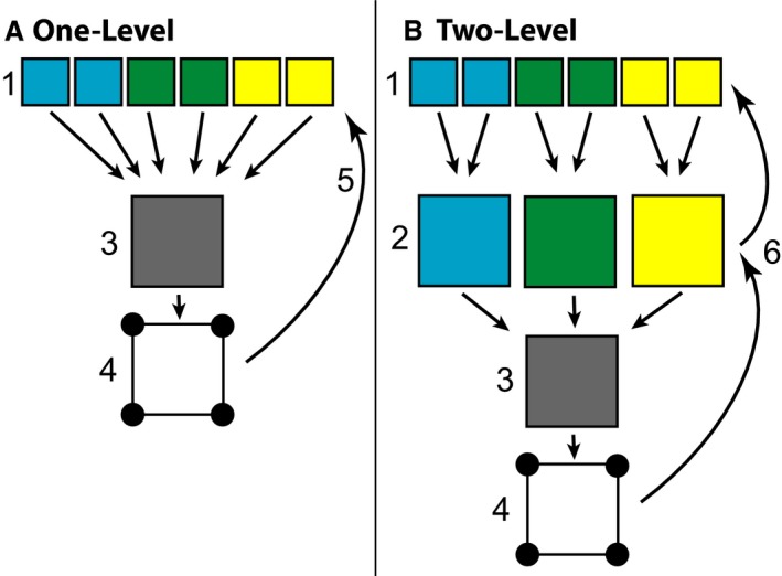
Image Registration Flowchart – Simplified schematic of the (A) one‐level and (B) two‐level registration methods. During one‐level registration, CT images of specimens from multiple genotypes (1) are registered directly to an averaged image of all genotypes (3). Landmarks collected on that average (4) are back‐propagated onto the original images using the inverse of a specimen's registration transformation (5). During two‐level registration, specimens (1) are registered to a genotype average image (2) before that average is registered to the average of all genotypes (3). Landmarks are back‐propagated using the inverse of the combined specimen and genotype average registration transformations (6).

A landmark‐based geometric morphometrics analysis was performed to determine whether overall patterns of mean shape variation between the genotypes of our sample were similarly identified by manually and automatically located landmarks. In addition, our large sample size allowed us to quantify whether differences in shape variance were also replicated by the automatically produced landmarks. A reduction in measured shape variance would reduce statistical power to determine differences in mean shape among groups if less biological variation is captured by automated landmarking. Alternatively, if the reduction in variance compared with manual landmarking is due to reduced measurement error, statistical power to detect differences in mean shape should be increased. Effects on shape variance may also bias studies of canalization or integration (Hallgrimsson et al. 2018).

Here, we test the landmark identification accuracy of two μCT image registration pipelines and whether automating landmark placement modifies the results of skull shape geometric morphometric analyses for a large mouse sample. We test the hypotheses that automated landmarking captures the same biological variation as manual landmarking, and that it preserves statistical power for comparisons of shape among groups. Further, we determine whether using a one‐ or two‐level registration strategy improves the ability to identify biological differences among genotypes. Our results are valuable to a wide range of researchers who are interested in the possibility of automating phenotypic measurements collected from large sets of variable μCT images.

Methods

Images and manual landmarks

Our sample of 1205 mouse skull μCT images were previously acquired and manually landmarked for analysis of the genetic structure of ‘normal’ laboratory mouse skull morphology (Percival et al. 2016; Pavličev et al. 2017). There are approximately 20 samples for each of eight inbred founder strains of the Collaborative Cross (Churchill et al. 2004; Chesler et al. 2008; Collaborative Cross Consortium, 2012) and 54 (of 56 possible) F1 crosses (Tables 1 and 2). This sample size is near the minimum required to identify consistently the mean differences in craniofacial morphology and differences in phenotypic variance between closely related strains (see Results for a power analysis). Each cross is identified by two letters, the first being the maternal founder strain and the second the paternal founder strain (Consortium, 2012). For example, BB is a C57BL/6J founder and BC is a C57BL/6J (dam) × 129S1/SvlmJ (sire) F1 cross. Because all founder strains are inbred, specimens within each founder strain and F1 cross are isogenic. Strain identity is referred to as specimen genotype throughout the analysis.

Table 1.

Definitions of CC founder strains, including letters used to identify them in the text, JAX strain abbreviations, and strain origin (Beck et al. 2000)

Letter	Strain ID	Strain origin
A	A/J	Lab Inbred (Castle's Mice)
B	C57BL/6J	Lab Inbred (C57 Related)
C	129S1/SvlmJ	Lab Inbred (Castle's Mice)
D	NOD/ShiLtJ	Lab Inbred (Swiss Mice)
E	NZO/HlLtJ	Lab Inbred (Castle's Mice/New Zealand)
F	CAST/EiJ	Wild Derived Inbred (Thailand)
G	PWK/PhJ	Wild Derived Inbred (Prague)
H	WSB/EiJ	Wild Derived Inbred (MD, USA)

Table 2.

Sample sizes for all crosses in our analysis

Maternal strain	Paternal strain
	A	B	C	D	E	F	G	H
A	18	18	19	20	19	20	20	20
B	20	19	19	18	19	20	16	18
C	21	17	19	17	18	19	24	22
D	19	21	19	13	22	24	21	17
E	19	18	22	20	17	0	0	19
F	20	26	19	17	21	18	22	18
G	19	21	20	17	19	18	18	18
H	19	19	20	20	19	28	20	18

Founder crosses are shown along the diagonal in bold, missing crosses are shown with gray background. Strains are identified by letters defined in Table 1.

These mice were bred as part of the Collaborative Cross breeding project at the University of North Carolina under the approval of the University of North Carolina Animal Care and Use Committee. These mice were housed at UNC for 8–12 weeks with standard chow and housing. Their secondary use to understand the genetics of craniofacial morphology illustrates the value of sharing animal specimens across independent research projects to reduce effectively the number of animals being bred. The μCT images were obtained in the 3D Morphometrics Centre at the University of Calgary with a Scanco vivaCT40 scanner (Scanco Medical, Brüttisellen, Switzerland) at 0.035–0.038 mm voxel dimensions at 55 kV and 72–145 μA. The 3D coordinates of 68 adult landmarks (Fig. 2), collected by a single expert observer from minimum threshold‐defined bone surfaces within ANALYZE 3D (www.mayo.edu/bir/), represent the manually identified landmarks in our analysis. A second manual landmarking trial was completed more than 4 years after the first trial by the same observer on a representative subset of 100 specimens to quantify intra‐observer landmark placement error.

Figure 2.

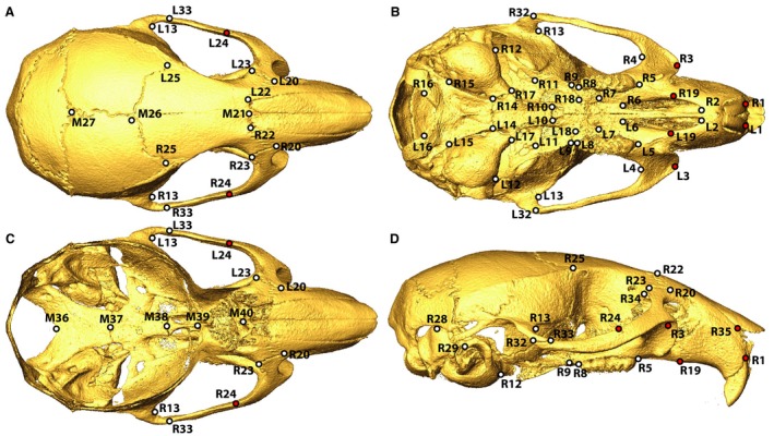
Skull Landmarks – Identification of landmarks used in morphometric analysis from (A) superior, (B) inferior, (C) interior (superior with calotte removed) and (D) lateral views. Red landmark centers identify the landmarks that were removed from the Procrustes superimposition‐based landmark comparisons because of high automated landmarking error (*in Table 2).

Image registration and automated landmarking

All μCT images were registered to an iteratively defined image average using Medical Imaging NetCDF (MINC) tools and the Pydpiper image registration toolkit (Friedel et al. 2014). All images were downsampled to 0.045‐mm voxel dimensions to reduce active memory usage, then affine‐transformed to a standard orientation and scale (7‐parameter alignment) based on manually collected landmarks. An initialization was required because the μCT images were not always collected in a standard orientation. While manual landmarks were used to orient specimens in preparation for automated registration, this initial affine registration does not create a bias in automated registration results (Wong et al. 2012). Improved standardization of specimen‐mounting during CT scanning should remove the need for manual landmarks entirely. With existing unaligned image datasets, incorporating a brute force alignment initialization step might also serve this purpose.

After initializing the alignment of μCT images, two separate registration strategies were used independently. The one‐level method involved iteratively registering all specimens to a single consensus image that represents all genotypes (Kovačević et al. 2004). The two‐level method involves first registering specimens to genotype‐specific consensus images, then registering the genotype‐specific aligned images to an overall consensus image that represents all genotypes (Friedel et al. 2014) (Fig. 1). The two‐level registration pipeline was completed on SciNet (Loken et al. 2010) and the one‐level was completed on the High Performance Computing Facility at the Hospital for Sick Children. Approximately 10 CPU hours were required per specimen for the two‐level registration procedure (total 500 CPU days), and marginally less time was required for the one‐level procedure.

Within each registration level, a randomly chosen subset of 25 of the possible pairwise 12‐parameter affine registrations from each image were computed. The average of all completed transformations for a specimen was calculated and the residual transforms applied to the respective image. An average intensity image was then calculated from the transformed images of all specimens. After 12‐parameter alignment, a two‐stage ANTS (Avants et al. 2009, 2011) non‐linear alignment procedure was performed in which each resulting image was registered towards the 12‐parameter average, and then subsequently towards the average of the first non‐linear stage. The non‐linear stages are meant to further improve local alignments across the images. Further details on specific alignment commands and parameters used can be found in the Supporting Information. A separate final atlas of all registered specimens was produced from both the one‐level and two‐level registration procedures (Fig. 3).

Figure 3.

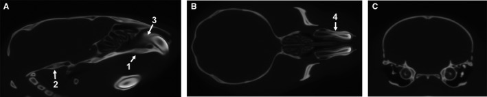
One‐level registration average image – Representative (A) sagittal, (B) transverse and (C) coronal slices through the final average image generated after affine and non‐linear registration procedures of the one‐level registration pipeline. Identifying which regions might not be well registered based on whether nearby anatomical features are sharp or blurry is more effective when scrolling through the slices of the 3D atlas images. However, we identify (1) the relatively blurry premaxilla‐maxillary suture area and (2) the relatively sharp spheno‐occipital synchondrosis to illustrate what a poorly registered and well registered suture area might look like. Also note (3) the relatively blurry posterior edge of the upper incisor compared with the (4) clear lateral edges of the incisor within the facial bones.

Our expert observer identified all anatomical landmarks (Fig. 2) on the final one‐level and two‐level atlases during a single landmarking session to minimize any differences in reference landmark placement between them. Minimizing these differences is critical because any differences between reference landmarks on different atlases would be propagated to registered specimens during the automated landmark placement process. Reference landmark coordinates on both atlases were inverse‐transformed to every original μCT image using a combination of existing commands to concatenate (xfmconcat) and invert (xfminvert) transformations within MINC Tools (see Supporting Information for more details on our pipeline). The resulting one‐level and two‐level landmark coordinates (automated landmarks) were compared with the manual landmark coordinates to determine how well the automated landmarking method reproduces manual landmark placement (Appendix S1).

Comparison of landmarking methods

Linear distances between manual landmark positions of each specimen with two manual landmark trials provides an estimate of intra‐observer manual landmarking error. This error is likely to be higher than what is expected for most landmark‐based studies during which landmarks are collected over a much shorter period of time than 4 years. Linear distances between manual trial one and the one‐level or two‐level automated landmark positions represent a combination of error in the automated method replicating manual landmark position and differences in manual landmark placement between an automated method's atlas image and specimen specific images. Subtracting the mean manual landmark intra‐observer error from the linear distance between manual and automated landmark positions provides a conservative estimate of the error with which our automated landmarking methods identify a given anatomical landmark.

Procrustes superimposition was completed on a dataset that includes manual, one‐level and two‐level landmarks for each specimen to quantify how the landmarking method impacts analyses of skull shape. Landmarks L/R1, L/R3, L/R19, L/R24 and L/R35 were removed from the dataset prior to superimposition because of their relatively high automated landmarking error. A Procrustes anova analysis with the landmarking method (manual, one‐level or two‐level) nested within specimen identifier was completed with geomorph (Adams et al. 2016) in R (R Developmental Core Team, 2008) to estimate the proportion of total landmark coordinate variance associated with inter‐specimen variation and the proportion associated with the landmark identification method (Kohn & Cheverud, 1992; Aldridge et al. 2005). A principal component analysis (PCA) of landmarks collected for the same dataset of all specimens using all methods was completed to provide a visualization of major axes of skull shape covariation (i.e. the first several principal components (PCs)).

Genotype‐specific Procrustes shape variances were estimated separately for each measurement method and compared to determine how landmark automation influences estimates of shape variation. A Kendall's rank correlation test was performed to determine whether genotypes show a similar order of relative Procrustes shape variance between manual and automated methods. To determine whether the three landmarking methods capture the same biological patterns, we compared the landmark variance‐covariance matrices across the three methods using both the matrix correlation with Mantel's test (Mantel, 1967) and random skewers (Marroig & Cheverud, 2001). We used both methods because Rohlf (2017) recently showed that random skewers are influenced by both the scale (eigenvalues) of variation and its direction. We performed this analysis on both the individual level Procrustes coordinates and on the genotype mean coordinates. Use of genotype means allows a comparison of genetic covariance structures that will be less influenced by random manual measurement error.

The results of separate PCAs of specimen Procrustes coordinates completed for each method were compared to identify similarities in major axes of skull shape covariation between the results of manual and automated landmarking methods. This included comparisons of eigenvalues and correlations of PC scores for the first several PCs. A similar analysis where PCs were calculated from genotype‐specific mean shapes rather than all specimen coordinates is included with the Supporting Information. These analyses were completed primarily with geomorph functions in R.

Procrustes distances among genotypes were compared across methods to determine whether the magnitude of genotype differences is similarly identified with automated and manual methods. The mean shape for each genotype (mean Procrustes coordinates) was computed for each method (manual, one‐level, two‐level). Pairwise Procrustes distances between genotype means were compared across methods. An anova of these distances was completed to test for differences in distance magnitudes between methods. Regressions were used to compare inter‐genotype distances across methods.

A Procrustes anova with genotype, landmarking method and their interaction was completed to determine whether there is a genotype‐specific bias in automated landmark placement. We tested the theory that genotypes further from the mean shape of all specimens will have larger errors in automated landmark placement. This was done by testing for a correlation of (1) the distance between manual genotype mean shape and the manual grand mean shape and (2) the distance between manual genotype mean shape and one‐level automated genotype mean shape.

The basis for differences in estimated shape variance

The lower apparent variation in automated landmark method estimates of skull shape could be because of lower measurement error (i.e. a lack of manual intra‐observer error), reduced power to identify real biological variation, or both. To investigate this critical question, we regressed manual method Procrustes coordinates (manual landmark‐derived shape data) on the full set of principal component scores from one‐level automated landmark data (representing axes of skull shape covariation estimated through automated landmarking). The resulting manual landmark shape residuals represent the shape variation that is present in the manual data but not in the automated data. A manova analysis was completed on these shape residuals with genotype as a factor to determine how much of the remaining manual shape variation is explained by genotype identity.

We performed a power simulation to determine the impact of using automated landmarking instead of manual landmarks on the statistical power to differentiate genotypes. Statistical power for a specific difference in mean shape is determined by the combination of the within‐sample variance‐covariance matrices and sample size. We first computed the variance‐covariance matrices for each genotype separately by method. We then completed 10 iterations where n specimens were generated for each genotype and method at n = 5, 10, 20 and 40 from the genotype‐specific variance‐covariance matrices using the mvrnorm function in the MASS package for R (Venables & Ripley, 2002). For each iteration within n and method, we performed all possible pairwise comparisons among genotypes using a manova for shape as implemented in ProcD.lm in geomorph (Adams et al. 2016) to generate power curves. This simulation strategy specifically addresses the potential impact of altered landmark variance and covariance on the ability to detect differences among means. Although the variance‐covariance matrices are resampled at each iteration, this assumes that the repeatability of variance‐covariance matrices is similar across methods. We tested this assumption by resampling the method and genotype‐specific variance covariance matrices 100 times for each genotype within each method and sample size combination (18 600 iterations). For each iteration, we quantified the covariance distance to the original data using Zar's measure of alienation as implemented in Jamniczky & Hallgrímsson (2009). This measure is derived from the coefficient of determination calculated for every pairwise comparison of covariance matrices. Standardizing measures of alienation using a z‐transformation allows them to be interpreted as measures of distance between pairs of covariance matrices (i.e. covariance distances). We then compared the variances of the covariance distances between the resampled distributions and the original variance‐covariance matrix for each sample using anova.

Results

Landmarking error

Linear distances between landmarks identified on 100 representative specimens during two manual landmarking trials provide an estimate of intra‐observer landmarking error. The mean intra‐observer error is between 0.07 and 0.24 mm for all landmarks except L/R1, L3 and L/R35, which have mean errors of up to 0.59 mm (Table 3, Fig. 4). These high error landmarks each show a general bias in placement between manual trials that suggests a systematic shift in how the expert observer collected them over a period of more than 4 years. All other landmarks have mean intra‐observer errors that cluster together below 0.25 mm, which is approximately the length of seven 0.035 mm voxels in our original μCT images.

Table 3.

Mean distances (mm) between landmark locations identified between manual landmark trial 1 and trial 2 (Manual), between manual landmark trial 1 and the one‐level automated method (1‐level), and between manual landmark trial 1 and the two‐level automated method (2‐level), with standard deviations of distances in parentheses

	Manual mean (SD)	1‐level mean (SD)	2‐level mean (SD)	1‐level minus manual	2‐level minus manual
R6	0.07 (0.04)	0.14 (0.07)	0.17 (0.08)	0.07	0.10
L12	0.08 (0.04)	0.11 (0.06)	0.15 (0.08)	0.03	0.07
L6	0.08 (0.03)	0.23 (0.07)	0.21 (0.06)	0.15	0.13
R2	0.08 (0.04)	0.22 (0.09)	0.2 (0.07)	0.14	0.12
L22	0.08 (0.04)	0.21 (0.1)	0.17 (0.09)	0.12	0.08
R12	0.09 (0.04)	0.16 (0.05)	0.13 (0.05)	0.08	0.04
L8	0.09 (0.05)	0.17 (0.07)	0.15 (0.06)	0.08	0.06
L5	0.09 (0.04)	0.17 (0.06)	0.16 (0.06)	0.08	0.07
L2	0.09 (0.04)	0.23 (0.07)	0.23 (0.08)	0.15	0.14
R5	0.09 (0.05)	0.17 (0.05)	0.18 (0.06)	0.08	0.09
M36	0.09 (0.04)	0.2 (0.15)	0.15 (0.12)	0.11	0.05
R33	0.09 (0.06)	0.25 (0.17)	0.18 (0.13)	0.16	0.09
R23	0.09 (0.05)	0.17 (0.08)	0.13 (0.06)	0.08	0.03
L17	0.1 (0.05)	0.16 (0.08)	0.17 (0.07)	0.06	0.07
L33	0.1 (0.06)	0.21 (0.14)	0.18 (0.13)	0.11	0.08
R8	0.1 (0.05)	0.18 (0.05)	0.14 (0.05)	0.08	0.04
M38	0.1 (0.07)	0.16 (0.08)	0.18 (0.07)	0.06	0.08
L14	0.1 (0.06)	0.23 (0.08)	0.13 (0.05)	0.13	0.03
L23	0.1 (0.05)	0.24 (0.08)	0.2 (0.08)	0.13	0.10
R22	0.11 (0.07)	0.19 (0.1)	0.22 (0.11)	0.08	0.12
R14	0.11 (0.06)	0.18 (0.06)	0.19 (0.07)	0.07	0.08
R17	0.11 (0.07)	0.14 (0.06)	0.12 (0.06)	0.03	0.01
L9	0.11 (0.06)	0.16 (0.06)	0.14 (0.07)	0.05	0.03
M21	0.11 (0.07)	0.22 (0.12)	0.2 (0.1)	0.10	0.09
R29	0.12 (0.06)	0.17 (0.08)	0.16 (0.07)	0.05	0.05
R13	0.12 (0.07)	0.21 (0.09)	0.18 (0.08)	0.09	0.06
M37	0.12 (0.06)	0.15 (0.08)	0.12 (0.06)	0.03	0.00
L34	0.12 (0.07)	0.16 (0.07)	0.21 (0.09)	0.04	0.09
R7	0.12 (0.09)	0.14 (0.08)	0.23 (0.1)	0.01	0.10
M39	0.13 (0.08)	0.21 (0.11)	0.14 (0.1)	0.09	0.02
L28	0.13 (0.06)	0.15 (0.09)	0.22 (0.1)	0.02	0.09
R4	0.13 (0.06)	0.23 (0.05)	0.19 (0.06)	0.10	0.06
R34	0.13 (0.1)	0.14 (0.07)	0.17 (0.08)	0.00	0.04
R11	0.14 (0.08)	0.29 (0.11)	0.26 (0.11)	0.16	0.12
L7	0.14 (0.08)	0.19 (0.08)	0.17 (0.08)	0.05	0.03
R25	0.14 (0.09)	0.21 (0.14)	0.26 (0.16)	0.07	0.12
M26	0.14 (0.09)	0.36 (0.2)	0.3 (0.17)	0.22	0.16
R28	0.14 (0.08)	0.23 (0.09)	0.15 (0.06)	0.09	0.01
L11	0.14 (0.09)	0.2 (0.08)	0.23 (0.08)	0.06	0.09
L10	0.15 (0.09)	0.18 (0.08)	0.14 (0.07)	0.03	0.00
L25	0.15 (0.09)	0.25 (0.13)	0.24 (0.14)	0.11	0.09
R9	0.15 (0.08)	0.21 (0.07)	0.13 (0.06)	0.07	‐0.01
R10	0.15 (0.08)	0.19 (0.08)	0.15 (0.08)	0.04	0.00
L29	0.16 (0.1)	0.23 (0.11)	0.18 (0.1)	0.07	0.02
M27	0.16 (0.11)	0.25 (0.12)	0.21 (0.11)	0.09	0.05
L24*	0.16 (0.14)	0.3 (0.18)	0.74 (0.3)	0.14	0.57
R18	0.16 (0.1)	0.2 (0.11)	0.18 (0.12)	0.04	0.02
R15	0.17 (0.11)	0.26 (0.13)	0.2 (0.13)	0.09	0.03
L18	0.17 (0.11)	0.18 (0.08)	0.18 (0.09)	0.01	0.00
R32	0.18 (0.12)	0.28 (0.16)	0.28 (0.18)	0.10	0.10
R16	0.18 (0.12)	0.23 (0.18)	0.35 (0.16)	0.05	0.17
L19*	0.18 (0.11)	0.49 (0.15)	0.74 (0.16)	0.31	0.56
R24*	0.18 (0.16)	0.85 (0.3)	0.29 (0.2)	0.67	0.11
R20	0.18 (0.13)	0.32 (0.16)	0.4 (0.17)	0.14	0.22
L13	0.19 (0.09)	0.26 (0.09)	0.25 (0.09)	0.07	0.06
R19*	0.19 (0.11)	0.5 (0.15)	0.51 (0.15)	0.31	0.33
L20	0.19 (0.14)	0.35 (0.17)	0.24 (0.13)	0.16	0.05
L16	0.2 (0.14)	0.28 (0.17)	0.25 (0.15)	0.08	0.05
L15	0.2 (0.15)	0.4 (0.15)	0.39 (0.15)	0.20	0.19
R3*	0.2 (0.14)	0.47 (0.21)	0.44 (0.18)	0.26	0.23
L32	0.21 (0.15)	0.23 (0.16)	0.23 (0.15)	0.02	0.02
M40	0.22 (0.13)	0.34 (0.17)	0.22 (0.11)	0.13	0.01
L4	0.24 (0.1)	0.46 (0.11)	0.35 (0.11)	0.22	0.11
L1*	0.34 (0.2)	0.68 (0.22)	0.72 (0.23)	0.35	0.38
L3*	0.36 (0.24)	0.61 (0.27)	0.65 (0.26)	0.26	0.29
R1*	0.43 (0.22)	0.78 (0.25)	0.63 (0.23)	0.35	0.20
L35*	0.53 (0.41)	1.37 (0.57)	1.54 (0.57)	0.83	1.01
R35*	0.59 (0.39)	1.18 (0.55)	1.25 (0.53)	0.59	0.66

Subtraction of manual mean distances from the one‐level and two‐level distances represents a conservative estimate of automated landmark method error. Landmarks are defined in Fig. 2 and ordered from lowest to highest manual mean error. Values > 0.25 mm are in bold.

^*Identifies landmarks removed from Procrustes superimposition‐based analyses for having high automated landmarking error.

Figure 4.

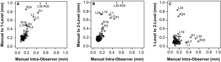
Landmark error comparisons – manual intra‐observer error is the average distance between landmark locations from landmark placement trials 1 and 2 across a representative subset of 100 samples. Average intra‐observer error is compared to the average distances between (A) manual and one‐level landmark coordinates, (B) manual and two‐level landmark coordinates and (C) one‐level and two‐level landmark coordinates for each landmark across all samples. Landmarks showing relatively high placement error are identified by ID, as defined in Fig. 2.

With intra‐observer error as a baseline, a comparison of manual landmark placement and one‐level or two‐level‐based automated landmark placement was completed. The mean differences between automatic and manual landmark placement are between 0.11 and 1.37 mm for one‐level (Fig. 4A), and between 0.11 and 1.54 mm for two‐level procedures (Fig. 4B). L/R1, L/R3 and L/R35 are again among the landmarks with the highest error. In addition, landmarks L/R19, L/R24 and L/R15 show relatively high automated landmarking error. Overall, the mean landmark placement error and standard deviation of that error for a given landmark is higher for automated than for manual landmarking, although 45 of 68 mean automated errors still met our criteria of 0.25 mm for one‐level registration and 50 of 68 for two‐level registration (Table 3, Fig. 4A,B). In addition to differences between automated and manual landmark placement, automated results for most landmarks include several outlier specimens with relatively poor accuracy of automated landmark identification (Supporting Information Fig. S1). Outlier specimen identity varies between landmarks.

Because a portion of the difference in average manual and automated landmark positions is based in manual landmark placement error, we subtracted mean intra‐observer error to produce conservative estimates of the mean automated landmarking error in identifying the correct position of each anatomical landmark. Landmarks L/R1, L/R3, L/R19, L/R24, L/R35 each have > 0.25 mm mean automated placement error for at least one of the automated methods after accounting for manual landmarking error (Table 3). These landmarks are found on the anterior portion of the face or on the zygomatic arch. Each of these 10 landmarks were removed from the dataset before completing subsequent Procrustes superimposition‐based analyses.

The mean distances between landmarks identified with one‐level and two‐level automated methods are shorter than the distances between manual and automated landmarks. These mean differences in landmark placement between our automated methods are quite comparable to intra‐observer error values, except for landmark L/R24, which shows a difference in one‐ and two‐level automated placement that is approximately 0.8 mm (Figs 4C and S1).

Impact of landmarking method on skull shape summary measures

Procrustes superimposition of specimen landmark coordinates from a combination of manual, one‐level and two‐level methods was completed to quantify the influence of landmarking method on morphometric analyses of skull shape. After superimposition, it was noted that the strongest skull shape outlier specimens displayed errors in the automated identification of L/R16 and M36 along the foramen magnum because of the false identification of the first vertebrae as part of the skull during image registration. This serious registration error appears to have occurred for a minority of specimens.

A nested Procrustes anova indicates that approximately 65% of landmark variance represents inter‐specimen variation and 35% represents variation in landmark identification between landmarking methods. The influence of landmarking method is also highlighted with a PCA of this combined dataset for which the second PC (14% of variance) is associated with a separation between manual and automatic measurement methods, and the fourth (7%) is associated with separation of all three measurement methods. The first (18%) and third (8%) PCs are associated with genotype variation shared across methods (Fig. 5). When landmark locations are visualized after Procrustes superimposition, automated landmarks frequently cluster slightly away from manual landmarks (Supporting Information Fig. S2).

Figure 5.

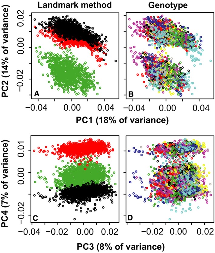
Principal components of all samples and methods – visualization of all specimens along principal components (PCs) (A) 1 & 2 and (C) 3 & 4 from an analysis including landmark coordinates from manual (green), one‐step (black) and two‐step (red) landmarking methods. This illustrates separation of specimens by landmarking method along PCs 2 and 4. (B,D) The same plots, but with each of 64 genotypes randomly identified by one of eight rainbow colors. This is meant to illustrate similarities in genotype distribution along PCs 1 and 3 for each landmarking method.

Estimates of Procrustes shape variance and covariance structure

If differences in shape estimates between methods are consistent across all specimens, then the automated landmarking method results might provide accurate estimates of biological variation and covariation in our sample. Genotype‐specific Procrustes shape variance is approximately two times lower for automated landmarks than for manual landmarks (Fig. 6A), meaning that variation present in manual landmarks is not present in automated landmarks. Kendall's rank correlation tests indicate a significant, albeit not particularly strong, positive correlation between the manual and automatic landmark‐derived Procrustes variances between manual and one‐level (tau: 0.359, P < 0.0001) (Fig. 6B) or two‐level (tau: 0.308, P < 0.0001) methods. Comparisons of variance‐covariance matrices by method revealed that the covariance structure of one‐level and two‐level automated landmarks are broadly similar to the covariance structure of manual landmarks, with matrix correlations of approximately 0.7 (Table 4). The similarity of covariance structure between the two automated methods is very high (matrix correlations: 0.97).

Figure 6.

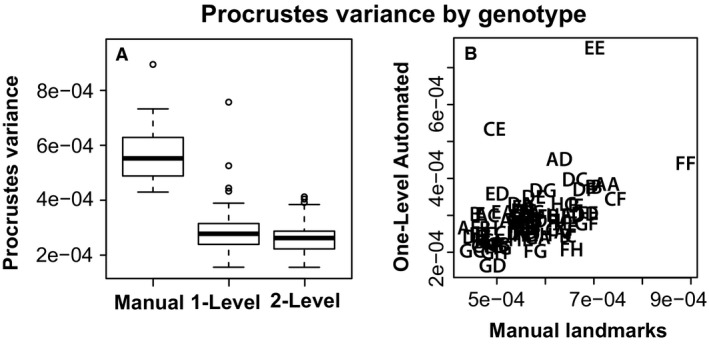
Genotype specific shape comparisons – (A) Genotype specific comparisons of Procrustes variance of skull shapes estimated from manual, one‐level and two‐level landmarking methods. (B) Correlation between genotype‐specific Procrustes variance of skull shapes estimated from manual and one‐level automated landmarking methods.

Table 4.

Comparisons of covariance structure among methods using random skewers and matrix correlations for individual‐level variation as well as the genotype means

	Random skewers		Matrix correlation
	Manual	1‐level	Manual	1‐level
Individual‐level variation
1‐level	0.67*		0.70*
2‐level	0.73*	0.97*	0.73*	0.98*
Genetic covariance
1‐level	0.66*		0.67*
2‐level	0.69*	0.97*	0.71*	0.97*

^*All correlations are significant at P < 0.001.

Separate PCAs were conducted for the manual, one‐level and two‐level Procrustes landmarks to compare the major axes of skull shape covariance identified with different methods (Fig. 7). The eigenvalues of the first few PCs are similar across methods and their scores correlate fairly well for PCs 1‐3 and 5 (Fig. 7D,E). A higher proportion of total variation is explained by the first two automated method PCs than the first two manual landmark PCs. Similarity in early PC eigenvalues across methods suggests that the higher shape variance estimated from manual landmarks is disproportionately distributed in later PCs. Overall, the earliest PCs of manual landmark coordinates and automated landmark coordinates capture correlated axes of shape covariation. Correlations between manual and automated PC scores are substantially increased when method‐specific PCAs are completed on mean genotype shape coordinates rather than all specimen coordinates (Supporting Information Figs S3 and S4).

Figure 7.

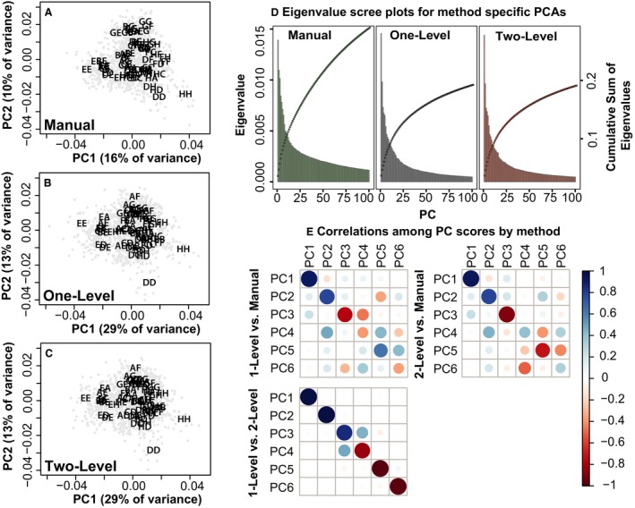
Principal components by method – visualization of specimens (gray circles) and genotype means (abbreviations from Table 2) along principal components (PCs) 1 and 2 of separate principal component analyses of specimen landmark data from (A) manual, (B) one‐level and (C) two‐level landmarking methods. (D) Scree and cumulative eigenvalue plots for these principal components analyses. (E) Correlation plots for the first six PC scores from these analyses.

To determine whether inter‐genotype differences identified from manual landmarks are similarly identified from automated landmarks, we computed the Procrustes distances between mean genotype shapes within each method. The distributions of these distances (Fig. 8A) reveal extensive overlap between methods, but there was a tendency for manual landmark‐based distances among genotypes to be larger (anova, df = 11 346, F = 748, P < 1 × 10⁻¹⁶). Across methods, however, the relative distances correspond very well (Fig. 8B), revealing correlations of 0.93 between manual and automated inter‐genotype distances and of 0.99 between one‐level and two‐level automated methods. Generally, genotypes that are identified as more different based on manual landmarks are also identified as more different based on automated landmarks.

Figure 8.

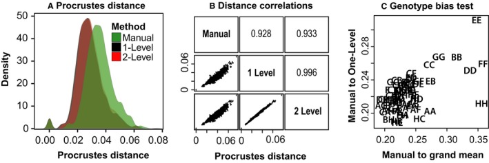
Procrustes distances among genotypes by method. (A) The full distributions of among‐genotype distances by method. (B) Correlations of among‐genotype Procrustes distances pairwise by method. (C) Comparison of the Procrustes distances (overall magnitude of shape differences) between genotype‐specific skull shapes and the overall average skull shape as estimated from manual landmarks (x‐axis) vs. the Procrustes distances between genotype‐specific skull shapes as calculated from manual and one‐level automated landmarking methods (y‐axis).

Genotype‐specific biases on the impact of automatic landmarking

There are broad similarities in inter‐genotype skull shape comparisons based on automated and manual landmarking methods. But, it is important to understand whether differences in shape estimates produced by these methods include any genotype‐specific biases that might lead to different conclusions about inter‐genotype variation. A Procrustes anova with genotype, landmarking method and their interaction as factors indicates that 6% of total landmark coordinate variation is associated with interaction between genotype and landmarking method (Table 5). For comparison, genotype is associated with 41% and landmarking method with 20%. The significant interaction effect suggests a bias in how the automated method identifies landmarks in certain genotypes. To test the hypothesis that genotypes with mean shapes found farther from the grand mean shape show higher levels of automated landmark placement error, we looked for a correlation of (1) the distance between manual genotype mean shape and the manual grand mean shape and (2) the distance between manual genotype mean shape and one‐level automated genotype mean shape. There was a significant positive correlation whether we compared manual landmark data with one‐level (0.584, P < 0.001) or two‐level (0.550, P < 0.001) landmark data. These correlations may be driven largely by the particularly high genotypic divergence of some of the founder strains from the manual grand mean shape (Fig. 8C).

Table 5.

Results from a Procrustes anova with genotype, landmarking method (i.e. manual, one‐level, two‐level), and the interaction of genotype and landmarking method as factors

	df	SS	MS	R2	F	Z	Pr (>F)
Genotype	61	1.615	0.026	0.405	67.320	29.619	0.001
Landmark method	2	0.784	0.392	0.197	996.430	21.407	0.001
Geno × method	122	0.237	0.002	0.059	4.930	30.105	0.001
Residuals	3429	1.348	0.000
Total	3614	3.983

df, degrees of freedom; MS, mean squares; SS, sum‐of‐squares, with R² interpreted as proportion of variation associated with a factor.

The source of increased skull shape variance in manual landmark estimates

The observation that the additional manual landmark variance is associated with lower‐order PCs is consistent with the hypothesis that this variation represents measurement error. However, the lower variance in automated method lower‐order PCs could instead be due to an inability of automated landmarking to capture subtle features of biological variation. To test this, we broke manual landmark data multivariate variation into a component that is also represented in one‐level automated landmark data and a component that is not. A manova for genotype was completed on the component of manual variation not shared with the automated method to determine how much of this residual manual variation can be explained by genotype identity. This analysis indicated that regressing out the automated landmark covariance structure removed 70% of the total variance in the manual data (covariance matrix trace, i.e. sum of variances, changed from 0.0012 to 0.00036) (Table 6). In other words, about 70% of the manual landmark variance corresponds to what is captured by automated landmarking. The remaining variation does show significant variation by genotype, but manova by genotype revealed that the variation attributable to genotype is reduced by 96% and the variance explained by genotype drops from over 50% to 7% of the total variance. If the manual landmark residuals are removed from the original manual landmark data, genotype still accounts for 69% of the total variance. This strongly suggests that although some of the loss of variation in automated compared with manual landmarks may correspond to biological signal, the majority of this loss is due to the minimization of measurement error within the automated method.

Table 6.

Variances attributable to genotype as estimated by manova for automated landmarking, manual landmarking, and manual landmarking after removing the variation captured by automated landmarking

Dataset	Total variance	Genotype variance	Genotype variance (%)
One‐level automated	0.00073	0.0043	60
Two‐level automated	0.00071	0.0044	63
Full manual data	0.00122	0.0065	54
Manual data residual variance after automated lm variance‐covariance removed	0.00036	0.0003	7
Manual data residual variance after automated lm regression residuals removed	0.00086	0.0059	69

Statistical power comparison

A simulation to compare the statistical power of landmarking methods to detect skull shape differences between genotypes revealed only minimal differences in statistical power (Fig. 9). In each iteration of our simulation, groups were compared by manova as were both the method‐specific differences in the estimates of the among‐group and the within‐group variances, and covariances are considered. To account for the fact that automated landmarking reports lower Procrustes distances among groups, we used the among‐group Procrustes distances as determined by manual landmarking as the independent variable. The two variants of the automated landmarking method did not differ in statistical power, but both performed slightly better than manual landmarking. These results suggest that there is no loss of power with automated landmarking.

Figure 9.

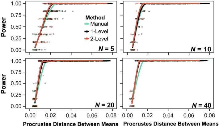
Statistical power simulations – Statistical power simulations for n = 5, 10, 20 and 40 specimens per genotype. Each plot shows power relative to Procrustes distance between genotypes. For comparison, the mean Procrustes distance among genotypes as determined by manual landmarking is 0.035. In the simulation, 100 samples were generated at each sample size with the method‐specific variance‐covariance structures for each genotype. Within each method and sample size‐specific sample, all possible pairwise comparisons among genotypes were performed using manova to generate the power curves.

We tested our assumption that the repeatability of variance‐covariance matrices are similar across methods by resampling all genotype groups with replacement. The repeatability values do vary by method (anova, df = 18 414, F = 4022, P < 1 × 10⁻¹⁶), with manual landmarking having the lowest repeatability (by 30%). Since the repeatability of the variance covariance matrix was not built into our power simulation, this means that the power estimates for the manual data are likely overestimated and so the automated landmark data likely perform better than manual landmarking in terms of distinguishing groups. This is consistent with the fact that biological variation represents a larger proportion of the total variance in automated landmark data (Table 6).

Discussion

Well‐chosen anatomical landmarks represent the shape and size of an object, serving as the basis for in‐depth morphometric comparisons. Although anatomical landmarks may not encompass all aspects of object shape, the homology of those landmarks across samples allow morphometric results to be directly tied to specific biological and geometric features of interest. The possibility of accurate automatic anatomical landmark identification is enticing because manual identification is time‐consuming and tedious. In addition, the presence of inter‐observer error means that comparisons of manual landmarks collected across multiple studies can be problematic, even if the same landmark definitions were used for each study. Automation of landmark identification may save time and allow for direct comparisons of landmarks collected across many years and between different research groups. To assess the accuracy of automated landmark identification and subsequent analytical results for a large sample with high levels of variation, we tested two procedures that combine affine and non‐linear registration of mouse skull μCT images to iteratively defined average images. Our results reveal significant differences in manually and automatically identified landmarks, although similar broad patterns of skull shape covariation are identified from landmarks produced using each method. Additionally, automated landmarks do not include the intra‐observer error noted for manual landmarks and display similar statistical power in differentiating genotypes by skull shape.

Landmark error

Mean intra‐observer errors for most landmarks are below 0.25 mm (Table 3), which is equivalent to 7 voxel lengths in our original images and shorter than the medial‐lateral width of the jugal bone of the zygomatic arch in C57BL/6J mice (~ 0.35 mm). This degree of landmark error, as measured in number of voxels, is similar to the intra‐observer error previously accepted during placement of embryonic facial surface landmarks (Percival et al. 2014). However, the high intra‐observer error noted for a few landmarks (L/R1, L/R3 and L/R35) likely represents a systematic shift in our expert's landmark identification over the 4 years between manual landmark trial one and trial two.

The mean distance between manual landmark position and automated landmark position is typically larger than the intra‐observer error for a landmark. This suggests that automated methods do not identify anatomical landmarks in the same way as manual methods. This distance measure represents a combination of local image registration error during the automated process and variation in manual landmark placement. The reference landmarks that form the basis for automated landmark positions were recently placed by our expert observer, so they are probably more like manual landmark positions from trial two than from trial one. Therefore, the large distances between manually (based on manual trial one) and automatically identified L/R1, L/R3 and L/R35 positions are likely inflated by the intra‐observer shift in manual landmark identification.

Subtracting mean intra‐observer error from the distance between manual and automated landmark positions provides a conservative estimate of the error of the automated method in accurately identifying anatomical landmarks. After subtracting intra‐observer error for most automatically identified landmarks, the performance of our automated landmark estimation procedure from single atlases showed similar or slightly higher landmark placement error than did previously reported multi‐atlas procedures built for samples from a small number of genotypes (Bromiley et al. 2014; Young & Maga, 2015). However, L/R1, L/R3 and L/R35 still display high automated error (> 0.25 mm), as do L/R19 and L/R24.

Each of these high error landmarks are found on the face or zygomatic arch. The suture margins upon which L/R19 and L/R24 are defined are not visible within the one‐ or two‐level atlases. This suggests a high level of morphological variation in these areas and/or a poor local alignment during the registration process. In fact, the position of L/R24 between two zygomatic arch bones is known to be variable across ‘normal’ mouse skulls (Percival et al. 2018) and the geometrically complex premaxilla‐maxillary suture that defines L/R19 is frequently difficult to visualize in individual specimen μCT images. This lack of a discernible suture in the atlas image is more problematic for L/R24 because there are very few other aspects of zygomatic morphology to guide local alignment. Additionally, the lack of a suture in the atlas images makes it difficult to identify reference landmark position, which might exacerbate the effects of poor alignment on automatic landmark placement.

Previous analyses of MRI registration‐based volume segmentation indicate that higher registration errors are found at the outer edges of the brain rather than in deeper regions (Kovačević et al. 2004). Similarly, L/R35, L/R1 and L/R3 are found near the anterior ends of the face and zygomatic process of the maxilla, where there are no surrounding regions of the skull to constrain local deformation. It is likely that poor local image alignments at variable suture margins and the anterior end of facial bones help explain the high automated landmark placement error for these landmarks. This supports our expectation that landmarks with high automatic landmark placement error would be found in regions with more image alignment error. Unfortunately, the landmarks that represent the most interesting regions of morphological variation might also be the most problematic to identify automatically, due to high levels of inter‐specimen variation. Landmarks in these regions should probably be removed from analysis, as we did for the high automated error landmarks before performing Procrustes superimposition.

After subtracting intra‐observer error, most mean automated landmark error estimates are below the 0.25 mm intra‐observer cutoff. However, high standard deviations in the distance between manual and automated landmark locations indicate lower consistency in automatic landmark placement for some landmarks (Table 3). High standard deviations partially reflect a relatively high number of landmark placement outliers noted for the automated process (Fig. S1). Aside from a handful of catastrophic image registration errors that were identified and removed prior to analysis, the outliers in automated landmark placement appear to represent stochastic instances of local registration error. For example, the biggest specimen outliers have major errors in landmark placement around the foramen magnum (L/R16, M36) because the first cervical vertebra was accidentally identified as part of the skull during the registration procedure. There do not appear to be other correlated landmark position errors apart from the foramen magnum in these particular outlier specimens. Careful consideration of the outlier specimens in a shape analysis would help to identify other serious instances of local registration error. Unfortunately, relying on lists of potential outliers (based on large differences from mean shape) may not be enough to identify less serious instances of registration error within samples that include a high amount of real biological variation, as exists among our 62 genotypes. The best strategy to solve these types of stochastic registration errors is to completely and precisely standardize specimen preparation, mounting during image acquisition, and image processing that occurs prior to the registration pipeline.

Impact of landmarking method on analysis

Automated landmark positions do not always match manual landmark positions. Even after removing the high automated error landmarks, a nested Procrustes anova indicates that landmarking method explains 35% of landmark coordinate variation in our combined sample. A PCA of the same dataset also reveals clear separation between methods in landmark identification (Fig. 5). It is obvious that the one‐level and two‐level registration‐based automated landmarking methods identify anatomical landmarks differently than our expert observer, even though our expert observer also provided the reference landmarks for the automated process. However, if there is a general consistency in how the automated method differs from the manual, perhaps in the same way that two expert observers can differ in manual placement, the results of morphometric analyses of automated and manual landmarks should be comparable.

Similar clustering of specimens by genotype (color) are noted along PCs 1 and 3 of the combined PCA of all specimen landmarks (Fig. 5B,D). Comparisons of PCAs completed for each landmarking method separately show correlations in specimen PC scores for several early PCs. This indicates a similarity of measured skull shape covariation for automatically and manually collected landmarks (Fig. 7). When PCAs are completed on genotype mean shapes rather than specimens individually, PC score correlations are much higher (Fig. S1). This increased correlation may be due to the fact that mean manual landmark genotype shapes are largely free of stochastic intra‐observer error.

Although specific landmark positions may differ between methods, the general patterns of skull shape variation identified are similar between methods. Registration‐based automatic landmark analysis of skull shape variation by Maga et al. (2017) showed a similar result. Therefore, these types of automated landmarking methods can be used to identify accurately general inter‐genotype differences in skull shape noted across common laboratory mouse strains. However, there are genotype specific biases in the difference between skull shape estimates produced with manual and automated landmarks. Genotypes with skull shapes least similar to grand mean average skull shape are those for which automatic landmark estimates of skull shape are most different from manual landmark‐estimated skull shape (Fig. 8C). This suggests that genotypes with more divergent phenotypes display less accurate skull shape estimates, likely due to underestimation of the actual degree of divergence from the atlas image. This matches previous results showing that the largest simulated changes in organ volume were underestimated by similar image registration procedures (van Eede et al. 2013). The use of multi‐atlas registration methods may help to reduce the severity of this issue.

One‐level vs. two‐level

Given the relatively wide range of skull variation noted in our sample, we expected that the two‐level registration method would produce more accurate local image registration and landmark placement than the one‐level method. Inbred mouse strain specific averages have been previously applied during an analysis of C57BL/6J and 129S1/SvImJ mouse embryos (Zamyadi et al. 2010). We found a systematic difference between the results of the two procedures, as revealed by separation along PC 4 of the PCA of all specimens and methods (Fig. 5C). However, the distances between one‐level‐ and two‐level‐identified landmark positions are comparable to the acceptable range of intra‐observer error (Table 3; Fig. 4). In addition, the correlations of PC scores (Fig. 7E) and Procrustes distances between genotypes (Fig. 8A,B) between automated methods are high. The results of both automated methods are quite similar.

The significant correlation between more extreme morphology (typically of founder strains) and the level of automated landmark placement error (Fig. 8C) may be evidence of poorer image registration for specimens with more extreme phenotypes. We expected strain‐specific bias in image registration might be reduced using a two‐level registration procedure. However, the correlation between extreme shape and automated error was similar for both one‐level and two‐level results. At least for the range of skull shape variation in our current sample, the one‐level procedure appears to perform as well as the two‐level procedure. The application of one‐level or multi‐level registration methods to samples with greater intra‐genotype variation, including mouse mutants or different mouse species, should be separately validated.

When possible, a one‐level procedure should be preferred over a two‐level procedure because all specimens of all genotypes will be aligned to the same image averages at all steps. In the two‐level procedure, all specimens of a given genotype are registered to a genotype‐specific average during the first level and that average is registered to the overall average in the second‐level. Therefore, any artifactual differences in registration during the second‐level procedure will modify the results for all specimens of a given genotype in the same way. These types of registration artifacts will be confounded with real biological differences between genotypes in any subsequent analysis.

Procrustes shape variance

Although there are correlated patterns of Procrustes shape between manual and automated datasets (Table 4, Fig. 7), genotype‐specific Procrustes shape variance is approximately two times lower for all genotypes (Fig. 6A). Part of this reduction is likely due to the higher precision (not necessarily accuracy) inherent in automated methods. Given identical inputs, an algorithmic landmarking method is expected to place a landmark in the same place each time it is run, whereas expert observers always display some intra‐observer placement error. The reduced shape variance may also reflect an underestimation of real biological variation. Previous simulations of major brain region volume expansion and reduction, for example, showed consistent underestimation of simulated changes by approximately 60% when using similar image registration methods (Pieperhoff et al. 2008; van Eede et al. 2013). Therefore, we expected that estimated differences between genotype‐specific skull shape and overall average skull shape would be underestimated by our automated landmarks. This is borne out in our analysis, which shows that the shape distances among genotypes are, on average, 25% lower with automated landmarking (Fig. 8A). Since intra‐observer measurement error is unlikely to artificially inflate among‐genotype differences in the manual data, the contraction of variance in automated data is not likely to be due to the greater precision of automated landmarking.

Despite the contraction of variance, our analyses show that statistical power to differentiate genotypes by skull shape is conserved, if not slightly increased, with automated landmarking (Fig. 9). This suggests that at least some of the loss of variance is due to reduced measurement error. Supporting this idea is the fact that additional variance in manual landmarking is distributed across the smaller principal components (Fig. 7D), whereas the major aspects of covariation structure are very similar (Fig. 7E). Furthermore, the component of manual landmark data that does not overlap with automated landmark data (i.e. the portion of manual landmark variance‐covariance not found in the automated data) is not explained well by specimen genotype identity (Table 6). Finally, the component of the manual data that corresponds to the automated landmark variance‐covariance structure contains proportionately more variation related to genotype than the automated datasets. These results suggest strongly that a large proportion, but not all, of the difference in variance magnitude between manual and automated landmarking is due to manual intra‐observer measurement error. Our automated landmarking method produces a favorable tradeoff, in that the loss of biological variation is outweighed by the reduction in random error.

Accurate estimates of morphological variance and differences in levels of variance are as critical as differences in mean morphology when answering some research questions. For example, cross‐breeding studies indicate that hybrid mice display lower variation within as well as between genotypes compared with their inbred parental strains (Leamy, 1982). Also, mouse models of craniofacial diseases with known mutations have frequently shown higher degrees of within group variation than related control mice do (reviewed in Hallgrímsson et al. 2009). Careful quantification of changes in related genes have recently provided important evidence for non‐linear developmental systems of complex traits, including craniofacial morphology (Hallgrimsson et al. 2018). The reduction in apparent variance with automated landmarking implies that it would be highly problematic to mix manual and automated landmark data in analyses focused on comparisons of phenotypic variance.

Automatic or manual landmarks

Sophisticated image registration and analysis paradigms, such as deformation‐, tensor‐ and voxel‐based morphometry, have been developed to quantify and compare brain morphology from MRIs in a precise and replicable fashion. Common applications within the study of morphometry, including automated segmentation of particular regions (Ashburner & Friston, 2000), analysis of deformation fields and the production of parametric maps via voxel‐by‐voxel comparisons (Friston et al. 1994; Penny et al. 2011), typically leverage the coordinate transformations embedded within a registration workflow to detect global and local changes in brain size, shape and form. As part of a larger interdisciplinary program on anatomical variation, these methods have also been successfully applied to compare the volumes of other organs within contrast‐enhanced computed tomography images (Wong et al. 2012). The results of our study and others (Bromiley et al. 2014; Young & Maga, 2015; Maga et al. 2017) indicate that using automated image registration techniques as a basis for anatomical landmark collection can produce broadly similar morphometric results to landmarks collected manually by expert observers. An automated image registration pipeline can provide many benefits. First, it can provide consistency in phenotypic quantification over many years, removing the possibility of intra‐observer landmark placement drift. As highlighted by Maga et al. (2017), the use of the same image registration pipelines and image atlases by multiple labs can allow for direct comparisons of morphometric results between studies and labs. The sharing and critical evaluation of annotated image atlases (aka templates) will be required to make this a reality, because the choice of atlas will have a significant effect on morphometric results (Aljabar et al. 2009). Secondly, for large studies, automated phenotyping can remove the time‐consuming need for single, trained observers to collect all measurements. Thirdly, once image registrations have been completed for a sample, the resulting transformations can be used to identify anatomical landmarks and to complete a variety of other quantifications including volume estimation and deformation‐based comparisons.

The use of image registration and automated landmarking is very appealing but its successful implementation includes assumptions and pitfalls that do not exist for the collection or analysis of manually identified landmarks. Most importantly, an automatically identified anatomical landmark may not retain the precise homology it had when it was collected manually (Fig. S2). Although an anatomical landmark may represent a biological feature of interest to an expert observer, the voxel upon which a landmark is identified is simply one among thousands within a registered image. Common image registration methods do not have any expert anatomical knowledge built into them (Avants et al. 2008). They are based on matching gradients and contrast borders within each image. Consequently, a registration‐based procedure may place a landmark in a position that no expert observer would ever place it, even if it is very close to the manually identified position. For example, a landmark might be identified a couple of voxels deep to the bone surface; it may only be 0.1 mm away from the actual position, but the placement inside a bone rather than on the bone surface might be disconcerting for an anatomist. Although algorithmic rules can be employed to make sure that each landmark is moved to the nearest bone surface, this may move the landmark farther away from the accurate position, particularly when landmarks are on thin skull bones. Consistent differences between the automated and manual landmark placement noted in our results are analogous to inter‐observer differences caused by varied interpretations of where to place a given landmark.

Major stochastic differences in landmark position noted after Procrustes superimposition, as exist for foramen magnum landmarks in some of our specimens, indicate error in landmark placement that is due to unexpected differences across the input images. In this case, a combination of the distance and the angle between the occipital bone and the first few vertebrae in some images led to the identification of the caudal end of the first vertebrae as the edge of the foramen magnum. Image registration methods assume that all specimens have exactly the same structures in the same relative positions (Wong et al. 2012). Exceptions to this assumption can come in the form of imaging artifacts or natural biological variation (e.g. major disease phenotypes or evolutionary differences).

For natural biological variation, the use of alternative algorithms, such as multi‐atlas procedures (Aljabar et al. 2009; Chakravarty et al. 2013; Wang et al. 2013; Bromiley et al. 2014; Young & Maga, 2015) or neural‐network methods (Zheng et al. 2015), may prove more robust to variation across our sample. Neural network methods may be particularly amenable to identifying anatomical landmark position, because the number of variables to estimate is low relative to 3D volume segmentation procedures. The use of a preliminary pairwise‐nonlinear registration step might also improve image registration for regions of the skull with high variability by improving early image alignments. Given that our image registration pipeline was previously optimized for organ volume segmentation, it is possible that modifications to algorithm parameters during image registration may improve automated landmark placement accuracy without the need for major changes to the reported pipeline.

For variation caused by imaging artifacts, error can be reduced by making sure that the morphology found within all input images is directly comparable. This may be easiest to do by standardizing the position of each specimen during image acquisition, including the orientation of the mandible and vertebrae relative to the skull. Alternatively, if a researcher is only interested in the cranium, they might consider the careful removal of the whole vertebral column and the mandible before image acquisition, perhaps using a dermestid beetle colony.

Although the use of an automated landmarking method can remove the time investment required for manual landmarking, it requires an increase in the effort and care required during specimen processing, image acquisition and quality control to identify successfully instances of imaging and image registration error. Given the fact that automated and manual landmarks are placed significantly differently, it is critical not to combine manual and automated landmarks in a single analysis. When automated placement error is identified, it might be tempting to move the landmark position manually. However, this should be considered analogous to introducing inter‐observer error into a landmark dataset.

Conflict of interest

The authors have no conflicts of interest to declare.

Author contributions

C.J.P. – study design, data collection, data analysis, manuscript drafting, editing and approval of manuscript. J.D. – data collection, manuscript contributions, editing and approval of manuscript. B.D. – manuscript contributions, editing, and approval of manuscript. W.L. – data collection, manuscript editing, and approval of manuscript. M.v.E. – study design, data collection, manuscript editing, and approval of manuscript. R.M.H. – study design, manuscript editing, and approval of manuscript. B.H. – study design, data analysis, manuscript editing, and approval of manuscript.

Supporting information

Fig. S1. (a) Left side landmarks. (b) Right side landmarks. (c) Midline landmarks.

Fig. S2. Manual and one‐step automated procrustes landmark position.

Fig. S3. Principal components of genotype mean shapes, comparing methods.

Fig. S4. Comparisons of PCs from PCAs of genotype mean skull shape completed separately for each landmarking method (as in Fig. S3)

Appendix S1. A .csv file with landmark coordinates as identified, by one‐level, and by two‐level automated methods are available in a file called “SupFileCoords.csv”.

References

- Adams DC, Collyer ML, Kaliontzopoulou A, et al. (2016). geomorph: Software for geometric morphometric analyses. R package version 3.0.2 [WWW Document]. URL http://cran.r-project.org/web/packages/geomorph/index.html
- Aldridge K, Boyadjiev SA, Capone GT, et al. (2005) Precision and error of three‐dimensional phenotypic measures acquired from 3dMD photogrammetric images. Am J Med Genet A 138, 247–253. [DOI] [PMC free article] [PubMed] [Google Scholar]
- Aljabar P, Heckemann RA, Hammers A, et al. (2009) Multi‐atlas based segmentation of brain images: atlas selection and its effect on accuracy. NeuroImage 46, 726–738. [DOI] [PubMed] [Google Scholar]
- Ashburner J, Friston KJ (2000) Voxel‐based morphometry – the methods. NeuroImage 11, 805–821. [DOI] [PubMed] [Google Scholar]
- Avants BB, Epstein CL, Grossman M, et al. (2008) Symmetric diffeomorphic image registration with cross‐correlation: evaluating automated labeling of elderly and neurodegenerative brain. Med Image Anal 12, 26–41. [DOI] [PMC free article] [PubMed] [Google Scholar]
- Avants BB, Tustison NJ, Song JCG (2009). ANTS: advanced open‐source normalization tools for neuroanatomy. Philadelphia: Penn Image Computing and Science Laboratory.
- Avants BB, Tustison NJ, Song G, et al. (2011) A reproducible evaluation of ANTs similarity metric performance in brain image registration. NeuroImage 54, 2033–2044. [DOI] [PMC free article] [PubMed] [Google Scholar]
- Beck JA, Lloyd S, Hafezparast M, et al. (2000) Genealogies of mouse inbred strains. Nat Genet 24, 23–25. [DOI] [PubMed] [Google Scholar]
- Benedikt H, Boughner JC, Turinsky A, et al. (2009) Geometric morphometrics and the study of development In: Advanced Imaging in Biology and Medicine (eds. Sensen CW, Hallgrímsson B.), pp. 319–336. Berlin: Springer. [Google Scholar]
- Bookstein FL (1991) Morphometric Tools for Landmark Data: Geometry and Biology. Cambridge, UK: Cambridge University Press. [Google Scholar]
- Boyer DM, Puente J, Gladman JT, et al. (2015) A new fully automated approach for aligning and comparing shapes. Anat Rec 298, 249–276. [DOI] [PubMed] [Google Scholar]
- Bromiley PA, Schunke AC, Ragheb H, et al. (2014) Semi‐automatic landmark point annotation for geometric morphometrics. Front Zool 11, 1.24401080 [Google Scholar]
- Chakravarty MM, Aleong R, Leonard G, et al. (2011) Automated analysis of craniofacial morphology using magnetic resonance images. PLoS ONE 6, 1–13. [DOI] [PMC free article] [PubMed] [Google Scholar]
- Chakravarty MM, Steadman P, van Eede MC, et al. (2013) Performing label‐fusion‐based segmentation using multiple automatically generated templates. Hum Brain Mapp 34, 2635–2654. [DOI] [PMC free article] [PubMed] [Google Scholar]
- Chesler EJ, Miller DR, Branstetter LR, et al. (2008) The Collaborative Cross at Oak Ridge National Laboratory: developing a powerful resource for systems genetics. Mamm Genome 19, 382–389. [DOI] [PMC free article] [PubMed] [Google Scholar]
- Churchill GA, Airey DC, Allayee H, et al. (2004) The Collaborative Cross, a community resource for the genetic analysis of complex traits. Nat Genet 36, 1133–1137. [DOI] [PubMed] [Google Scholar]
- Claes P, Walters M, Vandermeulen D, et al. (2011) Spatially‐dense 3D facial asymmetry assessment in both typical and disordered growth. J Anat 219, 444–455. [DOI] [PMC free article] [PubMed] [Google Scholar]
- Claes P, Roosenboom J, White JD, et al. (2018) Genome‐wide mapping of global‐to‐local genetic effects on human facial shape. Nat Genet 50, 414. [DOI] [PMC free article] [PubMed] [Google Scholar]
- Collaborative Cross Consortium (2012) The genome architecture of the Collaborative Cross mouse genetic reference population. Genetics 190, 389–401. [DOI] [PMC free article] [PubMed] [Google Scholar]
- Deans AR, Mikó I, Wipfler B, et al. (2012) Evolutionary phenomics and the emerging enlightenment of arthropod systematics. Invertebr Syst 26, 323–330. [Google Scholar]
- van Eede MC, Scholz J, Chakravarty MM, et al. (2013) Mapping registration sensitivity in MR mouse brain images. NeuroImage 82, 226–236. [DOI] [PubMed] [Google Scholar]
- Friedel M, van Eede MC, Pipitone J, et al. (2014) Pydpiper: a flexible toolkit for constructing novel registration pipelines. Front Neuroinform 8, 1–21. [DOI] [PMC free article] [PubMed] [Google Scholar]
- Friston KJ, Holmes AP, Worsley KJ, et al. (1994) Statistical parametric maps in functional imaging: a general linear approach. Hum Brain Mapp 2, 189–210. [Google Scholar]
- Gower JC (1975) Generalized procrustes analysis. Psychometrika 40, 33–51. [Google Scholar]
- Guo JG, Mei X, Tang K (2013) Automatic landmark annotation and dense correspondence registration for 3D human facial images. BMC Bioinformatics 14, 1–12. [DOI] [PMC free article] [PubMed] [Google Scholar]
- Hallgrímsson B, Jones N (2009) Anatomical imaging and post‐genomic biology In: Advanced Imaging in Biology and Medicine (eds Hallgrímsson B, Sensen CW.), pp. 411–426. Berlin: Springer. [Google Scholar]
- Hallgrímsson B, Jamniczky H, Young NM, et al. (2009) Deciphering the palimpsest: studying the relationship between morphological integration and phenotypic covariation. Evol Biol 36, 355–376. [DOI] [PMC free article] [PubMed] [Google Scholar]
- Hallgrimsson B, Percival CJ, Green R, et al. (2015) Morphometrics, 3D imaging, and craniofacial development In: Craniofacial Development, Current Topics in Developmental Biology (ed. Chai Y.), pp. 561–597. Waltham: Elsevier Academic Press. [DOI] [PMC free article] [PubMed] [Google Scholar]
- Hallgrimsson B, Green RM, Katz DC, et al. (2018) The developmental‐genetics of canalization. Semin Cell Dev Biol 1–13. Elsevier. 10.1016/j.semcdb.2018.05.019. [DOI] [PMC free article] [PubMed] [Google Scholar]
- Houle D, Govindaraju DR, Omholt S (2010) Phenomics: the next challenge. Nat Rev Genet 11, 855–866. [DOI] [PubMed] [Google Scholar]
- Jamniczky HA, Hallgrímsson B (2009) A comparison of covariance structure in wild and laboratory muroid crania. Evolution 63, 1540–1556. [DOI] [PubMed] [Google Scholar]
- Kohn L, Cheverud J (1992) Calibration, validation, and evaluation of scanning systems: anthropometric imaging system repeatability In: Electronic Imaging of the Human Body Workshop pp. 114–123. Dayton: Crew System Ergonomics Information Center. [Google Scholar]
- Kovačević N, Henderson J, Chan E, et al. (2004) A three‐dimensional MRI atlas of the mouse brain with estimates of the average and variability. Cereb Cortex 15, 639–645. [DOI] [PubMed] [Google Scholar]
- Leamy L (1982) Morphometric studies in inbred and hybrid house mice II. Patterns in the variances. J Hered 73, 267–272. [DOI] [PubMed] [Google Scholar]
- Lele S, Richtsmeier JT (2001) Chapter 2: morphometric Data In: An Invariant Approach to Statistical Analysis of Shapes pp. 15–60. Boca Raton: Chapman & Hall. [Google Scholar]
- Lerch JP, Sled JG, Henkelman RM (2011) MRI phenotyping of genetically altered mice. Methods Mol Biol 711, 349–361. [DOI] [PubMed] [Google Scholar]
- Li M, Cole JB, Manyama M, et al. (2017) Rapid automated landmarking for morphometric analysis of three‐dimensional facial scans. J Anat 230, 607–618. [DOI] [PMC free article] [PubMed] [Google Scholar]
- Loken C, Gruner D, Groer L, et al. (2010) SciNet: lessons learned from building a power‐efficient top‐20 system and data centre. J Phys: Conf Ser 256, 012026. IOP Publishing. [Google Scholar]
- Maga AM, Tustison NJ, Avants BB (2017) A population level atlas of Mus musculus craniofacial skeleton and automated image‐based shape analysis. J Anat 231, 433–443. [DOI] [PMC free article] [PubMed] [Google Scholar]
- Mantel N (1967) The detection of disease clustering and a generalized regression approach. Can Res 27, 209–220. [PubMed] [Google Scholar]
- Marroig G, Cheverud JM (2001) A comparison of phenotypic variation and covariation patterns and the role of phylogeny, ecology, and ontogeny during cranial evolution of New World monkeys. Evolution 55, 2576–2600. [DOI] [PubMed] [Google Scholar]
- Mazziotta JC, Toga AW, Evans A, et al. (1995) A probabilistic atlas of the human brain: theory and rationale for its development: the International Consortium for Brain Mapping (ICBM). NeuroImage 2, 89–101. [DOI] [PubMed] [Google Scholar]
- Nieman BJ, van Eede MC, Spring S, et al. (2018) MRI to assess neurological function. Curr Protoc Mouse Biol 8, e44. [DOI] [PubMed] [Google Scholar]
- Norris FC, Wong MD, Greene ND, et al. (2013) A coming of age: advanced imaging technologies for characterising the developing mouse. Trends Genet 29, 700–711. [DOI] [PubMed] [Google Scholar]
- Ólafsdóttir H, Darvann TA, Hermann NV, et al. (2007) Computational mouse atlases and their application to automatic assessment of craniofacial dysmorphology caused by the crouzon mutation Fgfr2C342Y. J Anat 211, 37–52. [DOI] [PMC free article] [PubMed] [Google Scholar]
- Pavličev M, Mitteroecker P, Gonzalez PN, et al. (2017) Development shapes a consistent inbreeding effect in mouse Crania of different line crosses. J Exp Zool B Mol Dev Evol 326, 474–488. [DOI] [PMC free article] [PubMed] [Google Scholar]
- Penny WD, Friston KJ, Ashburner JT, et al. (2011) Statistical Parametric Mapping: The Analysis of Functional Brain Images. London: Elsevier. [Google Scholar]
- Percival CJ, Green R, Marcucio R, et al. (2014) Surface landmark quantification of embryonic mouse craniofacial morphogenesis. BMC Dev Biol 14, 31. [DOI] [PMC free article] [PubMed] [Google Scholar]
- Percival CJ, Liberton DK, Pardo‐Manuel de Villena F, et al. (2016) Genetics of murine craniofacial morphology: diallel analysis of the eight founders of the Collaborative Cross. J Anat 228, 96–112. 10.1111/joa.12382. [DOI] [PMC free article] [PubMed] [Google Scholar]
- Percival CJ, Green R, Roseman CC, et al. (2018) Developmental constraint through negative pleiotropy in the zygomatic arch. Evodevo 9, 1–16. [DOI] [PMC free article] [PubMed] [Google Scholar]
- Pieperhoff P, Südmeyer M, Hömke L, et al. (2008) Detection of structural changes of the human brain in longitudinally acquired MR images by deformation field morphometry: methodological analysis, validation and application. NeuroImage 43, 269–287. [DOI] [PubMed] [Google Scholar]
- Pomidor BJ, Makedonska J, Slice DE (2016) A landmark‐free method for three‐dimensional shape analysis. PLoS ONE 11, e0150368. [DOI] [PMC free article] [PubMed] [Google Scholar]
- R Developmental Core Team (2008) R: A Language and Environment for Statistical Computing. Vienna: R Foundation for Statistical Computing. [Google Scholar]
- Rohlf FJ (2017) The method of random skewers. Evol Biol 44, 542–550. [Google Scholar]
- Schlager S (2017) Morpho and Rvcg–Shape Analysis in R: R‐Packages for Geometric Morphometrics, Shape Analysis and Surface Manipulations In: Statistical Shape and Deformation Analysis (eds. Guoyan Z, Shuo L, Gabor S.), pp. 217–256. London: Elsevier. [Google Scholar]
- Subburaj K, Ravi B, Agarwal M (2009) Automated identification of anatomical landmarks on 3D bone models reconstructed from CT scan images. Comput Med Imaging Graph 33, 359–368. [DOI] [PubMed] [Google Scholar]
- Talairach J, Tournoux P (1988) Co‐planar Stereotaxic Atlas of the Human Brain: 3‐Dimensional Proportional System: An Approach to Cerebral Imaging. Stuttgart: Thieme Medical Publishers. [Google Scholar]
- Venables V, Ripley B (2002) Modern Applied Statistics with S (eds. Chambers SJ, Eddy W, Hardle W, Sheater S, Tierney L.), New York: Springer Science+ Business Media. [Google Scholar]
- Wang H, Suh JW, Das SR, et al. (2013) Multi‐atlas segmentation with joint label fusion. IEEE Trans Pattern Anal Mach Intell 35, 611–623. [DOI] [PMC free article] [PubMed] [Google Scholar]
- Wilamowska K, Wu J, Heike C, et al. (2012) Shape‐based classification of 3D facial data to support 22q11. 2DS craniofacial research. J Digit Imaging 25, 400–408. [DOI] [PMC free article] [PubMed] [Google Scholar]
- Wong MD, Dorr AE, Walls JR, et al. (2012) A novel 3D mouse embryo atlas based on micro‐CT. Development 139, 3248–3256. [DOI] [PMC free article] [PubMed] [Google Scholar]
- Wong MD, van Eede MC, Spring S, et al. (2015) 4D atlas of the mouse embryo for precise morphological staging. Development 142, 3583–3591. [DOI] [PMC free article] [PubMed] [Google Scholar]
- Young R, Maga AM (2015) Performance of single and multi‐atlas based automated landmarking methods compared to expert annotations in volumetric microCT datasets of mouse mandibles. Front Zool 12, 1–12. [DOI] [PMC free article] [PubMed] [Google Scholar]
- Zamyadi M, Baghdadi L, Lerch JP, et al. (2010) Mouse embryonic phenotyping by morphometric analysis of MR images. Physiol Genomics 42A, 89–95. [DOI] [PMC free article] [PubMed] [Google Scholar]
- Zelditch M, Swiderski D, Sheets DH (2012) Chapter 2: Landmarks and Semilandmarks Geometric Morphometrics for Biologists: A Primer, pp. 23–50. San Diego: Elsevier Academic Press. [Google Scholar]
- Zheng Y, Liu D, Georgescu B, et al. (2015) 3D deep learning for efficient and robust landmark detection in volumetric data In: International Conference on Medical Image Computing and Computer‐Assisted Intervention (eds. Navab N, Hornegger J, Wells WM, Frangi A.), pp. 565–572. Munich: Springer. [Google Scholar]
Associated Data
This section collects any data citations, data availability statements, or supplementary materials included in this article.
Supplementary Materials