Accurate nonrigid 3D human body surface reconstruction using commodity depth sensors

Abstract

In the last decade, 3D modeling techniques enjoyed a booming development in both hardware and software. High-end hardware generates high fidelity results, but the cost is prohibitive, whereas consumer-level devices generate plausible results for entertainment purposes but are not appropriate for medical uses. We present a cost-effective and easy-to-use 3D body reconstruction system using consumer-grade depth sensors, which provides reconstructed body shapes with a high degree of accuracy and reliability appropriate for medical applications. Our surface registration framework integrates the articulated motion assumption, global loop closure constraint, and a general as-rigid-as-possible deformation model. To enhance the reconstruction quality, we propose a novel approach to accurately infer skeletal joints from anatomical data using multimodality registration. We further propose a supervised predictive model to infer the skeletal joints for arbitrary subjects independent from anatomical data reference. A rigorous validation test has been conducted on real subjects to evaluate the reconstruction accuracy and repeatability. Our system has the potential to make accurate body surface scanning systems readily available for medical professionals and the general public. The system can be used to obtain additional health data derived from 3D body shapes, such as the percentage of body fat.

1 ∣. INTRODUCTION

The recent explosion of scanning technologies has brought about a variety of 3D reconstruction applications. These applications can be as microscopic as the optiogenetic study,¹ using specially designed high-speed structured light scanner to capture the shape of beating mouse hearts, or as large as documenting the nearly 100-year-old and 23-mile-long London Post Office Railway in 3D representation.² The 3D human body modeling has become a hot topic in the past few years due to the availability of consumer-level, low-cost Red Green Blue & Depth (RGB-D) sensors such as the Microsoft Kinect 360^®, before which body scanners were only affordable to a few enterprises such as select health clinics, research institutions, fashion design industry, and film industry. Along with the availability of hardware, a variety of body scanning systems have been proposed^3–10 that use single to multiple sensors. However, most of these low-cost body reconstruction systems are geared toward applications for 3D printing, rigging animation, game, virtual reality, and fashion design, rather than clinical or health-related applications with rigorous requirements in reconstruction accuracy and reliability. The objective of our study was to develop and validate an accurate 3D reconstruction system using commodity RGB-D scanners such as the Microsoft Kinect v2^®. We emphasize the articulated motion constraint during reconstruction because an accurate skeletal estimation is critical for a high-quality nonrigid surface reconstruction. However, the Microsoft^® skeleton tracking Application Programming Interface (API) suffers from low accuracy especially in hips and shoulders compared with the anatomical joint locations. Additionally, the joints inference reliability is affected highly by camera angles. We propose an innovative skeletal joints inference method using multimodality registration to explicitly infer mesh skeletons from anatomical data and thus guarantee joint positions accuracy. Moreover, we further propose a predictive model based on supervised learning method to infer the skeletal joint positions for arbitrary subjects without the need for anatomical data reference.

Our body reconstruction system aims at clinical and health-related applications such as estimating body fat percentage (%BF). The dual-energy X-ray absorptiometry (DEXA) scanning, a clinical level instrument for %BF estimation, provides one of the most accurate results but is expensive (~$100 K), large in size, must be operated by trained professionals, and exposes users to radiation.¹¹ Another clinical level instrument, the volumetric air-displacement plethysmography (e.g., Bod Pod^®), in which %BF is calculated by measuring body volume, also has a high cost (~$40 K) and similar disadvantages. The limitations of the current approaches inspired us to develop a cost- and space-effective system that is convenient to use for %BF estimation. In addition to calculating body volume, we can automatically extract numerous anthropometric measurements from 3D body shape and therefore improve %BF estimation accuracy. The predictive model used to infer skeletal joint positions is also capable of accurately predicting body composition, that is, fat, muscle, and bone distribution.

Several high-end body scanners (e.g., TC² NX-16^® and Telmat SYMCAD^®, structured white light body scanners) have also been used for %BF estimation, but they also have the disadvantages in cost and space requirements. A large proportion of the commodity sensor-based body scanners in the market for fitness purpose (e.g., FIT3D^® and Skyku^®) are based on the KinectFusion algorithm.⁶ These types of systems treat the human body as an ideal rigid object and cannot work without a turntable, an auxiliary equipment used to rotate the body during capture. The rigid body assumption potentially lowers the reconstruction accuracy due to ignoring the body’s involuntary movement during capture. Instead, our reconstruction system is cost and space effective, convenient to use, and has a relatively high degree of accuracy and reliability. Hence, our system is appropriate for wide usage in %BF estimation or in other health-related applications that require body surface capture. We conducted rigorous validation tests on real subjects to evaluate the reconstruction accuracy and repeatability.

2 ∣. RELATED WORK

2.1 ∣. The 3D reconstruction system

KinectFusion⁶ realized real-time surface reconstructions of static objects through highly efficient camera pose tracking and volumetric fusion. However, for human body reconstruction, subjects are required to hold a static pose for a relatively long time (~30 to 60 s).

Multicamera systems, containing a large number of cameras that are sufficient to cover the object of interest, can reduce the acquisition time to subsecond by simultaneously capturing all surfaces. The distinguishing feature of the multicamera systems is the way they create the surface from simultaneous partial views. The most intuitive approach is to globally align all the partial point clouds with multiview registration.¹² Due to the sensor noise, partial meshes do not stitch well in areas close to the silhouette, and point clouds after registration can be highly noisy. Wang et al. used Poisson reconstruction¹³ to generate a smooth, noise-free surface.¹⁴ Collet et al. proposed to iteratively estimate the surface by first creating a watertight surface from globally stitched point clouds with screened Poisson surface reconstruction¹⁵ under the silhouette constraint and then by topologically denoising the surface and supersampling the mesh where perceptually important details exist.¹⁶ Volumetric fusion¹⁷ was shown to be robust in dealing with sensor noise in the work of Newcombe et al.⁶ Dou et al. extended volumetric fusion to register the deformable object in their multicamera system.⁴ Template fitting (i.e., deforming a high-resolution human body template to fit the captured meshes) has also been widely used in multicamera systems to create personalized body surface from multiview observations.^18–20 However, the reconstruction quality of multiview systems relies highly on the accuracy of multiview calibration, which requires a great deal of extra work. Moreover, for multi-Kinect systems, depth noise tends to increase dramatically due to interference between the cameras.

The single-camera system avoids the redundant calibration work and is more space and cost effective compared with the multicamera system. One type of single-camera system reconstructs 3D human body from dynamic inputs (e.g., the user rotates in front of the sensor continuously during capture).^3,21,22 However, reconstruction from continuous deforming inputs requires excessive nonrigid registration and data preprocessing such as temporal denoising.³ The overprocessing potentially degrades reconstruction accuracy and tends to oversmooth the reconstructed surface.²¹ To avoid excessive data processing, Li et al.,⁵ Wang et al.,⁸ and Zhang et al.,¹⁰ adopted semi-nonrigid pose assumption, in which four to eight (could be more) static poses are captured at different angles to cover the full body, and partial scan meshes are then generated. The surface is reconstructed by nonrigidly stitching all the partial scan meshes. Our work can be classified into this type of system with semi-nonrigid pose assumption, a low number of sensors, and no extra calibration requirement.

2.2 ∣. Nonrigid registration

In rigid registration, the transformations of the meshes are parameterized with one orthogonal matrix having six degrees of freedom (DoFs), whereas in nonrigid registration, higher DoF are allowed, and thus, various deformation models have been proposed.

The most naïve deformation model assigns each vertex on the mesh with three DoFs.²³ To prevent the deformation folding, that is, adjacent deformation vectors crossing each other, Alassaf et al. proposed a Jacobian term to penalize the negative Jacobian determinant of the deformation.²⁴

The local affine deformation model assigns each vertex with 12 DoFs, described in a 3 × 4 transformation matrix.²⁰ Allen et al. proposed enforcing the smoothness of deformation by minimizing the differences of the affine transformations between each vertex and its connected neighbors. The local affine deformation model was extended into nonrigid iterative closest point (ICP) framework by Amberg et al.,²⁵ in which the correspondences are updated in each iteration, and vertex transformations are solved by closed-form optimization. However, for dense surface registration, per-vertex affine transformations are difficult to apply due to the computational workload. Moreover, the per-vertex affine transformations do not preserve mesh topology and volume during deformation.

The as-rigid-as-possible deformation model proposed by Sumner et al.²⁶ refined the local affine deformation model. The deformation of the dense surface is controlled by the transformation parameters of its embedded graph. The number of graph nodes can be far less than the number of corresponding mesh vertices, and therefore, the computational workload can be reduced. Moreover, Sumner et al. further constrained the optimized affine transformation matrix to be as orthogonal as possible, which enforced the deformation of the embedded graph and its corresponding mesh to be as rigid as possible. The as-rigid-as-possible deformation model was extended to nonrigid ICP framework for surface registration in the works of Li et al.^27,28 A number of 3D human body surface reconstruction systems have been developed based on the as-rigid-as-possible deformation model.^4,5,7,9,21

The deformation space can be further reduced for a surface with an underlying structure, such as a skeleton. In a skeletal structure, the surface is segmented into areas defined by links connected by articulated joints. The links are treated as moving rigidly during motion, and a joint constraint is imposed to preserve the connectivity of adjacent links.^3,29 Our nonrigid registration framework integrates the articulated model with the as-rigid-as-possible deformation model. Additionally, a segmentwise global loop closure constraint is imposed on the articulated motion estimation to prevent the registration from being trapped in local minima.

Cui et al.³ and Chang et al.²⁹ estimated joints and link segments from the input pose changes, where significant articulated motions were required to achieve a high degree of segmentation accuracy. Wang et al.⁸ heuristically assigned the body segments, and Zhang et al.¹⁰ defined the skeletal structure by template fitting, both of which require extra work, and the segmentation accuracy cannot be guaranteed. In contrast, our joints and link segments are inferred from multimodality mapping, ensuring a high degree of anatomical accuracy.

3 ∣. SYSTEM OVERVIEW

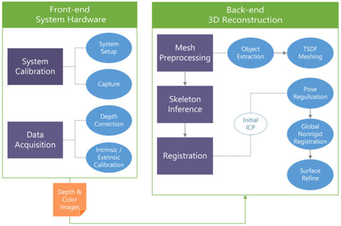
Our system (Figure 1) consists of two parts: the front end and the back end. In the front end, our hardware system design aims to maximize the depth map accuracy by analyzing the sensor noise pattern. This is done through system calibration, which includes an experiment to measure and model the sensor depth bias as a function of distance, and a standard sensor intrinsic and extrinsic calibration. In the back end, we propose a nonrigid registration framework that is appropriate for the semi-nonrigid pose assumption (i.e., various human body poses appear as a high degree of deformations around skeletal joints, whereas modest deformations appear around link segments). Partial scan meshes are reconstructed during mesh preprocessing. Then, skeletal joint positions are inferred through multimodality registration. With partial scan meshes and skeletal data, the body surface is reconstructed through our nonrigid registration framework.

FIGURE 1.

System overview. TSDF = truncated signed distance function; ICP = iterative closest point

4 ∣. SYSTEM HARDWARE

4.1 ∣. Data acquisition

4.1.1 ∣. System setup

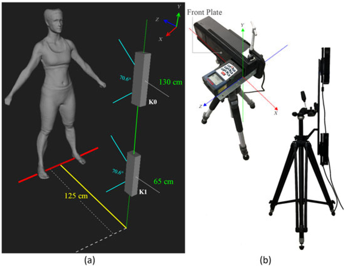
Our capture system consists of two Kinect v2 sensors, one 28” twin camera slide bar, and a tripod. The sensors are vertically mounted on the two ends of the slide bar to reach an optimal accuracy and capture volume. Figure 2 shows our capture system.

FIGURE 2.

System setup. (a) The setup of the two Kinects relative to the subject. The lower camera (denoted K1) was mounted at a height of 65 cm from the ground, and the upper camera (denoted K0) was mounted at a height of 130 cm from the ground. The distance from camera center to the subject is approximately 125 cm, and the camera vertical Field of View (FOV) is 70.6°. Using this configuration, the maximum allowable user height is 219 cm. (b) Left: hardware setup for depth bias analysis using a laser range instrument (e.g., Bosch^® laser measure). Right: hardware setup for capture, showing the two Kinects and the mounting frame

4.1.2 ∣. Capture

During the scan, the subject stands upright at approximately 125 cm from the sensors holding an “A pose” (Figure 2a), that is, arms open roughly 45° and feet open roughly 45 cm. The data acquisition takes eight scans (each corresponding to a pose) in total with the user rotating roughly 45° between each scan and holding the pose for approximately 1 s. Moreover, 30 frames of the depth image and 1 frame of the color image are collected for each scan.

4.2 ∣. System calibration

4.2.1 ∣. Depth correction

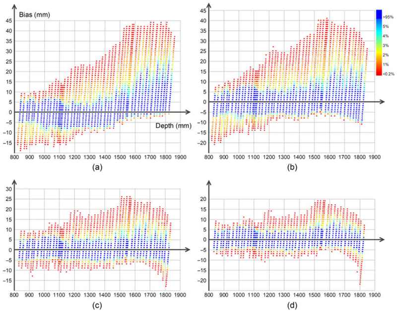
We designed an experiment to investigate the raw depth bias pattern of the Kinect using a 4.2 m × 3.2 m flat wall and high-precision distance-measuring instrument. We mounted a laser measure in front of and perpendicular to the sensor’s front plate (Figure 2b, left). The wall was perpendicular to the ground and large enough to cover the entire capture view at any sample distance. The x-z plane of Kinect Infrared (IR) sensor was calibrated to be parallel to the ground. We used laser distance measurements as ground truth, and a constant bias coefficient was calculated as the offset of the IR camera optical center to the Kinect’s front plate. The bias coefficient was experimentally measured by optimally matching the real and virtual corner-to-corner distance of corners randomly selected from a checkerboard. We took 50 uniform distance samples from 0.8 to 1.8 m with 3 captures for each sample and 30 frames per capture. For each capture, the sensor z-axis was adjusted to be perpendicular to the wall, and we repeated the capture process three times at each sample distance to mitigate the experimental error.

We modeled the depth bias pattern using quadratic regression and used it to correct the depth from the Kinect. As shown in Figure 3, we plotted the bias as a function of depth (Figure 3a) and compared three correction setups: global quadratic (Figure 3b), large patch regional quadratic with patch size of 48 × 48 pixels (Figure 3c), and small patch regional quadratic with patch size of 20 × 20 pixels (Figure 3d). Similar to the work of Dou et al.,³⁰ for each patch, we used 16-pixel overlap to increase the smoothness of correction. The majority bias (labeled in blue, covering more than 95% of the measure bias) was used for quadratic data fitting to rule out the impact of outliers. Our conclusion is that using regional quadratic regression to correct the depth bias works well at suppressing outliers, and the small patch correction outperforms the large one. In our implementation, we employed the regional quadratic regression with 20 × 20 patches for depth correction.

FIGURE 3.

Kinect bias pattern and depth correction. (a) Bias pattern as a function of depth. The majority bias distribution is in blue with appearance rate more than 95%. The other colors represent the minority bias distribution with appearance rate less than 5% and red one representing less than 0.02%. (b) Global quadratic correction. (c) Regional quadratic correction with 48 × 48 patch and an overlap of 16 pixels. (d) Regional quadratic correction with 20 × 20 patch and an overlap of 16 pixels

4.2.2 ∣. Intrinsic and extrinsic calibration

We used an 8 × 7 standard checkerboard pattern to calibrate the intrinsic parameters of the Kinect IR and RGB cameras and the extrinsic parameter from RGB to IR cameras. The multithread asynchronous data acquisition front end was developed based on the Libfreenect2 library.³¹

5. ∣. THE 3D RECONSTRUCTION

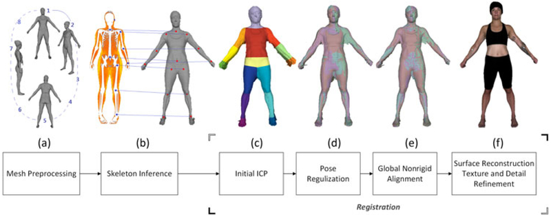
Figure 4 shows an overview of our approach, which consists of the following steps: (a) Mesh preprocessing (Figure 4a) generates eight high-resolution partial scan meshes from depth and color images captured in the front end. (b) Skeleton inference (Figure 4b) infers skeletal joint positions by multimodality registration. (c) Registration (Figure 4c-f) reconstructs the 3D body surface using nonrigid registration. Our nonrigid registration framework has the following substeps: First, we initially align partial meshes with rigid ICP and divide each partial scan mesh into 15 segments according to the joint positions (Figure 4c). Second, we regularize poses by deforming partial scan meshes under the articulated motion constraint and the global loop closure constraint (Figure 4d). Third, we perform a global nonrigid registration to stitch the meshes further and generate a watertight surface (Figure 4e). Fourth, we map high-frequency details and texture to the watertight surface (Figure 4f).

FIGURE 4.

Reconstruction pipeline. ICP = iterative closest point

5.1 ∣. Mesh preprocessing

Eight partial scan meshes are generated in this step corresponding to the eight poses. To generate the partial scan meshes efficiently and accurately, we first reconstruct low-resolution meshes from the two cameras to obtain an optimal extrinsic transformation. Then, we generate a high-resolution partial mesh by fusing two cameras’ depth images with the optimal extrinsic transformation. An adaptive size truncated signed distance function (TSDF) volume (i.e., the size of volume fits the bounding box of the scanned subject) is employed to optimize the memory and computational efficiency, as well as to average out the random sensor noise. The partial meshes are extracted from the TSDF volume using marching cubes.³² To clip the ground, one extra scan without a subject is taken to estimate the ground plane parameters during preprocessing.

5.2 ∣. Skeleton inference

Accurate skeletal joints inference is critical, as our reconstruction method relies heavily on the articulated motion assumption. Unlike the methods of Wang et al.⁸ or Cui et al.,³ we infer skeletal joints from personalized body composition scans. In our study, we have access to the body composition image from DEXA for each tested subject (Figure 5b). We propose a novel approach to accurately infer skeletal joint positions from DEXA images through multimodality registration. Furthermore, for scans without available DEXA references, we present a supervised learning model to predict joint locations. To the best of our knowledge, this is the first attempt to utilize registered medical imaging as the reference to infer skeletal joints in a 3D body reconstruction system. Using this approach, a high degree of accuracy for skeletal joints inference and body segmentation can be achieved. This model is also capable of predicting body composition map without the use of subject-specific DEXA scans, which is itself a useful tool.

FIGURE 5.

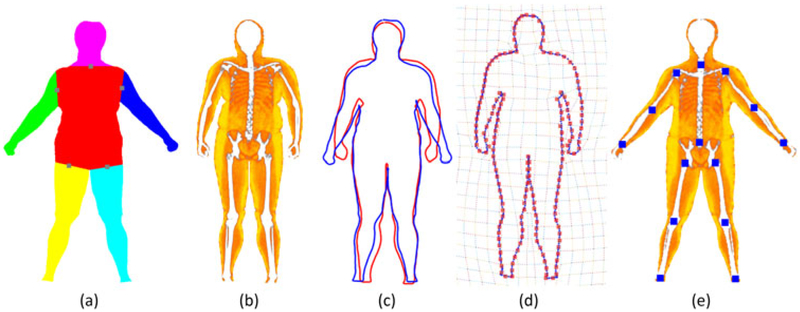
Multimodality registration for mapping skeletal joints. (a) Input shape with binary classified body segments and their rotation center (gray points). (b) Target shape from DEXA scan. (c) Silhouette of the source shape after pose regularization (blue) and silhouette of the target shape (red). (d) Free-form deformation-based shape registration. (e) Skeletal joints and body composition mapping from the target shape to the original source shape

5.2.1 ∣. Shape registration framework

To map the data from one modality to the other, the key is to establish correspondences between the shapes. Our registration framework consists of two steps: pose regularization and nonrigid registration. Without loss of generality, we define the source and target shapes in the form of 2D triangle mesh as $\mathcal{S}$ and $\mathcal{T}$, respectively, from which we sample ordered boundary vertex sets ${\mathcal{S}}_b$ and ${\mathcal{T}}_b$.

Pose regularization.

First, we classify the vertices on source shape $\mathcal{S}$ into six body segments—torso, head, left arm, right arm, left leg, and right leg—as color coded in Figure 5a. The rotation center of each segment is heuristically defined, represented as gray points in Figure 5a. Next, we calculate an affine transformation matrix for each segment on source shape $\mathcal{S}$ to roughly match the pose of target shape $\mathcal{T}$. Finally, vertices on source shape S are transformed as a weighted blend of the segment’s affine transformations. $\tilde{\mathcal{S}}$ denotes the source shape after pose regularization, and its boundary is denoted by ${\tilde{\mathcal{S}}}_b$.

Nonrigid registration.

To further align source shape $\tilde{\mathcal{S}}$ to the target, we adopt the method of Rouhani et al.,³³ a robust shape registration framework that exploits local curvature features. The deformation is parameterized by free-form deformation (FFD), where P denotes the control lattice.

In shape registration, the goal is to minimize the distance between shape correspondences while deforming the source shape as smoothly as possible (1). The smoothness term E_smooth encourages the integral of the second-order derivatives of the linear functions to be small. The data term E_data (2) interpolates between two types of error metrics: point-to-point and point-to-plane. The interpolation weight W (3) is proportional to the local curvature κ. For target geometry with salient curvatures, point-to-point error metric dominates the penalty term to encourage a localized correspondence search. For target geometry with low curvature, point-to-plane error metric dominates the penalty term to allow the correspondence search to “slide over” target ${\mathcal{T}}_b$ to avoid being trapped in local minima.³⁴

$${\mathbf{P}}^{\ast }=\underset{\mathbf{P}}{\text{argmin}}\sum E_{\text{data}}(\tilde{v}\in FFD({\tilde{\mathcal{S}}}_b),t\in {\mathcal{T}}_b)+\lambda E_{\text{smooth}}(\mathbf{P})$$ (1)

$$E_{\text{data}}(\tilde{\mathit{v}},\mathit{t})=W{\Vert (\tilde{\mathit{v}}-\mathit{t})\cdot {\mathbf{T}}_t\Vert }_2^2+{\Vert (\tilde{\mathit{v}}-\mathit{t})\cdot {\mathbf{N}}_t\Vert }_2^2$$ (2)

$$W=1+\frac{1}{\kappa \ast signed\_dis(\tilde{\mathit{v}},\mathit{t})-1}.$$ (3)

The shape registration is performed in a nonrigid ICP fashion. For each step, the corresponding pairs $\tilde{\mathit{v}}\in FFD({\tilde{\mathcal{S}}}_b)$, $\mathit{t}\in {\mathcal{T}}_b$ are updated with the latest deformation parameter P. The stiffness λ is set to be high at the start of iteration to enforce a global alignment and gradually relaxed to encourage local deformation. Rouhani et al.³³ formulated an elegant quadratic objective function with respect to the deformation parameter P, resulting in a closed-form solution for each ICP iteration. Let P_conv denote the final deformation parameter and ${\tilde{\mathcal{S}}}_b^{\mathcal{T}}$ denote the boundary shape at convergence (Figures 5d and 7c). Shape $\tilde{\mathcal{S}}$ is then deformed to ${\tilde{\mathcal{S}}}^{\mathcal{T}}$ with deformation parameter P_conv.

FIGURE 7.

Skeletal joints and body composition inference via supervised learning. (a) Training shapes in dashed line, color coded with body mass index (BMI). The average of training shapes outlined in black. (b) The shape to be predicted. (c) Shape processing: register the template to the predicting shape. (d) Shape prediction: predict the best-matched shape (light blue) for the predicting shape (red). (e) Skeletal joints and body composition mapping

5.2.2 ∣. Skeletal joints inference via multimodality registration

We select the first and the fifth partial scan meshes for skeletal joints inference, corresponding to poses that face forward and backward relative to the cameras. To simplify the notation, we take the first partial scan mesh as an example. The process is analogous to the fifth. We define the source shape $\mathcal{S}$ to be the 2D orthogonal projection of the first mesh. The DEXA image is converted into 2D mesh labeled with skeletal joints, corresponding to the target shape $\mathcal{T}$. We first regularize the pose of source shape $\mathcal{S}$ to match the pose of target shape $\mathcal{T}$, yielding regularized shape $\tilde{\mathcal{S}}$ and its corresponding boundary ${\tilde{\mathcal{S}}}_b$ (Figure 5c). In our experiment, in most cases, the source shape $\mathcal{S}$ is capable of being registered to the target $\mathcal{T}$ without pose regularization. However, with a prior knowledge of the shape’s underlying structure, we initially regularize the pose to avoid undesirable distortion and hence to increase the registration accuracy and stability. After pose regularization, the source boundary ${\tilde{\mathcal{S}}}_b$ is registered to the target boundary ${\tilde{\mathcal{T}}}_b$ by solving the objective function in Equation 1 iteratively (Figure 5d). Source shape $\tilde{\mathcal{S}}$ is then deformed via FFD with the optimal deformation parameters, resulting in the aligned shape ${\tilde{\mathcal{S}}}^{\mathcal{T}}$. The skeletal joints labeled on target mesh $\mathcal{T}$ is then mapped to the aligned shape ${\tilde{\mathcal{S}}}^{\mathcal{T}}$ and thus to the 2D orthogonal projection shape $\mathcal{S}$ (Figure 5e). Finally, the skeletal joints are inferred on the partial scan mesh.

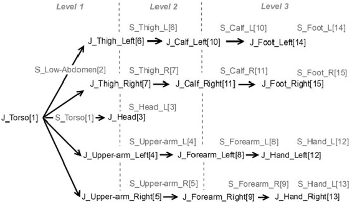
We initially align all the partial scan meshes through global rigid ICP registration. Based on mapped joints, we segment the first and the fifth partial scan meshes into 15 segments as illustrated in Figure 8 and propagate the joints and segmentations throughout the rest of partial scan meshes.

FIGURE 8.

Skeleton hierarchy. J stands for the joint, and S stands for the segment, followed by the name of each joint or segment. The index after a name is the order of this joint or segment in the list

5.2.3 ∣. Skeletal joints inference via supervised learning

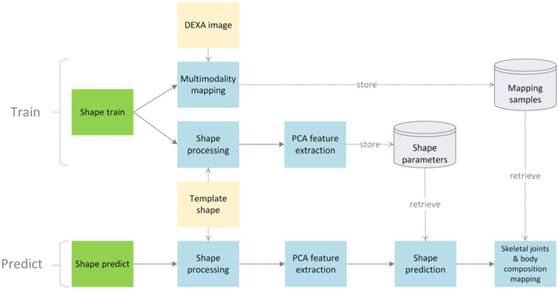
We further developed a novel predictive model through supervised learning to infer skeletal joints and body composition for arbitrary subjects without the need for DEXA scans. Our approach consists of a training phase and a predicting phase (Figure 6).

FIGURE 6.

Flowchart of skeletal joints and body composition inference via supervised learning showing training phase (top) and predicting phase (bottom). PCA = principal component analysis

In the training phase, we take various body shapes and corresponding DEXA images as input. For each training shape, we infer skeletal joints and body composition map from the DEXA image by multimodality registration (Figure 6, Multimodality mapping). Textured training shapes are stored in mapping sample database (Figure 6, Mapping samples). A uniform template is registered to each of the training shapes via shape registration (Figures 6, Shape processing, and 7a). Then, we analyze the variation of registered templates using principal component analysis (PCA) and extract the top three PCA components as the basis for the feature space. Shape features for each training shape are calculated as the projection of corresponding registered template on the PCA feature space (Figure 6, PCA feature extraction). Shape features are stored in shape parameter database (Figure 6, Shape parameters).

In the predicting phase, we adopt a nonparametric regression predictive model to predict skeletal joints and body composition map for new shapes (Figure 7b), including but not limited to shapes generated from partial scan meshes. First, we register the template shape to the new shape via shape registration (Figures 6, Shape processing, and 7c). The PCA features are extracted for the new shape by projecting the aligned template onto the PCA feature space (Figure 6, PCA feature extraction). One best-matched shape is predicted by searching for the training shape whose PCA features have the minimum Euclidean distance total the new shape’s features (Figures 6, Shape prediction, and 7d). Finally, we register the best-matched shape to the new shape to map the skeletal joints and body composition map (Figures 6, Skeletal joints & body composition mapping, and 7e).

5.3 ∣. Surface reconstruction

To reconstruct the 3D human body, our solution integrates the articulation constraint and the global loop closure constraint into the as-rigid-as-possible nonrigid registration framework. The articulation constraint prevents connected segments from drifting apart during registration. The segmentwise global loop closure constraint ensures that the registration error distributes evenly throughout the partial scans. This prevents alignments from falling into the local minima and hence enhances the registration quality where occlusions exist. The as-rigid-as-possible deformation framework models an effective way to simulate the skin deformation under articulated motion, preventing mesh near joints from unnatural folding or stretching during registration.

In the rest of the paper, we represent the globally aligned partial scan mesh in pose i as $M_i=\{v_i^k\in {\mathbb{R}}^3,k=1,\dots ,n\}$, i = 1, … , 8, where n denotes the number of vertices in the mesh. We represent the embedded deformation graph of M_i as $E{D}_i=\{g_i^k\in {\mathbb{R}}^3,k=1,\dots ,m\}$, i = 1, … , 8, where m denotes the number of nodes in the graph. Vertices on each partial mesh are classified into 15 segments, where $S_i^k$ denotes the kth segment of partial mesh M_i. Segments of eight partial meshes share one set of joints, whose positions are denoted by $\mathit{J}=\{{\mathit{J}}_k\in {\mathbb{R}}^3,k=1,\dots ,15\}$. We assign to each segment $S_i^k$ a rigid transformation $\mathit{T}{\mathit{r}}_i^k=\{({\mathit{R}}_i^k{\mathit{t}}_i^k),\mid {\mathit{R}}_i^k\in SO(3),{\mathit{t}}_i^k\in {\mathbb{R}}^3\}$. Figure 8 lists the joints and segment indices and their hierarchy.

The basic deformation model.

Our nonrigid registration framework is based on the embedded deformation model of Sumner et al.²⁶ The deformation of the partial mesh M_i is abstracted to the deformation of the embedded graph ED_i, where the transformation of each graph node in ED_i is constrained to be as rigid as possible. We propose to generate the embedded graph through a multiresolution k-nearest neighbor (k-NN) method to establish fast and effective connections between random sample points.

The transformation parameters of graph nodes are calculated by minimizing the energy function E described in Equation 4, as follows:

$$E={\mathrm{w}}_r{E}_{\text{rigid}}+{\mathrm{w}}_s{E}_{\text{smooth}}+{\mathrm{w}}_c{E}_{\text{corr}}.$$ (4)

Two constraints are imposed to formulate the properties of deformation. The rigidity term $E_{\text{rigid}}={\sum }_{i=1}^{m}Rot({\mathit{R}}_i)$ enforces rotation matrix R associated with each graph node to be as orthogonal as possible, where the Rot(R) reflects the orthogonality of matrix R. The smoothness term $E_{\text{smooth}}={\sum }_{i=1}^m{\sum }_{k\in \mathcal{N}(i)}\Vert {\mathit{R}}_i\cdot (g^k-g^i)+g^i+t_i-(g^k+t_k){\Vert }_2^2$ enforces the transformation of each node to be consistent with its neighbors', where $\mathcal{N}(\cdot )$ represents neighbor nodes that connect to the graph node. The correspondence term E_corr enforces the distance error of correspondences to be small, which will be formulated differently in different registration phases.

5.3.1 ∣. Pose regularization

In this phase, we aim to initially align eight partial meshes through the as-rigid-as-possible deformation framework under the articulated motion constraint and the global loop closure constraint.

Joint constraint.

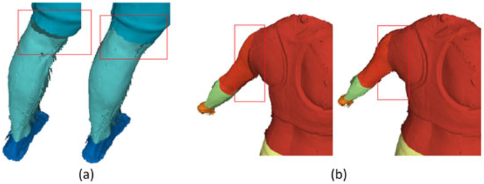
A joint constraint prevents the common ends of two connected segments from drifting apart after the transformation. We adopt the soft ball joint constraint method of Knoop et al.³⁵ to proportionally add artificial joint-to-joint correspondences into the segmentwise registration. The ratio of artificial to total correspondences is treated as a weight of this joint constraint. Figure 9 shows a comparison of segmentwise global rigid registration with and without the joint constraint. Segments tend to drift away (Figure 9a,b left) without a soft joint constraint.

FIGURE 9.

The joint constraints comparison. (a) Left: without the knee joint constraint. Right: with the knee joint constraint. (b) Left: without the shoulder joint constraint. Right: with the shoulder joint constraint

Global loop closure constraint.

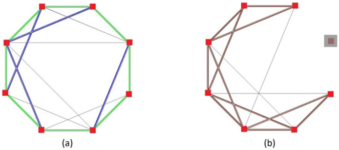
During pose regularization, we treat segments of partial scans as moving rigidly and the shape change as negligible. For each segment S, we globally align all eight partial segments S^k, k = 1, … , 8 under the global loop closure constraint and the soft joint constraint. In practice, we cannot always guarantee a complete loop (i.e., each node connects to its two adjacent nodes in the graph) due to occlusion, especially in areas such as inner sides of upper arms or thighs. Therefore, for each of these types of segments, we perform the explicit loop closure constraint (Figure 10b). For each of the rest, we perform the more flexible implicit loop closure constraint (Figure 10a). The explicit constraint predefines which pair of meshes should be aligned. The implicit constraint determines whether to align the mesh pair or not based on whether the overlapping area of the pair is larger than a certain threshold. After aligning each selected pair of meshes, we then globally distribute the alignment error throughout the graph (Figure 10).

FIGURE 10.

Examples of implicit graph (a) and explicit graph (b). The red dots represent mesh nodes, and the gray lines denote all candidate edges. Mesh nodes connected by lines can be registered. In the implicit graph, the green highlight edges represent the predefined baseline edges for the loop and, the blue highlight edges are selected from the rest of the edges (gray lines) based on an implicit threshold. The implicit threshold is set as the minimum overlap area of the mesh pair on baseline edges. In the explicit graph, the brown highlight edges represent the explicitly predefined edges, which are mandatorily computed during registration. The node covered by the gray square represents missing mesh due to occlusion

The correspondence term.

Eight partial scan meshes are deformed, guided by the outputs of the segmentwise articulated global registration under the above two constraints. We specify the correspondence term for pose regularization in Equation 5, where T(g_i, Tr) transforms embedded graph node g_i with the transformation matrix Tr of the segment that g_i belongs to.

$$E_{\text{corr}}=\sum _{i=1}^m{\Vert g_i-T(g_i,\mathit{Tr}[segmet\_id(g_i)])\Vert }_2^2.$$ (5)

Implementation.

First, we perform a segmentwise articulated global registration to align all segments. We take segments of partial scans $S_i^k$, i = 1, … , 8, k = 1, … , 15 and the joint positions J_k, k = 1,… , 15 as inputs. We initially set the transformation matrix Tr for each segment of partial scans to identity. The segmentwise registration is performed in a top-down fashion from level 1 to 3 (Figure 8). Segments belonging to level l (l = 1, 2, 3) are aligned under the constraints. The transformation matrices and joint positions are updated accordingly and then propagated to their descendants. The outputs are the rigid transformation matrix Tr for each segment and updated joint positions. Second, eight partial meshes are deformed nonrigidly, guided by previous outputs. The correspondence is defined for each graph node according to the transformation of the segment this node belongs to. During the optimization, we minimize Equation 4 with a correspondence term specified in Equation 5 to get the deformation parameter for each graph node. The partial scan meshes M_i, i = 1,… ,8 are then deformed by their corresponding embedded deformation graphs. We represent the pose regularized partial scan meshes as RM_i, i = 1, … ,8.

5.3.2 ∣. Global nonrigid registration

After pose regularization, the eight meshes RM_i, i = 1,… ,8, are close enough to be further registered. We adopt the global nonrigid registration framework of Li et al.⁵ First, each mesh is pairwisely registered to define global correspondences. Then, with the correspondences, eight meshes are stitched through global nonrigid registration.

Pairwise nonrigid registration.

To pairwisely align partial scan meshes, the point-to-point and point-to-plane error metrics are adopted for the correspondence constraint (6). Our pairwise alignment suffers less from local minima due to the pose regularization.

$$E_{\text{corr}}=\sum _{(\tilde{\mathit{v}},\tilde{t})\in {\mathrm{C}}_{\text{pairwise}}}\Vert \tilde{\mathit{v}}-\tilde{\mathit{t}}{\Vert }_2^2+{\Vert (\tilde{\mathit{v}}-\tilde{\mathit{t}})\cdot {\mathit{N}}_{\tilde{t}}\Vert }_2^2.$$ (6)

Global nonrigid registration.

The global alignment aims to stitch the eight meshes simultaneously. We predefine global correspondences using pairwise nonrigid registration and then solve for deformation parameters of the eight embedded graphs in one optimization. The correspondence constraint for global nonrigid registration (7) enforces the point-to-point distances of global correspondence pairs $(\tilde{\mathit{v}},\tilde{\mathit{t}})\in {\mathrm{C}}_{\text{global}}$ to be small.

$$E_{\text{corr}}=\sum _{(\tilde{\mathit{v}},\tilde{t})\in {\mathrm{C}}_{\text{global}}}\Vert \tilde{\mathit{v}}-\tilde{\mathit{t}}{\Vert }_2^2.$$ (7)

Implementation.

The first step is to define global correspondences by pairwisely deforming RM_i to its next neighbor RM_i+1 (the last mesh deforming to RM₁). For each pair after registration, we uniformly sample the source mesh, and for each sample point, we search for its correspondence on the target based on the Euclidean distance and normal compatibility. Indexes of sample points and their correspondences are stored in the global correspondence table GC_i(i = 1, … ,8). The second step is to globally register the eight regularized partial meshes RM_i (i = 1, … ,8) based on the global correspondences defined in the previous step. The global correspondence tables for the eight meshes are merged into one table GC so that samples on RM_i have bidirectional correspondence on both RM_i−1 and RM_i+1. After optimization, the outputs are the eight globally aligned partial meshes GRM_i(i = 1,… ,8). In the third step, we merge these eight globally aligned partial meshes to generate a watertight surface $\mathcal{L}$ through Poisson reconstruction.¹³

5.3.3 ∣. Detail Mapping and Texture Refinement

Detail mapping.

The Poisson reconstruction¹³ tends to oversmooth the high-frequency details of the original meshes GRM_i(i = 1,… ,8). We propose to map high-frequency details from the globally aligned partial meshes to surface $\mathcal{L}$. We nonrigidly deform the aligned partial meshes toward the watertight surface $\mathcal{L}$ and optimize per-vertex correspondence of $\mathcal{L}$ to each mesh. After convergence, we warp the vertices on surface $\mathcal{L}$ toward the latest correspondences with a Laplacian smoothness constraint. With the correspondences, we also preliminarily map the texture onto the watertight surface $\mathcal{L}$.

Texture refinement.

Because our goal is to develop a consumer system for high-quality 3D human body modeling, we do not have strict illumination requirements. However, texture artifacts occur due to color inconsistencies. We employed a diffusion method to mitigate texture artifacts caused by illumination variance, that is, nonuniform lighting. The diffusivity is determined by the color similarity of a given vertex and its k-NN vertices to preserve edge details but, at the same time, smooth out color inconsistency artifacts. Additionally, the facial detail is enhanced by a geometry and texture supersampling.

6 ∣. EXPERIMENT

6.1 ∣. Data collection

We have conducted a threefold experiment to collect DEXA scan images, to test the robustness of our body scan system, and to verify reconstruction accuracy and reliability.

The experiment has a sample size of 28 subjects (14 males and 14 females). This is considerably larger than the sample size reported in similar studies.^36,37 We consider the sample size to be sufficient if the width of the 95% confidence interval is at most 1.5% of the value to be estimated. We demonstrate this in the results section. This experiment is the first phase accuracy study of a larger experiment consisting of 160 subjects that we are conducting to calculate the percentage of body fat using surface scans. The data collection involving human subjects was approved by the Institutional Review Board (IRB).

The subjects were recruited from the Washington, DC, metro area, with age of 25.7 ± 5.1 and BMI of 23.3 ± 3.1. We drew 34 landmarks on each subject corresponding to anatomic definitions of chest, waist, abdomen, hip, thigh, calf, shoulder, elbow, wrist, patella, and ankle. Two landmarks (for measurements on arms and legs) and four landmarks (for measurements on torso) were placed in each location as a reference for the caliper and tape measurements. The test took 1 h for each subject, including the DEXA scan, the scan using our system, and the caliper and tape measurements.

Scan with the system.

Subjects were asked to change into a tight-fitting uniform including sleeveless compression tops (for males), sports bras (for females), swimming shorts, and swimming caps. The landmarks were drawn before the scan. Each subject was scanned three times. The textured 3D body shapes were reconstructed afterward with all landmarks visible on the virtual models. Euclidean distance between markers on 3D virtual models was calculated and recorded.

Manual measurements.

We measured the point-to-point linear distance between landmarks with a caliper and the length of arms and legs with a tape measure. Two measurements were taken to mitigate measurement error. During the measurement, subjects held approximately the same pose as they did during the scan. Our accuracy comparison is in between the manual caliper/tape measure on real subjects and the vertex-to-vertex Euclidean distance measure on reconstructed virtual 3D models.

6.2 ∣. Surface reconstruction

During mesh preprocessing, we reconstructed multiresolution partial scan meshes from depth and color images using the TSDF fusion¹⁷ and the marching cubes³² algorithms. The coarse mesh was reconstructed at a resolution of 192 voxels/m, and the fine mesh was reconstructed at a resolution of 384 voxels/m. The implementations were based on the Kangaroo Library.³⁸

In shape nonrigid registration, we set the FFD control lattice to be 30 × 30, covering a unit deformation space, that is, [0,1]². Shapes were rescaled uniformly to fit into the unit square before registration. We initialized the stiffness λ to 10⁵, and for each iteration, we reduced λ by 25% until convergence.

We implemented the segmentwise articulated global rigid registration based on the VCG Library.³⁹ We experimentally set the weight for articulation constraint to 0.1 and the overlapping area threshold for the implicit graph to 0.2.

Our surface reconstruction framework is based on the as-rigid-as-possible deformation model. The deformation graph node was connected by its k-NN. We set k to 10 for all embedded deformation graphs during registration. The optimization function consists of three energy terms: the rigid term, the smoothness term, and the correspondence term. The corresponding weights are denoted by w_r, w_s and w_c. For pose regularization, we experimentally set w_r to 100, w_s to 10, and w_c to 5. For pairwise nonrigid registration and detail mapping, we experimentally set w_r to 10, w_s to 5, and w_c to 1. For each iteration, we reduced w_r by half. For global nonrigid registration, we experimentally set w_r to 50, w_s to 2.5, and w_c to 1. For each iteration, we solved the nonlinear objective function using the Gauss–Newton method, where the Cholesky decomposition was solved with the CUDA conjugate gradient solver.⁴⁰

Our reconstruction system is able to run on average commodity hardware. In our experiment, we used Intel^® Core i7–4790 CPU with 32GB RAM and an NVIDIA^® GeForce GTX 750 GPU with 2GB DRAM to process the data. The processing times for each step are illustrated in Table 1.

TABLE 1.

Processing time for one instance of reconstruction

	Meshing	Skeleton mapping	Pose regularization	Pairwise nonrigid	Global nonrigid	Poisson reconstruction	Texture
Time (s)	391.47	108.37	384.71	210.36	170.22	49.15	224.47

7 ∣. RESULTS

7.1 ∣. Skeleton inference

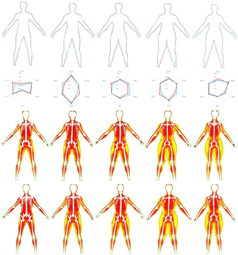
We conducted a holdout validation test to evaluate the accuracy of our predictive model for skeletal joints and body composition inference. The model was trained using body shapes with various body sizes (Figure 7a). The validation test consists of new shapes and their DEXA images. Five inference results generated via our predictive model are illustrated in Figure 11, row 3. In the predictive model, we extracted PCA features of the input shape and predicted the best-matched shape from the training shape dataset. Five test shapes and their best-matched shapes are illustrated in Figure 11, row 1. Corresponding PCA features are visualized in radar plots in Figure 11, row 2. The test ground truth was generated by directly mapping the DEXA image to the test shape through multimodality registration (Figure 11, row 4). Based on a training sample size of 12, the mean error of skeletal joints prediction is 1.63 cm and the mean accuracy of body composition prediction is 82.87% (Table 2).

FIGURE 11.

Holdout validation for skeletal joints inference via supervised learning. (Row 1) Body shape prediction. The best-matched shape (light blue) is predicted for each test shape (red). (Row 2) Radar plots of six PCA features (i.e., PCA1_X, PCA2_X, PCA3_X, PCA1_Y, PCA2_Y, and PCA3_Y) for the five test shapes (red) and their corresponding predicted best-matched shapes (light blue). (Row 3) Predicted skeletal joints and body composition. (Row 4) Test ground truth. Skeletal joints are represented as blue squares. For body composition, white denotes bones, red denotes muscles, and yellow denotes fat. Shape boundary is colored in green

TABLE 2.

Skeletal joints prediction error and body composition prediction accuracy

	Test 1	Test 2	Test 3	Test 4	Test 5	Mean
Skeletal joints error (cm)	1.49	1.41	1.23	2.57	1.45	1.63
Body composition accuracy	82.01%	82.79%	82.69%	84.31%	82.53%	82.87%

7.2 ∣. Surface reconstruction

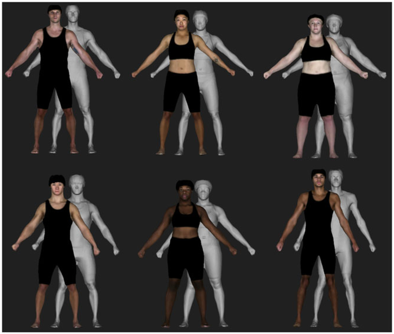
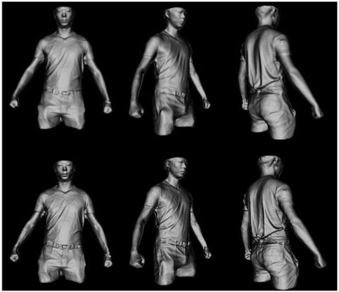
Figure 12 shows our reconstruction results. Our system is also capable of capturing complex surfaces for general-purpose 3D scan and reconstruction such as the case in which the subjects wear loose clothes. The surface details were reconstructed by mapping high-frequency geometry details from the deformed partial meshes to the oversmoothed watertight surface generated by Poisson reconstruction.¹³ In Figure 13, details of the T-shirt and pants, wrinkles, face, hair, and ears are shown.

FIGURE 12.

Reconstruction results

FIGURE 13.

Comparison of detail mapping. Top: the watertight surface generated by Poisson reconstruction. Bottom: the detail refined mesh

7.3 ∣. Accuracy evaluation

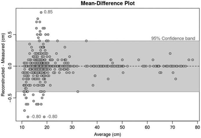
We obtained 24 measurements on each of the 28 subjects and summarized them as a mean-difference plot in Figure 14. The vertical axis is the difference between the value obtained from the 3D reconstruction and that obtained by tape measure or caliper. The horizontal axis is the average of the virtual and real (caliper or tape) measure. A 95% confidence band (−0.4 cm to 0.4 cm) is superimposed on the plot for reference. Most (97.4%) measurements are within 5 mm of each other, with the largest discrepancies being 0.85 cm and −0.80 cm. Note that the caliper and tape measurements also involve some error.

FIGURE 14.

Mean-different plot of the overall discrepancies

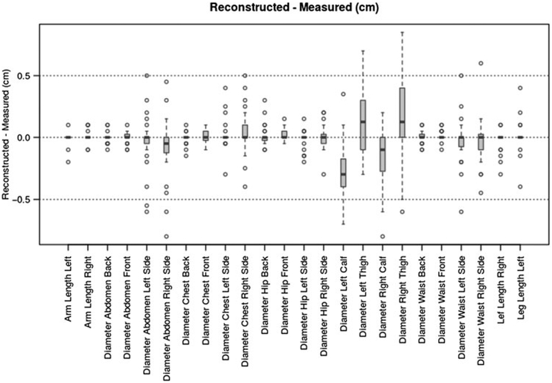
Figure 15 breaks down the discrepancies by location and displays boxplots of the differences between 3D reconstructed and manually measured values. As noted above, the reconstructed and measured values are, for the most part, within 5 mm of each other. Most discrepancies are in the abdomen, calf, and thigh measurements and appear to be due in part to difficulties in performing the manual measurements and in part to the registration and sensor intrinsic errors. The 95% confidence accuracy interval for each of the 24 measurements was calculated. With the sample size of 28, the worst-case interval width was 0.27 cm, and the worst-case relative error was 1.5%.

FIGURE 15.

Discrepancies by location

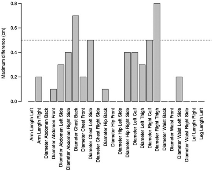
Finally, as a test of the repeatability of the reconstruction, all 24 measurements for the first subject were repeated 3 times. The intraclass correlation between measurements was 0.99990, with a 95% confidence interval of (0.99981, 0.99996). The worst error at each location was calculated as the largest of the three values minus the smallest. These worst errors are shown in Figure 16. We hypothesize that the errors are mainly due to a combination of pose change, shifting clothing, and breathing between data taking.

FIGURE 16.

Maximum difference of repeated reconstructions

In Table 3, we compare our body reconstruction geometry accuracy and whole-body volume accuracy with state-of-the-art body reconstruction systems that are widely used in academic research and commercial applications. Rigorous scientific validations have been conducted for 3dMDface^® by Aldridge et al.³⁶ with 15 subjects and for Crisalix 3D^® by de Heras Ciechomski et al.³⁷ with 11 subjects. Li et al.⁵ validated their algorithm using one rigid mannequin and compared their reconstruction result with the ground truth from the laser scanner. Zhang et al.¹⁰ validated their method with one articulated rigid mannequin, also taking laser scan as the ground truth. We do not have the details of the accuracy claims of the other systems. The result shows that our reconstruction system geometry accuracy is superior to Crisalix 3D^® and Styku^® for torso region and to methods of Li et al. and Zhang et al. for the whole-body areas. The volume accuracy outperforms high-end body scanner Telmat SYMCAD^®.

TABLE 3.

Comparison of geometry and volume accuracy with state-of-the-art body reconstruction systems

System for body reconstruction	Techniques	Cost	Source	Experiment data source	Experiment details	Region	Geometry error (mm)	Volume error
3dMDface®	Stereo-photogrammetry	$$$$$$	36	Experiment with real subjects	N = 15, L = 20, M = 14	Face	1.263
3dMDbody®	Stereo-photogrammetry	$$$$$$	41	No detail		Body	0.2–1
TC2 NX-16®	Structured white light	$$$$$	42	Factory tech specs		Body	<1
Telmat SYMCAD®	Structured white light	$$$$$	43	No detail		Body	<1	−8%
Crisalix 3D ®	Image-based reconstruction	$$$$	37	Experiment with real subjects	N = 11, L = 14	Torso	2–5
Styku®	KinectFusion	$$$	44	Factory tech specs		Torso	2.5–5
Li et al.	Kinect nonrigid	$$$	5	Rigid mannequin	N = 1	Body	3
Zhang et al.	Kinect nonrigid	$$$	10	Articulated rigid mannequin	N = 1	Body	2.45
Ours	Kinect nonrigid	$$$		Experiment withreal subjects	N = 28, L = 34, M = 24	Body Torso	2.048 1.717	3.63%

Note. N denotes the sample size of validation experiment, L denotes the number of landmarks, and M denotes the number of measurements collected per trial. The geometry error is compared in root mean square, except for the works of Li et al. and Zhang et al. (mean error). The volume error is compared in mean absolute difference.

8 ∣. CONCLUSION

In this paper, we present a high-quality and highly accurate 3D human body reconstruction system using commodity RGB-D cameras. Our registration framework integrates articulated motion assumption and global loop closure constraint to the as-rigid-as-possible deformation model to initially regularize partial scan meshes. By regularizing the pose, we achieve a relatively good initial condition for global nonrigid registration. Additionally, we investigated the depth sensor noise pattern with a rigorous experiment. We analyzed the noise pattern to correct the depth bias and to guide our hardware system design.

We designed and conducted a rigorous accuracy validation test for the proposed nonrigid human body reconstruction system. Our results show excellent agreement between the measurements obtained from the 3D reconstruction and those obtained manually, with a root mean square difference of 2.048 mm.

The multimodality skeleton mapping maximizes the segmentation accuracy. To the best of our knowledge, this is the first work that attempts to improve the skeletal joints inference accuracy for body scanner using multimodality registration. Moreover, the innovative supervised predictive model for skeletal joints inference makes it possible to extend the high-accuracy segmentation to arbitrary subjects independent from anatomical data, such as the DEXA image. Last but not the least, our predictive model is capable of predicting body composition map, that is, fat, muscle, and bone distribution, for various body shapes with a promising accuracy of 82.87% using a rather small training sample size of 12.

In the future, we are planning to develop the body composition predictive model to incorporate features such as weight, height, BMI, ethnicity, and geometric shape descriptors. We will develop a more comprehensive training sample set to cover a large variety of body shapes and demographic data. We foresee that the sophisticated predictive model will result in an enhancement of inference accuracy. The current multimodality registration and skeletal joints inference via supervised learning predict projected 2D body composition maps from 3D surface scans much like the results of DEXA scans. We are working to extend this algorithm to predict 3D body composition maps from 3D surface scans, which would have far-reaching implications for treating obesity.

Biography

Yao Lu is currently a Ph.D. candidate at The George Washington University, Department of Computer Science. She received the B.S. degree in Electrical Engineering from Communication University of China, China, in 2012 and M.S. degree in Computer Science from The George Washington University, USA, in 2014. Her research focuses on 3D surface reconstruction, nonrigid registration, and machine learning.

Shang Zhao is a doctoral student at The George Washington University department of computer science since 2015. He received the B.S. degree in Computer Science from Southwest University, China, in 2013 and M.S. degree in Computer Science from The George Washington University, USA, in 2015. His research domain of interest includes computer graph qics, virtual reality, motion tracking, medical simulation, and visualization.

Naji Younes is currently an associate professor in the Department of Epidemiology and Biostatistics at The George Washington University. He has over 20 years of experience designing, conducting, and analyzing clinical trials. His training and interests are both in mathematical statistics and software engineering, and he has been actively involved in the design and deployment of data management and reporting systems for clinical trials.

James K. Hahn is currently a professor in the Department of Computer Science with a joint appointment in the School of Medicine and Health Sciences at The George Washington University where he has been a faculty since 1989. He is the former chair of the Department of Computer Science. He is the founding director of the Institute for Biomedical Engineering and the Institute for Computer Graphics. His areas of interests are medical simulation, image-guided surgery, medical informatics, visualization, and computer animation. He has over 25 years of experience in leading multidisciplinary teams involving scientists, engineers, and medical professionals. His research has been funded by NIH, NSF, ONR, NRL, NASA, and a number of high-tech biomedical companies. He received his Ph.D. in Computer and Information Science from the Ohio State University in 1989.