

Abstract
PM2.5, or fine particulate matter, is a category of air pollutant consisting of particles with effective aerodynamic diameter equal to or less than 2.5 μm. These particles have been linked to human health impacts as well as regional haze, visibility, and climate change issues. Due to cost and space restrictions, the U.S. Environmental Protection Agency monitoring network remains spatially sparse. To increase the spatial resolution of monitoring, previous studies have used satellite data to estimate ground‐level PM concentrations, despite these estimates being associated with moderate to large uncertainties when relating a column measure of aerosol (aerosol optical depth) with surface measurements. To this end, we discuss a low‐cost air quality monitor (LCAQM) network deployed in California. In this study, we present an application of LCAQM and satellite data for quantifying the impact of wildfires in California during October 2017. The impacts of fires on PM2.5 concentration at varying temporal (hourly, daily, and weekly) and spatial (local to regional) scales have been evaluated. Comparison between low‐cost air quality sensors and reference‐grade air quality instruments shows expected performance with moderate to high uncertainties. The LCAQM measurements, in the absence of federal equivalent method data, were also found to be very useful in developing statistical models to convert aerosol optical depth into PM2.5 with performance of satellite‐derived PM2.5, similar to that obtained using the federal equivalent method data. This paper also highlights challenges associated with both LCAQM and satellite‐based PM2.5 measurements, which require further investigation and research.
Keywords: fires, low cost, air quality, satellite, CA
Key Points
Low‐cost air quality monitors and satellite observations respond to smoke from fires in California
Low‐cost air quality monitors demonstrate bias against federal equivalent monitors but can be very useful in places with no standard measurements
Both low‐cost air quality monitors and satellite provide unique and useful information on air quality
1. Introduction
Wildfires, or uncontrolled forest fires, in California resulting from long, dry summers are becoming annual events initiated by both natural and human activities. Between 2007 and 2016, there were 2,434 to 3,672 fires annually, burning anywhere from 25,438 to 434,667 acres (Pimlott et al., 2016). Increasingly, more people are now living in high‐risk areas, where fires can claim lives, destroy homes and properties, and impact the climate. Intense smoke from fires results in hazardous air pollution conditions at local to regional scales. Fine particles (particulate matter, PM2.5) from wildfires have been associated with cardiorespiratory symptoms (Youssouf et al., 2014) and all‐cause mortality (Cascio, 2018), with varying degree of impacts and uncertainty requiring more research (Black et al., 2017; Youssouf et al., 2014). Therefore, the health and economic impacts of wildfires are significant. Sigsgaard et al. (2015) reported that biomass smoke in Europe is responsible for at least 40,000 premature deaths per year. Fann et al. (2018) estimated between 5,200 and 8,500 respiratory condition hospital admissions per year from 2008 to 2012. The estimated economic impact ranged from 11 to 20 billion USD per year for the short‐term premature deaths and hospital admissions, while it was between 76 to 130 billion USD per year for long‐term impacts (Fann et al., 2018). Therefore, the health and economic impacts of wildfires are significant.
PM2.5 mass concentration (particles with aerodynamic diameter equal to or less than 2.5 μm) is monitored by federal, state, and local air quality agencies using established federal reference (FRM) and federal equivalent (FEM) methods. Due to the high cost of reference‐grade instrumentation, regulatory‐operational procedures, reference‐grade monitoring is performed over a limited number of locations in order to determine regional attainment. These networks are often limited in spatial and temporal coverage when communities are impacted by special events, like a wildfire. In recent years, commercially available, low‐cost air quality sensors have hit the marketplace. Citizen science groups and regulatory agencies are using low‐cost air quality monitors (LCAQM) to obtain more granular information on spatial and temporal distribution of PM2.5. The spectrum of cost and performance of these LCAQM is very wide. More details on cost and performance of available LCAQM can be obtained from http://www.aqmd.gov/aq-spec/evaluations/summary.
Satellite remote sensing of air quality is also a potential new way to monitor air quality with unprecedented global coverage. Satellite observations of atmospheric aerosols (i.e., PM) have been utilized to estimate surface level PM2.5 mass concentration at local, regional, and global scales (Gupta et al., 2006; Z. Liu et al., 2015; van Donkelaar et al., 2015). Aerosol optical depth (AOD) is the primary aerosol property retrieved using satellite spectral observations (Levy et al., 2013). AOD represents extinction of sunlight in specific wavelength by aerosols in the entire column of the atmosphere. The expected uncertainties in AOD over land, retrieved using Moderate resolution Imaging Spectroradiometer (MODIS), are defined by ±(0.05 + 0.15 × AOD) (Levy et al., 2013). Satellite observations provide a unique view of global air pollution, which is very difficult to obtain from ground‐based monitors. Satellite‐based PM2.5 estimates also face several challenges including high uncertainties in AODs, which vary in space and time.
In this study, we evaluate the utility of such LCAQM and satellite measurements in studying and understanding the air quality and exposure impact for a wildfire event in California during October 2017. For this event, we analyze PM2.5 measurements from U.S. Environmental Protection Agency (EPA) AirNOW network (i.e., FEM), LCAQM as part of a citizen science network, and satellite observations of atmospheric aerosols during October 2017 in California. The quality of LCAQM measurements is evaluated against FEM measurements. Geographically weighted regression models were developed using LCAQM data to map the PM2.5 using satellite observations. These models were validated using the EPA FEM measurements. We leverage the existing density of EPA FEM data in the region of interest to provide an independent validation of the combined application of satellite and LCAQM measurements, thereby demonstrating the utility of LCAQM in regions without FEM. We also quantify the impact of Northern CA fires on local and regional air quality and comment on the role of LCAQM and satellite observations in episodic air quality events.
2. Wildfire Event
Hot and arid climates provide the ideal condition for fires. National Aeronautics and Space Administration (NASA)'s Suomi National Polar‐orbiting Partnership‐Visible Infrared Imaging Radiometer Suite (VIIRS) satellite detected 1,202 fires (Giglio et al., 2016; Schroeder et al., 2014) in October 2017 in California that burned over 245,000 acres of land area (CALFIRE, 2017).
The wine country wildfires in Northern CA started on 8 October and killed 44 people, destroyed thousands of homes, and were estimated to have caused about $9 billion in property damages (Kasler, 2017). The air quality in several fire‐affected counties was ranked poorest in the nation during these fires. The Napa city air quality reached hazardous level on 14 October (Ho & Lyons, 2017), and hundreds of sickened people were hospitalized due to smoke inhalation. Due to high pollution and reduced visibility from the fires, cities canceled outdoor activities, schools and universities closed, and hundreds of flights at San Francisco International Airport were either delayed or canceled.
3. Evaluation of LCAQMs
Proliferation of LCAQM in recent years offers extraordinary promise for AQ and exposure measurements by citizen scientists, although attention to data quality is needed (Snik et al., 2014). In this study, we use data from the PurpleAir (PA) sensors (PurpleAir, Draper, Utah) that have been deployed by local air quality agencies and citizen groups. In an effort to assess the performance of commercially available, low‐cost AQ sensors, the South Coast Air Quality Management District has established the AQ Sensor Performance Evaluation Center (AQ‐SPEC; http://www.aqmd.gov/aq-spec). AQ‐SPEC evaluates the performance of these devices in both field and laboratory settings. The field evaluation consists of a 2‐month deployment at a regulatory air monitoring station where the sensor is compared against regulatory, reference‐grade instrumentation. The laboratory testing includes rigorous characterization in a sensor performance test chamber, with the ability to generate a wide range of PM concentrations with varying temperature (T) and relative humidity (RH) conditions. To date, more than 20 PM and gas sensors have been tested. Results show that sensor performance can vary widely (http://www.aqmd.gov/aq-spec/evaluations) as compared to FEM. As part of this NASA‐funded study, AQ‐SPEC performed lab and field‐testing of PA‐II sensors in the Los Angeles (LA) area.
The PA‐II unit, referred to as node, consists of two Plantower PMS5003 particle sensors, a BME280 environmental sensor (pressure, temperature, and humidity), and a Wi‐Fi board. The two Plantower sensors provide an additional quality check to verify the performance between the raw sensors. Before deployment, all sensors were bench tested by AQ‐SPEC to ensure proper operation. Three PA‐II units underwent an AQ‐SPEC field evaluation December 2016 to January 2017 at the South Coast Air Quality Management District Rubidoux Air Monitoring Station. The three PA‐II units contained six sensors, identified as b1, b2, e1, e2, f1, and f2. The Rubidoux Air Monitoring Station is equipped with an FEM Met One Beta Attenuation Monitor (BAM), which provides hourly PM2.5 mass concentrations. The evaluation showed excellent correlation (R 2 > 0.90) of the PA sensors with the FEM BAM for PM2.5.
The PA‐II sensors follow diurnal and day‐to‐day variation very well with FEM but consistently overestimates PM2.5 concentrations (Figure 1a). The differences (from the mean of all) in PM2.5 among PA sensors themselves vary between 0–90% for hourly and 0–35% for daily mean values. Figure 1b characterizes the bin‐averaged biases in PA‐II as a function of the FEM Met One BAM PM2.5 hourly concentrations. The absolute bias in PA‐II sensor measurements was minimal for PM2.5 < 10 μg/m3 but increased as a function of PM2.5 concentration and reached up to 50% under the conditions observed in the LA area. Even though the absolute bias increased as a function of PM2.5 mass concentration, on a relative basis, the mean percent bias remained almost constant (35%) for PM2.5 values between 15 and 50 μg/m3. This indicates a systematic bias that has potential to be corrected using empirical relationships. However, in this study, the sensor data were used without correction. A study conducted in Australia (Jayaratne et al., 2018) indicated that particle counter sensors can have artifacts under high RH conditions (>75%). LCAQM data described in this study, however, have been collected during wildfire events, under low RH conditions; therefore, RH is unlikely to introduce a considerable bias in this particular case. The performance of these sensors in response to changes in RH, temperature, and other environmental parameters remains a topic of further investigation and require dedicated efforts. The performance of the PA sensor against FEM in high pollution environment (PM2.5 > 100 μg/m3) is unknown and requires further evaluation under those conditions. The performance of the PA‐II sensor as compared to the FEM in smoke‐dominated environments was not evaluated. Although the PA sensors show a changing bias dependent on particle concentration, the overall performance of the sensor is satisfactory and typical of performance expected from low‐cost sensors (Jiao et al., 2016). These sensors may serve well for alerting and generating awareness of air pollution in real time with smoke‐impacted communities.
Figure 1.
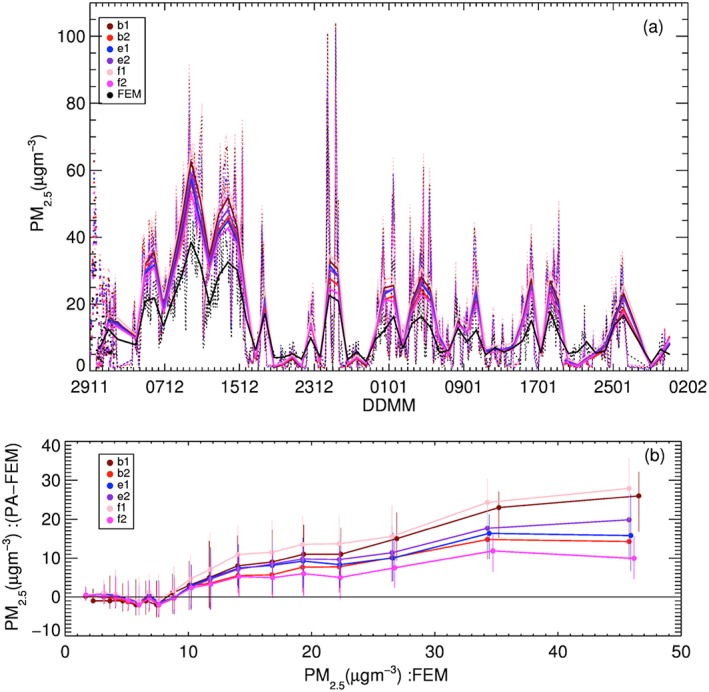
Intercomparison between PA‐II and FEM measurements of PM2.5 (a) hourly (dotted lines) and daily (solid line) mean PM2.5 from six different PA‐II nodes and FEM (black) over 8 weeks of field testing in the South Coast Air Quality Management District facility; (b) Bin‐averaged bias in PM2.5 from PA‐II nodes as a function of PM2.5 values from FEM. The three PA‐II units contained six sensors, identified as b1, b2, e1, e2, f1, and f2. PA = PurpleAir; FEM = federal equivalent method.
4. Satellite Observations
Passive satellite sensors make measurements in various regions of the electromagnetic spectrum (e.g., channels or wavelength bands), and these spectral measurements are then used to infer properties of fires and smoke. Figure 2 shows examples of fire and smoke parameters retrieved using the VIIRS aboard National Oceanic and Atmospheric Administration's Suomi‐National Polar‐orbiting Partnership satellite. There are two sets of images for each of the four variables, one taken on 8 October (before the fires started) and 9 October (after fires started) in Northern CA. In this example, the four variables include the following: true color daytime images created using the combination of red, green, and blue visible bands (RGB); night lights observed by day‐night band (VIIRS, ATBD, 2011); fire locations, as detected using thermal band anomaly techniques (Schroeder et al., 2014); and AOD at 550 nm retrieved using spectral measurements (VIIRS, ATBD, 2011). In panel (d), red indicates high AOD values (AOD > 1.0), whereas blue‐green is AOD closer to 0. While AOD is a column‐integrated value, it can help infer air quality at the surface.
Figure 2.
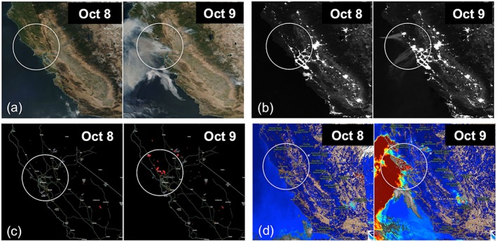
The figures show images by Visible Infrared Imaging Radiometer Suite taken on 8 October (before the fires started) and 9 October (after the fires started) in Northern CA. The observation presented here includes (a) RGB images, (b) Visible Infrared Imaging Radiometer Suite night lights, (c) thermal anomaly or fire detection, and (d) aerosol optical depth at 550 nm. The RGB, night lights, and fire images are obtained from National Aeronautics and Space Administration's worldview, whereas aerosol optical depth images were obtained from National Oceanic and Atmospheric Administration's e‐IDEA tool.
All four parameters show a clear signal of fires/smoke on 9 October, which was absent in the images taken on 8 October. The huge smoke plumes originating from multiple fires are extending from land to ocean in the RGB images; the scattering of night lights by smoke particles during the nighttime is prominently visible in day‐night band.
In addition, to retrieval on VIIRS, AOD is retrieved from NASA's MODIS aboard Aqua satellite (Aqua‐MODIS) and has a long history (Gupta et al., 2006) of being utilized to quantify the impact of fires on local and regional air quality. In the following sections, we analyze the MODIS AOD at 10‐km spatial resolution, where we have picked retrievals with the highest quality assurance and have spatially and temporally matched to point locations using the standard method (Gupta & Christopher, 2008, 2009a). In this method, a collocation represents the MODIS AOD pixel nearest to the LCAQM and the averaged LCAQM measurements taken within ±30 min from satellite overpass (approximately 13:30 local time for Aqua). The matched MODIS‐LCAQM data set is used to perform AOD‐PM2.5 analysis. The AOD data were also separately matched with EPA's AIRNOW monitors and LCAQM network in CA during October 2017.
5. Results and Discussion
5.1. LCAQMs and Satellite Responses to the Fires
Both LCAQM and satellite measurements are emerging as techniques to monitor air pollution. LCAQM can be deployed in large numbers due to their low cost to increase the spatial and temporal resolution of current air monitoring networks. Satellites are able to provide global daily observations under cloud‐free conditions. There is some similarity in the physics of these two techniques as both measure light, since the radiation is reduced (known as extinction) when it interacts (either scattered or absorbed) with the particles. Knowing that the particle/light interaction is dependent on the wavelength, both techniques must make assumptions about the particle optical properties and rely on inversion algorithms to infer the total loading (ambient concentrations or AOD) of the aerosol (King et al., 1999).
Assumption about particles properties is one of the common sources of uncertainty in both techniques. Most LCAQM provide particle counts in various size bins that are then calculated to mass concentration whereas satellite provides AOD values that can later be converted into PM2.5 mass concentrations. There are many differences between the two techniques and measurements they provide. AOD is an optical property and represents columnar loading of aerosols in the atmosphere, whereas LCAQM directly provides PM2.5 in μg/m3 measured near the surface. The satellite‐derived AOD represents large area on the earth (i.e., 100 km2 for data used in this study), whereas LCAQM is point measurements.
Despite differences between the two measurements of PM2.5, both can be related to standard FRM/FEM PM2.5 measurements and can be used to represent air quality near the surface under certain conditions. Figure 3 shows the AOD (left panels) and PM2.5 (right panels) measurements matched in space and time over LCAQM network in Northern CA on selected days in October 2017. The individual vertical bars represent the locations of LCAQM with the bar height being proportional to the magnitude of the parameter, which is also color coded. Both AOD and PM2.5 on 8 October during the MODIS‐Aqua overpass time were very low throughout the region with values of AOD < 0.2 and PM2.5 < 15.0 μg/m3. We start seeing the impact of fire and smoke in measurements made on 9 October when AOD over a specific station reached up to 1.5 with PM2.5 > 270. μg/m3. Although most of the LCAQM stations observed higher values of both AOD and PM2.5 as compared to the previous day, the impact was minimal at the stations located in the southern part of the network. This uneven distribution of smoke and its impact on PM2.5 is related to fire locations and prevailing wind conditions on that day. The 10 October case was unusual as several LCAQM monitors reported very high values, whereas satellite AODs over stations do not respond in the same manner. This behavior is partially due to the limited number of AOD retrievals from MODIS in the dense smoke plume. As discussed in this section, the satellite‐surface collocation method uses the nearest‐available AOD pixels for the comparison. Therefore, on this particular day, far away pixels with lower AOD were picked up over LCAQM stations and AOD values are low on this specific day. The air quality level over many LCAQM locations reached hazardous level (PM2.5 > 260) with MODIS AOD values as high as 2.5 on 11 October. Similar high PM concentrations and AOD values were observed on 12 and 13 October (not shown here) with lower concentrations and air quality conditions returning to normal levels on 15 October.
Figure 3.
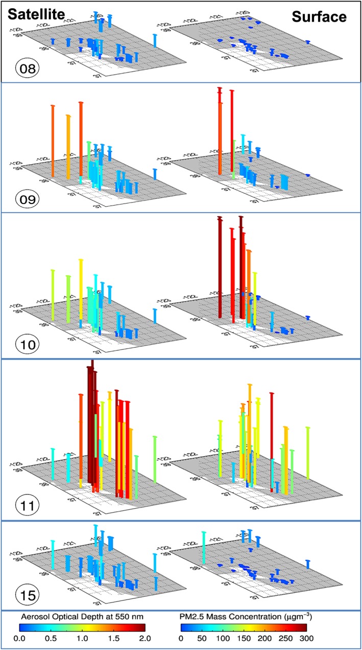
Time series of aerosol optical depth and PM2.5 in Bay Area before, during, and after, the fires. The left panels show Moderate resolution Imaging Spectroradiometer‐Aqua aerosol optical depths and the right panels show PM2.5 from low‐cost air quality monitor. The number inside the circle shows date in October 2017. The date 8 October is before fire, 9–11 October is during the fire, and 15 October is toward the end of the fires.
Figure 4 further quantifies the increase in AOD and PM2.5 at selected LCAQM locations on a weekly timescale, corresponding to the period before the fire (2–8 October), during peak fire (9–15 October), during reduced intensity of fires (16–22 October), and after fires subsided (23–29 October). The before‐fire weekly mean PM2.5 values were lower than 10 μg/m3 with AODs < 0.25. During the peak fire event, weekly PM2.5 increased up to tenfold with PM2.5 values as high as 112 μg/m3 and AODs averaged around 0.6. Note that MODIS AOD is instantaneous and represents a much larger area as compared to a point measurement taken continuously in time by LCAQM. Therefore, differences in the response to smoke loading between the two parameters are expected. The analysis presented in Figures 3 and 4 clearly show that both satellite‐derived AODs and LCAQM PM2.5 responded to the enhanced smoke loading in the region due to fires. Both data sets showed similar trends with the response being larger during the period with peak fires and near background levels before and after fires. It also suggests that AODs can be utilized in the regions with no ground monitors to assess the impact of smoke from fires on local air quality conditions (Gupta et al., 2007).
Figure 4.
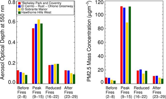
The impact of fires on local air quality conditions at weekly scale. The bar charts show weekly averaged aerosol optical depth (left) and PM2.5 (right) at selected low‐cost air quality monitor locations close to fires in Northern CA. These stations are located southeast of fires.
5.2. AOD‐PM2.5 Relationships
Through its ability to reflect and scatter solar radiation (haze), the presence of aerosols (airborne PM) can be inferred from satellite observations. Some of these space sensors offer enormous potential for monitoring air quality and climate impacts on the global scale (Gupta et al., 2006; Hoff & Christopher, 2009; van Donkelaar et al., 2010). However, these passive sensors cannot directly measure surface PM2.5 but, rather, provide an estimate of AOD, a unitless quantity that represents the perturbation of solar radiation by the particles. AOD describes the integral of aerosol loading from the surface through the top of the atmosphere, and estimating the PM concentrations near the ground (e.g., nose level) requires additional steps.
The AOD‐PM2.5 relationship can be defined by the following equation (Hoff & Christopher, 2009):
Assuming a well‐mixed boundary layer of height (H) with no overlaying aerosol layers, cloud‐free skies, and particles with similar optical properties (Hoff & Christopher, 2009), where τ is AOD, f (RH) is the ratio of ambient and dry extinction coefficients, ρ is aerosol mass density (g/m3), Q ext is Mie extinction efficiency, and r eff is the particle effective radius. We do not have good measurements of these specific aerosol properties and actual atmospheric conditions often violate the assumptions made here. Therefore, alternative techniques were developed to convert AOD to PM2.5 and they can be broadly categorized into three main groups: (a) statistical methods (Gupta & Christopher, 2009a, 2009b), (b) model scaling approach (van Donkelaar et al., 2015), and (c) satellite data assimilation into regional and global models (Buchard et al., 2015). Each technique has advantages and limitations, and their use strictly depends on applications. Hoff and Christopher (2009) provide details on each of these techniques.
Statistical models are based on the assumption that AOD can be correlated with surface PM2.5 (Figure 5; Gupta et al., 2006; Hoff & Christopher, 2009). AOD/PM2.5 correlation is greatest when most of the particles are concentrated in the lower layers of the atmosphere. In many locations of the world, AOD/PM2.5 correlations approach R = 0.75. However, the AOD‐PM2.5 relationship does not hold in situations that involve long‐range, high‐altitude transport of aerosol (e.g., wildfires and dust storms). Therefore, to establish a more precise quantitative relationship, additional information is required, which directly or indirectly controls the PM2.5 concentrations at the surface. These include planetary boundary layer height, T, RH, wind speed, and/or statistical relationships derived from selected ground monitors (Gupta & Christopher, 2009b; Hoff & Christopher, 2009; Y. Liu et al., 2005).
Figure 5.
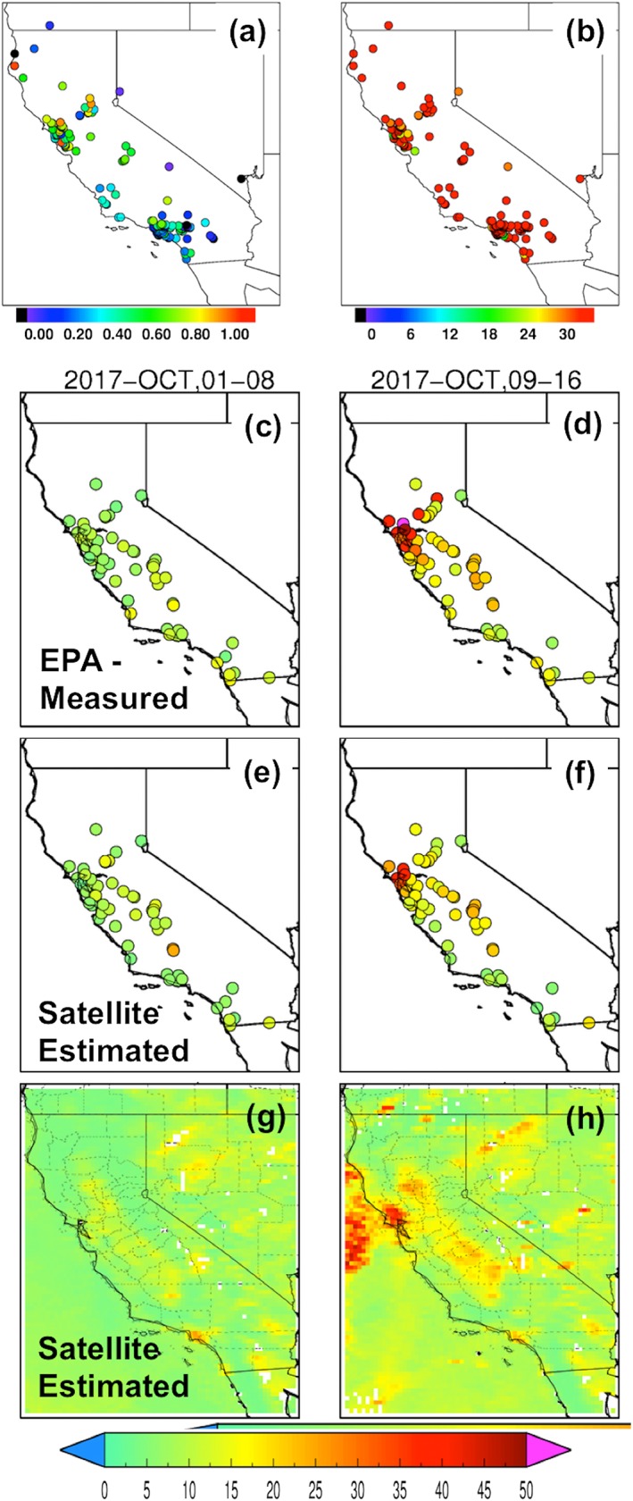
Aerosol optical depth‐PM2.5 relationship and satellite estimated PM2.5 in California over low‐cost air quality monitor (LCAQM) and EPA networks. (a) Linear correlation coefficient (R) over LCAQM; (b) Number of collocated aerosol optical depth‐PM2.5 pairs over LCAQM; (c, d) EPA measured weekly averaged PM2.5 before the fires started (1–8 October) and during the fires (9–16 October); (e,f) Satellite estimated PM2.5 over EPA network for the same period as in (c) and (d); and (g,h) Satellite estimated PM2.5 showing regional distribution before and during fires. EPA = Environmental Protection Agency.
Therefore, the statistical approach works well when meteorology and other input parameters that control PM2.5 concentration at the nose level are included. Statistical models perform well at local scale and within limited region; they also outperform two other techniques on hourly and daily scales. The main limitation, however, is that they need ground‐based monitors to build these models. Absence of ground monitors is a tremendous challenge in many parts of the world. Statistical models deliver, on many occasions, where physical processes are not well known or not controlled (van Donkelaar et al., 2015).
5.3. Correlation Analysis and PM2.5 Mapping
We determined the relationship between satellite data and LCAQM PM2.5 measurements then evaluated it using the EPA FEM data. The presence of EPA FEM data in sufficient spatial density enables evaluation of the utility of these low‐cost sensors in relating to satellite data in regions where no such FEM measurements exist or are very sparse. We have used the collocated MODIS‐LCAQM data sets (i.e., matched spatially and temporally) during October 2017 over CA to evaluate the AOD‐PM2.5 relationship. The collocated data sets consist of 3,071 pairs of AOD‐PM2.5 over 180 LCAQM locations. The linear correlation coefficient (Figure 5a) between AOD and PM2.5 is calculated for each LCAQM location with a number of AOD‐PM2.5 pairs shown in Figure 5b. The correlation varies widely over LCAQM stations, with higher values in Northern CA corresponding to high PM2.5 loading during the period. The low correlation in Southern CA could be associated with high uncertainties in MODIS AOD retrievals from the complex topography and high surface reflectance (Sayer et al., 2014). The correlation analysis is comparable to previously published research (Lee et al., 2016) in this area using standard EPA measurements. As discussed in section 5.2, the AOD‐PM2.5 relationship works very well under conditions with moderate to high aerosol loading, well‐mixed boundary layer with no secondary aerosol layers, dominated by smaller size particles and moderate RH (~40%) conditions.
In order to estimate PM2.5 using satellite observation over an entire region, we have developed a generalized geographically weighted regression model (Gupta & Christopher, 2009b) and used it to estimate PM2.5 for the month of October. The satellite‐estimated PM2.5 measurements for the week before the fires (Figure 5e and during fires Figure 5f) are compared against EPA‐measured PM2.5 (Figures 5c and 5d) over the same period. Both EPA‐measured and satellite‐estimated PM2.5 values were lower (<15 μg/m3) before the fires and enhanced multifold during the fires, with peak weekly average values up to 60 μg/m3 over the stations close to fire locations (Figure 2). Figures 5g and 5h show the spatial distribution of satellite‐estimated PM2.5 over the entire region at 0.1 × 0.1° spatial resolution before and during fires, respectively. Clearly before fires, PM2.5 values vary between low (5 μg/m3) to moderate (25 μg/m3) with homogeneous distribution across the region and over the ocean. During the fire, smoke was transported by winds in different parts of the region, and the resulting, enhanced PM2.5 values can be seen across the region. Areas within close proximity to fires show up as hot spots in this PM2.5 map. These spatial distribution maps derived from satellite are a unique advantage of satellite observations, which are very difficult to obtain from surface measurements alone. It is important to note that LCAQM data were used in the regression analysis, which are used to estimate satellite‐based PM2.5 maps. The LCAQM along with satellite observations can be very useful in places where standard measurements are not available.
6. Summary and Discussion
The role of LCAQMs and satellite observations in analyzing the impact of fires on local and regional air quality has been discussed using fires in Northern California during October 2017. We created a spatially and temporally matched satellite and surface database for the entirety of California. This database contains 3,071 matched AOD‐PM2.5 pairs covering over 180 low‐cost monitors. The LCAQM network used in this analysis uses the PA sensors (http://purpleair.com), which provides real‐time data to the public domain.
Typical performance of the PA‐II sensors was tested in the LA area under laboratory and field conditions by comparing against FEM measurements. The results showed satisfactory performance typical to previously reported studies, with observed biases up to 35% for 24‐hr average mean PM2.5 values. The sensor bias was also found to vary with increasing PM2.5 loading in the atmosphere.
The time series analysis performed using LCAQM and MODIS demonstrates that both measurements responded to change in air quality as a result of fires in Northern CA. We used LCAQM measurement along with MODIS‐derived AODs to develop geographically weighted regression models to estimate spatial maps of PM2.5 using satellite AODs. These satellite‐estimated PM2.5 values are compared against EPA's FEM values and are found to have good agreement. The results demonstrate the utility of such low‐cost sensors to relate AOD data to surface PM2.5 in the absence of traditional FEM instruments. Our case study leveraged the high spatial density of FEM in our study area to perform these comparisons. Our findings here suggest that the use of low‐cost air quality sensors may be a viable option to improve the AOD‐PM2.5 relationship for locations with no or limited surface monitoring. To our knowledge, this is the first study that demonstrates the application of such low‐cost monitors for relating AOD to surface PM2.5 data.
Our current study demonstrated the application of such low‐cost sensors for high aerosol loading conditions when the satellite retrievals may be subject to smaller uncertainties compared to background or clean conditions. Further, the sensor data were used without any corrections, which did not appear to impact the performance of AOD‐PM2.5 models, likely due to the high concentrations measured. These limitations are future research questions to be addressed. Nevertheless, the successful application of such sensors to augment and/or improve satellite data for a specific case study, without the integration of traditional surface measurements, is a useful finding. The study has significant implications: (1) Low‐cost air quality sensors may be a useful alternative to traditional FEM monitors for the purpose of improving the satellite‐derived PM2.5 estimates and (2) The increase in the spatial resolution of surface PM2.5 data derived from both satellites and LCAQM has tremendous applications in evaluating personal exposures and assessing health impacts.
While the current network of FRM and FEM PM monitors across the United States provides quality measurements for determining regional attainment and regulatory decision making, a dense network of LCAQMs can provide measurements for exceptional events, such as the fires in Northern California.
The following quote from Hoff and Christopher (2009) correctly highlights the strength, limitation, and the way forward on the use of satellite observations in air quality monitoring. “Satellite measurements are going to be an integral part of the Global Earth Observing System of Systems. Satellite measurements by themselves have a role in air quality studies but cannot stand alone as an observing system. Data assimilation of satellite and ground‐based measurements into forecast models has synergy that aids all of these air quality tools.”
Acknowledgments
This work was supported by the NASA ROSES program NNH16ZDA001N‐CSESP: Citizen Science for Earth Systems Program managed by Kevin Murphy under cooperative agreement NNX17AG68A. The findings presented here have not been reviewed by the funding agency and our affiliated organizations and do not represent official policy. We thank the MODIS science team for their efforts to maintain and improve the radiometric quality of MODIS data and LAADS/MODAPS for the continued processing of the MODIS products. The authors are thankful to the PurpleAir team for the creation and continued stewardship of the open‐source low‐cost air quality data record, which is available from http://www.purpleair.com. Use of sensor manufacturer name does not imply endorsement.
Gupta, P. , Doraiswamy, P. , Levy, R. , Pikelnaya, O. , Maibach, J. , Feenstra, B. , et al. (2018). Impact of California fires on local and regional air quality: The role of a low‐cost sensor network and satellite observations. GeoHealth, 2, 172–181. 10.1029/2018GH000136
References
- Black, C. , Tesfaigzi, Y. , Bassein, J. A. , & Miller, L. A. (2017). Wildfire smoke exposure and human health: Significant gaps in research for a growing public health issue. Environmental Toxicology and Pharmacology, 55, 186–195. 10.1016/j.etap.2017.08.022 [DOI] [PMC free article] [PubMed] [Google Scholar]
- Buchard, V. , da Silva, A. M. , Colarco, P. R. , Darmenov, A. , Randles, C. A. , Govindaraju, R. , et al. (2015). Using the OMI aerosol index and absorption aerosol optical depth to evaluate the NASA MERRA aerosol reanalysis. Atmospheric Chemistry and Physics, 15(10), 5743–5760. 10.5194/acp-15-5743-2015 [DOI] [Google Scholar]
- CALFIRE (2017, October 30, 2017). California statewide fire summary. Retrieved from http://calfire.ca.gov/communications/communications_StatewideFireSummary
- Cascio, W. E. (2018). Wildland fire smoke and human health. Science of the Total Environment, 624, 586–595. 10.1016/j.scitotenv.2017.12.086 [DOI] [PMC free article] [PubMed] [Google Scholar]
- Fann, N. , Alman, B. , Broome, R. A. , Morgan, G. G. , Johnston, F. H. , Pouliot, G. , & Rappold, A. G. (2018). The health impacts and economic value of wildland fire episodes in the U.S.: 2008–2012. Science of the Total Environment, 610‐611, 802–809. 10.1016/j.scitotenv.2017.08.024 [DOI] [PMC free article] [PubMed] [Google Scholar]
- Giglio, L. , Schroeder, W. , & Justice, C. O. (2016). The collection 6 MODIS active fire detection algorithm and fire products. Remote Sensing of Environment, 178, 31–41. 10.1016/j.rse.2016.02.054 [DOI] [PMC free article] [PubMed] [Google Scholar]
- Gupta, P. , & Christopher, S. A. (2008). Seven year particulate matter air quality assessment from surface and satellite measurements. Atmospheric Chemistry and Physics, 8(12), 3311–3324. 10.5194/acp-8-3311-2008 [DOI] [Google Scholar]
- Gupta, P. , & Christopher, S. A. (2009a). Particulate matter air quality assessment using integrated surface, satellite, and meteorological products: 2. A neural network approach. Journal of Geophysical Research, 114, D20205 10.1029/2008JD011497 [DOI] [Google Scholar]
- Gupta, P. , & Christopher, S. A. (2009b). Particulate matter air quality assessment using integrated surface, satellite, and meteorological products: Multiple regression approach. Journal of Geophysical Research, 114, D14205 10.1029/2008JD011496 [DOI] [Google Scholar]
- Gupta, P. , Christopher, S. A. , Box, M. A. , & Box, G. A. (2007). Multi year satellite remote sensing of particulate matter air quality over Sydney, Australia. International Journal of Remote Sensing, 28(20). 10.1080/01431160701241738 [DOI] [Google Scholar]
- Gupta, P. , Christopher, S. A. , Wang, J. , Gehrig, R. , Lee, Y. , & Kumar, N. (2006). Satellite remote sensing of particulate matter and air quality assessment over global cities. Atmospheric Environment, 40(30), 5880–5892. 10.1016/j.atmosenv.2006.03.016 [DOI] [Google Scholar]
- Ho, V. , & Lyons, J. (2017, October 15, 2017). Live updates: Northern Calif. wildfires cause estimated $3 billion damage; death toll still 40. San Francisco Chronical.
- Hoff, R. M. , & Christopher, S. A. (2009). Remote sensing of particulate pollution from space: Have we reached the promised land? Journal of the Air & Waste Management Association, 59(6), 645–675. 10.3155/1047-3289.59.6.645 [DOI] [PubMed] [Google Scholar]
- Jayaratne, R. , Liu, X. , Thai, P. , Dunbabin, M. , & Morawska, L. (2018). The influence of humidity on the performance of low‐cost air particle mass sensors and the effect of atmospheric fog. Atmospheric Measurement Techniques Discussions. 10.5194/amt-2018-100 [DOI] [Google Scholar]
- Jiao, W. , Hagler, G. , Williams, R. , Sharpe, R. , Brown, R. , Garver, D. , et al. (2016). Community Air Sensor Network (CAIRSENSE) project: Evaluation of low‐cost sensor performance in a suburban environment in the southeastern United States. Atmospheric Measurement Techniques, 9(11), 5281–5292. 10.5194/amt-9-5281-2016 [DOI] [PMC free article] [PubMed] [Google Scholar]
- Kasler, D. (2017, December 6, 2017). Wine country wildfire costs now top $9 billion, costliest in California history. The Sacramento Bee.
- King, M. D. , Kaufman, Y. J. , Tanr‚, D. , & Nakajima, T. (1999). Remote sensing of tropospheric aerosols from space: Past, present, and future. Bulletin of the American Meteorological Society, 80(11), 2229–2259. [Google Scholar]
- Lee, H. J. , Chatfield, R. B. , & Strawa, A. W. (2016). Enhancing the applicability of satellite remote sensing for PM2.5 estimation using MODIS Deep Blue AOD and land use regression in California, United States. Environmental Science & Technology, 50(12), 6546–6555. 10.1021/acs.est.6b01438 [DOI] [PubMed] [Google Scholar]
- Levy, R. C. , Mattoo, S. , Munchak, L. A. , Remer, L. A. , Sayer, A. M. , Patadia, F. , & Hsu, N. C. (2013). The Collection 6 MODIS aerosol products over land and ocean. Atmospheric Measurement Techniques, 6(11), 2989–3034. 10.5194/amt-6-2989-2013 [DOI] [Google Scholar]
- Liu, Y. , Sarnat, J. A. , Kilaru, A. , Jacob, D. J. , & Koutrakis, P. (2005). Estimating ground‐level PM2.5 in the eastern United States using satellite remote sensing. Environmental Science & Technology, 39(9), 3269–3278. [DOI] [PubMed] [Google Scholar]
- Liu, Z. , Winker, D. , Omar, A. , Vaughan, M. , Kar, J. , Trepte, C. , et al. (2015). Evaluation of CALIOP 532 nm aerosol optical depth over opaque water clouds. Atmospheric Chemistry and Physics, 15(3), 1265–1288. 10.5194/acp-15-1265-2015 [DOI] [Google Scholar]
- Pimlott, K. , Laird, J. , & Brown Jr, E. G. (2016). 2016 wildfire activity statistics.
- Sayer, A. M. , Munchak, L. A. , Hsu, N. C. , Levy, R. C. , Bettenhausen, C. , & Jeong, M. J. (2014). MODIS Collection 6 aerosol products: Comparison between Aqua's e‐Deep Blue, Dark Target, and “merged” data sets, and usage recommendations. Journal of Geophysical Research: Atmospheres, 119, 13,965–13,989. 10.1002/2014JD022453 [DOI] [Google Scholar]
- Schroeder, W. , Oliva, P. , Giglio, L. , & Csiszar, I. A. (2014). The new VIIRS 375 m active fire detection data product: Algorithm description and initial assessment. Remote Sensing of Environment, 143, 85–96. 10.1016/j.rse.2013.12.008 [DOI] [Google Scholar]
- Sigsgaard, T. , Forsberg, B. , Annesi‐Maesano, I. , Blomberg, A. , Bølling, A. , Boman, C. , et al. (2015). Health impacts of anthropogenic biomass burning in the developed world. European Respiratory Journal, 46(6), 1577–1588. 10.1183/13993003.01865-2014 [DOI] [PubMed] [Google Scholar]
- Snik, F. , Rietjens, J. H. H. , Apituley, A. , Volten, H. , Mijling, B. , Di Noia, A. , et al. (2014). Mapping atmospheric aerosols with a citizen science network of smartphone spectropolarimeters. Geophysical Research Letters, 41, 7351–7358. 10.1002/2014GL061462 [DOI] [Google Scholar]
- van Donkelaar, A. , Martin, R. V. , Brauer, M. , & Boys, B. L. (2015). Use of satellite observations for long‐term exposure assessment of global concentrations of fine particulate matter. Environmental Health Perspectives, 123(2), 135–143. 10.1289/ehp.1408646 [DOI] [PMC free article] [PubMed] [Google Scholar]
- van Donkelaar, A. , Martin, R. V. , Brauer, M. , Kahn, R. , Levy, R. , Verduzco, C. , & Villeneuve, P. J. (2010). Global estimates of ambient fine particulate matter concentrations from satellite‐based aerosol optical depth: Development and application. Environmental Health Perspectives, 118(6), 847–855. 10.1289/ehp.0901623 [DOI] [PMC free article] [PubMed] [Google Scholar]
- VIIRS , & ATBD (2011). Joint Polar Satellite System (JPSS) VIIRS imagery products Algorithm Theoretical Basis Document (ATBD).
- Youssouf, H. , Liousse, C. , Roblou, L. , Assamoi, E.‐M. , Salonen, R. , Maesano, C. , et al. (2014). Non‐accidental health impacts of wildfire smoke. International Journal of Environmental Research and Public Health, 11(11), 11772. [DOI] [PMC free article] [PubMed] [Google Scholar]