Estimation of in vivo constitutive parameters of the aortic wall using a machine learning approach

Abstract

The patient-specific biomechanical analysis of the aorta requires the quantification of the in vivo mechanical properties of individual patients. Current inverse approaches have attempted to estimate the nonlinear, anisotropic material parameters from in vivo image data using certain optimization schemes. However, since such inverse methods are dependent on iterative nonlinear optimization, these methods are highly computation-intensive. A potential paradigm-changing solution to the bottleneck associated with patient-specific computational modeling is to incorporate machine learning (ML) algorithms to expedite the procedure of in vivo material parameter identification. In this paper, we developed an ML-based approach to estimate the material parameters from three-dimensional aorta geometries obtained at two different blood pressure (i.e., systolic and diastolic) levels. The nonlinear relationship between the two loaded shapes and the constitutive parameters are established by an ML-model, which was trained and tested using finite element (FE) simulation datasets. Cross-validations were used to adjust the ML-model structure on a training/validation dataset. The accuracy of the ML-model was examined using a testing dataset.

1. INTRODUCTION

With advances in medical imaging modalities and computation power, numerical simulations of the cardiovascular structure such as the aorta, which utilizes the patient-specific three-dimensional (3D) geometry, have been increasingly pursued in the past decade [1], Yet, the difficulty in obtaining in vivo patient-specific elastic properties of the aortic wall from clinical cardiac images has been one of the biggest obstacles in patient-specific biomechanical analysis. This has motivated recent efforts to develop inverse methods for estimating the in vivo material properties of the aortic wall on a patient-specific basis. In these methods, deformations and boundary conditions are used to inversely estimate the material parameters of a particular constitutive model. However, the complex 3D shapes and nonlinear and anisotropic constitutive behavior make this task challenging.

To reduce computational complexity, some studies suggested the use of simplifications in material models and/or geometries. For example, Liu and Shi [2], Zhang and co-workers [3] and Franquet and co-workers [4] identified linear elastic material parameters. By assuming a perfect cylindrical shape of the arteries, Schulze-Bauer and Holzapfel [5] identified Fung-type material parameters, Stalhand, Olsson and Klarbring, Masson and co-workers [6–9] estimated material parameters using the constitutive model proposed by Holzapfel and co-workers [10], and Smoljkic and co-workers [11] estimated the Gasser-Ogden-Holzapfel (GOH) model [12] parameters. Liu and co-workers [13] also determined the modified Moony-Rivlin parameters of the carotid artery reconstructed from magnetic resonance imaging (MRI).

To fully exploit the 3D geometries reconstructed from medical image data, the current methods for in vivo material parameter estimation largely rely on various optimization schemes. In these optimization-based inverse methods, an objective/error function is built upon the difference between predicted and image-derived physical fields (e.g. coordinates of diastolic geometry and diastolic-to-systolic strain field), and then the constitutive parameters are iteratively adjusted until the objective function is minimized. Specifically, Starting from an initial guess of the constitutive parameters, the inverse methods usually involve the following steps: (1) recovering an unloaded state from a known loaded state (e.g. systole); (2) predicting the desired physical field of another loaded state (e.g. diastole) through computational analysis, which is referred by numerically-predicted physical field; and (3) the constitutive parameters are iteratively fine-tuned by a nonlinear optimization algorithm until the numerically-predicted physical field matches with the image-derived physical field at the loaded state (e.g. diastole). This optimization process yields the optimal constitutive parameters. Using finite element (FE) updating schemes, Wittek and co-workers [14, 15] developed two methods to determine GOH material parameters of the human abdominal aorta from in vivo 4D ultrasound data [16], However, numerous iterations were needed to reach the optimal solution with a long computing time of 1–2 weeks. Such high computational cost could inhibit a practical use of these methods, particularly in a clinical setting requiring rapid feedback to clinicians. To this end, our group has recently proposed two optimization-based methods to expedite the estimation process. The multi-resolution direct search (MRDS) approach [17] was designed to improve the searching algorithm, and the computation time was reduced to 1–2 days with similar CPU and memory. Due to static determinacy, given loading and boundary conditions as well as geometry, stress can also be directly computed from clinical images [18–20], Therefore, we developed a stress-based inverse approach [21], in which the computationally-expensive FE simulations were avoided by building the objective function upon stresses, and the optimization was completed in approximately 2 hours. However, optimization-based inverse methods are inherently limited by their iterative nature, and any further improvement of computational speed can be difficult.

Recently, machine learning (ML) techniques, particularly deep learning (DL) [22–24], have garnered enormous attention in the field of artificial intelligence, leading to revolutionary breakthroughs in many applications [22, 25–31], ML approaches have been developed for biomechanical analysis. For instance, Luo and co-workers [32] developed ML classifiers to infer strength of ascending thoracic aneurysm from elastic properties, Cilia and co-workers proposed ML techniques for obtaining the GOH model parameters from uniaxial data [33], ML-models are capable of establishing complex and nonlinear relationship between inputs and outputs. A potential paradigm-changing solution to the bottlenecks associated with patient-specific computational modeling is to incorporate ML algorithms to expedite the procedure of in vivo material parameter identification. By designing and training an ML-model on a large dataset, it may automatically produce the required outputs (constitutive parameters) directly from necessary inputs (multi-phase aorta shapes), without the need for costly iterative schemes. Thus, once trained, the ML-model can instantaneously predict the material parameters.

In this paper, we developed an ML-based approach to identify the material parameters of the GOH constitutive model. As depicted in Figure 1, the inputs to this ML-model are the aorta geometries at two distinct blood pressure levels, namely the systolic and diastolic geometries, which were also used by our previous optimization-based inverse approaches [17, 21], An ML-model was built to establish the nonlinear relationship between the geometries and the constitutive parameters. The proposed ML-model consists of an unsupervised shape encoding module using principal component analysis and a supervised nonlinear mapping module using a neural network. The datasets for training, validation and testing were generated from FE simulations. Please note that the numerically-generated data may not represent the real patient geometries. Cross-validations were used to adjust the neural network structure. The accuracy of the ML-model prediction was examined using a testing dataset.

Figure 1.

The proposed machine learning (ML) approach.

2. METHODS

2.1. Constitutive model

A strain invariant-based fiber reinforced hyperelastic formulation based on the work of Gasser and co-workers [12] was used to model the constitutive relations of the aortic wall. The deformation gradient F can be multiplicatively decomposed into

$$F=\left({\text{J}}^{1/3}I\right)\overline{F},$$ (1)

where J is the determinant of F, and I is the identity tensor. $\overline{\text{F}}$ represents the volume-preserving (isochoric) part of the deformation gradient, while (J¹/³I) represents the volumetric part. The right Cauchy-Green tensor C and its isochoric counterpart $\overline{\text{C}}$ is defined as

$$C=F^{T}F,\overline{C}={\overline{F}}^T\overline{F}.$$ (2)

The isochoric strain invariants ${\overline{I}}_1\text{and}{\overline{I}}_{4i}(i=1,2)$ are defined using

$${\overline{I}}_1=tr(\overline{C}),{\overline{\mathrm{I}}}_{4i}=a_{0i}\cdot \left(\overline{C}{a}_{0i}\right),$$ (3)

where vectors a₀₁ = (cos θ, sin θ, 0) and a₀₂ = (cos θ, — sin θ, 0) characterize the two mean fiber directions in the reference configuration. θ is the angle between a mean fiber direction and the circumferential direction. Thus, ${\overline{I}}_{4i}(i=1,2)$ are equal to squares of the stretches in mean fiber directions. The total strain energy function ψ can be additively split into isochoric isotropic ${\overline{\Psi }}_{iso}$, isochoric anisotropic ${\overline{\Psi }}_{\mathit{\text{aniso}}}$ and volumetric ${\Psi }_{vol}$ parts, according to

$$\Psi \left(C,a_{0i}\right)={\overline{\Psi }}_{iso}(\overline{C})+{\overline{\Psi }}_{\text{aniso}}\left(\overline{C},a_{0i}\right)+{\Psi }_{vol}(\text{J}).$$ (4)

The isotropic matrix material is characterized by the Neo-Hookean strain energy

$${\overline{\Psi }}_{iso}(\overline{C})=C_{10}\left({\overline{I}}_1-3\right),$$ (5)

where C₁₀ is a material parameter to describe the matrix material. The isochoric anisotropic term is given by

$${\overline{\Psi }}_{\text{aniso}}\left(\overline{C},a_{0i}\right)=\frac{k_1}{2k_2}\sum _{i=1}^2\left[\exp \left\{k_2{\left[\kappa {\overline{I}}_1+(1-3\kappa ){\overline{I}}_{4i}-1\right]}^2\right\}-1\right]$$ (6)

Where k₁ is a positive material parameter that has the same unit of stress, while k₂ is a unitless material parameter, $\kappa \in (0,1/3)$ describes the dispersion of fibers. Finally, we assume that the material is nearly incompressible (slightly compressible), the volumetric term is defined by

$${\Psi }_{vol}(\text{J})=\frac{1}{D}\left[\frac{J^2-1}{2}-\ln J\right]$$ (7)

Where D is a constant that enforces material incompressibility and it is fixed to 5 × 10⁻⁴. Thus, the aortic wall tissue is characterized by five constitute parameters $\left\{C_{10},k_1,k_2,\kappa ,\theta \right\}.$ The task for the ML-model is to identify the five constitute parameters given the two-phase aorta shapes.

2.2. Generating the training/validation dataset and the testing dataset

The proposed ML model will establish a mapping between the inputs (geometries) to the outputs (material parameters) based on example input-output pairs. Each input-output pair consists of two geometries and the corresponding material parameters. To fine-tune the ML-model for optimal performance, cross-validation is used in the training phase, where the input-output pairs are partitioned into two subsets, called training set and validation set. The ML-model is trained on the training set, and its performance is assessed using the validation set. After the training phase, the accuracy of the ML-model prediction is evaluated on a new set of input-output pairs, i.e., the testing set.

In this study, the datasets are gathered from FE simulations. Using statistical modeling methods, a large number of material parameter sets are generated from 65 sets of experimentally-derived material parameters, and virtual aorta geometries at one physiological phase (i.e., systole) are generated from 3D CT images of 25 real patients. The diastolic aorta geometries are determined from FE simulations using the virtual systolic geometries and the generated material parameters. Finally, the training/validation dataset and the testing dataset consist of 15366 and 225 input-output pairs, respectively. The detailed procedures to generate the datasets are presented in the following subsections.

2.2.1. Sampling the material parameter space

In previous studies [34, 35], we have collected resected ascending thoracic aortic aneurysm (ATAA) tissue samples a total of 65 patients who underwent elective surgeries at Yale-New Haven Hospital, CT, USA between the years of 2008 and 2010, following an IRB-approved protocol. Seven-protocol biaxial tension experiments were carried out on the 65 aneurysmal patients, and five material parameters of the GOH model were determined by fitting the experimentally-obtained stress-strain curves. The material properties of patient i was represented by a vector in $y^{(i)}(i=1,2,\dots ,65),$ with its five components corresponding to five GOH parameters, and the set Y contained only the 65 vectors. These vectors are visualized in the material parameter space in Figure 2, which shows that these experimentally-derived parameters are highly clustered in certain regions. To uniformly sample the material parameter space, a convex hull of the experimentally-derived parameters was built. The convex hull is essentially a set comprised of convex combinations of all vectors of Y,

$$Conv(Y)=\left\{y=\sum _{i=1}^{65}{a}_i{y}^{(i)}|y^{(i)}\in Y,i=1,2,\dots ,65,a_i\ge 0\forall i,\sum _{i=1}^{65}{a}_i=1\right\}$$ (8)

where y isa vector in the convex hull, and a_i (i = 1, 2,…, 65) are non-negative coefficients that sum up to 1. Next, samples were draw from a uniform distribution inside the convex hull using the Gibbs sampler [36], 125 and 15 samples were generated for the training/ validation set and the testing set, respectively, as shown in Figure 2.

Figure 2.

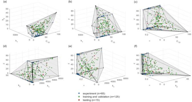
Datasets projected in 3D material parameter subspaces. The convex hull is plotted in the 3D subspaces for illustrative purpose.

2.2.2. Obtaining the virtual aorta geometries at the systolic phase

From a previous study [37], out of the 65 patients whose samples were collected for biaxial tests, deidentified clinical cardiac CT scans of 25 patients were obtained from Yale-New Haven Hospital. A set of approximately 100–150 axial CT images with a resolution of 0.7 mm x 0.7 mm x 2.5 mm containing the thoracic aorta were obtained for each patient. All patients underwent cardiac CT scans because of suspected ATAA prior to elective repair. A statistical shape model (SSM) was built from the 25 real aorta shapes at the systolic phase in a previous study [38], The SSM model describes the probability distribution of aorta shapes among the patient population using 3 modes of variations. As a result, a systolic geometry can be represented by a set of SSM parameters {C₁, C₂, C₃} described in detail in [38], The SSM parameters were standardized by their standard deviations, for example, {C_1; C₂, C₃} = {0,0,0} represents the mean shape and {C₁, C₂, C₃} = {2,0,0} represents a shape that is 2 standard deviations away from the mean shape along the first mode of variation.

For the training and validation datasets, a total number of 125 virtual aorta shapes at systolic phase were obtained by sampling the SSM parameter space {C₁, C₂, C₃} with equally spaced points in the range of −2 to 2 , i.e., within 2 standard deviations of the mean shape, as shown in Figure 3. Similarly, for the testing dataset, the SSM parameter space was sampled within 1.5 standard deviations of the mean shape. Hence, 15 systolic shapes were obtained for the testing dataset. The resulting samples in the SSM parameter space are plotted in Figure 3.

Figure 3.

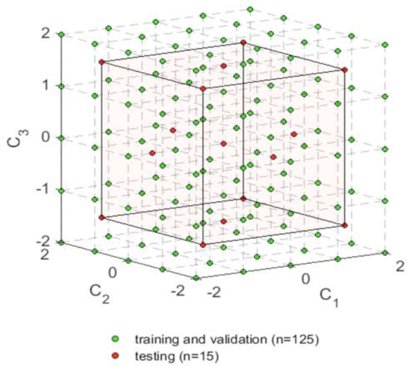
Sampling the SSM parameter spaces.

These sampled shapes are, in general, significantly differ from each other. Some representative systolic aorta shapes are plotted in Figure 4. The shapes are color-coded with curvature values obtained from Paraview 5.0.0.

Figure 4.

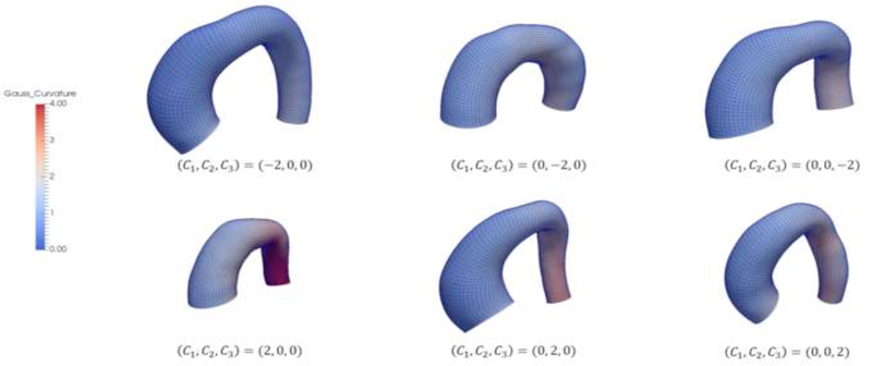
Systolic aorta shapes corresponding to some representative sets of SSM parameters. The shapes are color-coded with curvature values.

2.2.3. Generating the virtual aorta geometries at the diastolic phase using FE simulations

The virtual aorta geometries obtained from the SSM parameter space were at the systolic phase, which should be in equilibrium with the systolic physiological load. Therefore, the generalized pre-stressing algorithm (GPA) [39] was utilized to incorporate the pre-stress induced by the systolic pressure (16 kPa). In the GPA algorithm, the total deformation gradient F_t is stored as a history variable for each integration point. The F_t is updated based on the incremental deformation gradient ΔF resulting from the prescribed loading and boundary conditions.

$$F_{t+1}=\Delta F{F}_t.$$ (9)

The incremental deformation gradient ΔF resulting from the systolic pressure is iteratively applied to the virtual systolic geometries and stored in F_t. However, as illustrated in [39] , the resulted equilibrium configuration may slightly deviate from the original configuration, depending on the step size. The systolic geometries at the equilibrium configurations were used by the ML-model in the subsequent sections. Next, using a set of material parameters, the virtual aorta geometries at the diastolic phase were determined by depressurizing the systolic geometries to the diastolic phase (10 kPa).

For the training and validation sets, given one of the 125 shapes at the systolic phase and one of the 125 sets of material parameters, the virtual aorta geometry at the diastolic phase was determined through FE simulation. As shown in Figure 5, if a FE simulation converges, the input-output pair (systolic and diastolic geometries and a set of material parameters) is collected for training/validation. A total of 15,625 cases (125 materials × 125 shapes) were simulated, out of them, 259 cases were not able to converge. The convergence issues might be due to extreme shapes and/or material properties. As a result, 15366 sets of geometries with known material parameters were obtained. Similarly, for the testing set, 225 input-output pairs were generated from 15 systolic geometries and 15 sets of material parameters (all converged).

Figure 5.

The procedure to generate aorta geometries at systole and diastole. The number in the parenthesis indicates the testing dataset.

The GPA algorithm was implemented in ABAQUS user subroutine UMAT. In the FE simulations, C3D8H solid elements were used, a uniform wall thickness at the systolic phase (1.5 mm) was assumed based on the average value from [38], and pressure was applied uniformly to the inner surface of the aorta models. For the FE models, the longitudinal direction (zz) was defined using the center line of the aorta geometry. Then, the outward normal direction (rr) of each element in the inner surface of the aortic wall was obtained. The circumferential direction (θθ) was defined by taking cross product of the longitudinal and outward normal directions. The boundary nodes of the aorta models, i.e. the proximal and distal ends of the model, were only allowed to move in the radial direction defined by the local coordinate system.

2.3. The machine learning model

The machine learning model consists of an unsupervised shape encoding module and a nonlinear mapping module. The systolic and diastolic shapes are encoded by shape codes. The nonlinear mapping between the shape codes and the material parameters is established by a neural network.

2.3.1. Shape encoding

3D geometries are usually represented by FE meshes with a large number of nodes and elements. A shape corresponds to a long vector X of nodal coordinates. However, directly linking the shape X to the material parameters by a neural network, although possible, can lead to a large number of undetermined parameters that require a very large training dataset. A compact representation (i.e. shape code) of a shape can be obtained in a shape encoding procedure. The principal component analysis (PCA) [40] is widely adopted as a shape encoding method and an unsupervised learning technique for dimensionality reduction, in which the original data can be well approximated by a linear combination of a few principal components. PCA starts from assembling the covariance matrix C, given by

$$C=\frac{1}{K}\sum _{k=1}^K\left(X^{(k)}-\overline{X}\right){\left(X^{(k)}-\overline{X}\right)}^{\prime }$$ (10)

where superscript k represents patient index and K is the total number of patients. In our case, K = 25. $\overline{X}=\frac{1}{K}\sum _{k=1}^K{X}^{(k)}$ is the mean shape. Then, the eigenvalues and eigenvectors of the covariance matrix can be calculated via singular value decomposition. Thus, a shape X can be represented by

$$X\approx \overline{X}+\sum _{i=1}^m{c}_i\sqrt{{\mu }_i}{V}_i$$ (11)

where V_i and μ_i are the eigenvectors (i.e. modes of shape variations) and eigenvalues of the covariance matrix, respectively, m is the number of modes used for approximation. The shape code $\left\{c_i,i=1,\dots ,m\right\}$ can be obtained by

$$c_i={\mathit{V}}_i^T(X-\overline{X})/\sqrt{{\mu }_i}$$ (12)

where $V_i^T$ is the transpose of the column vector V_i. The first 12 modes (m=12) were retained for both the systolic and diastolic shape encoding, with the average PCA approximation error being less than 0.1%. Note that as mentioned in Section 2.2.3, the systolic geometries from GPA were slightly different from the original configuration from the SSM, and therefore 3 modes, as used in our previous study [38], are not enough to capture the shape variations for systolic geometries. We denote the systolic shape code as α_i, diastolic shape code as β_i, i = 1, 2,…, 12.

2.3.2. Nonlinear mapping

The nonlinear mapping module will map the shape codes of the two input shapes to the five material parameters, which is equivalent to establishing five nonlinear functions

$$y_k=g_k\left({\alpha }_1,\dots ,{\alpha }_{12},{\beta }_1,\dots ,{\beta }_{12}\right),k=1,2,\dots ,5$$ (13)

The inputs are the shape codes α_i and β_i, i = 1,2,…, 12, for diastolic and systolic geometries, respectively. The outputs are y_k (k = 1,2,…, 5), correspond to the five material parameters $\left\{C_{10},k_1,k_2,\kappa ,\theta \right\}.$

Neural network is, in general, flexible and can be used as universal function approximation. As shown in Figure 6, a neural network is constructed as the nonlinear mapping module. It consists of feedforward fully-connected units (neurons). Each unit has multiple inputs and a single output. For the jth unit of the i^th layer, a linear combination of the input vector zⁱ, with weight vector $W_j^i$ and offset $b_j^i,$ is computed as

$$u_j^i=w_j^{i^T}{z}^i+b_j^i$$ (14)

where the superscript i denote the index of layer, and subscript j denote the index of unit in the layer. zⁱ is a column vector of ${\left[Z_1^i,Z_2^i,\dots ,Z_{n_i}^i\right]}^T,$ and n_i is the number of units in the i^th layer. The weighted sum $u_j^i$ is nonlinearly transformed into the output $Z_j^{i+1}$ using an activation function.

$$z_j^{i+1}=f\left(u_j^i\right)$$ (15)

The softplus [41] activation function was used, which is given by

$$f(u)=\log (1+\mathit{\text{exp}}(u))$$ (16)

This function is a smooth version of the rectified linear unit (ReLU) [42, 43], As demonstrated in the discussion section, other activation functions can lead to large testing errors in our application. The neural network has two hidden layers with the same number of softplus units, and the output layer has 5 softplus units.

Figure 6.

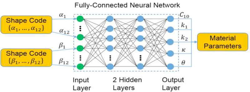
The neural network for mapping the shape codes to the material parameters. The green dots represents the input layer, and the blue dots represent the softplus units in the hidden layers and the output layer of the neural network.

The neural network was implemented using Tensorflow [44], The inputs and outputs were normalized using the maximum absolute value of each dimension. Consequently, the normalized shape codes are within the range of −1 to 1, and the normalized material parameters are within the range of 0 to 1. The mean squared error (MSE) was used as the loss function

$$MSE=\sum _{k=1}^5\frac{1}{N}\sum _{l=1}^N({\overline{y}}_k^l-{\hat{\overline{y}}}_{\kappa }^{(l)}{)}^2$$ (17)

where l is the index for an input-output pair, N is the total number of input-output pairs, ${\hat{\overline{y}}}_k^l$ and ${\stackrel{⌢}{\overline{y}}}_k^{(l)}$ represent the k^th actual and predicted normalized material parameters, respectively. After the nonlinear mapping, the predicted material parameters were rescaled to its original range. The parameters of the neural network were obtained through the Adamax optimization algorithm [45] , For detailed theories, please refer to [46], The network structure, i.e., number of hidden layers and number of units was determined through cross-validations in Section 2.4.

2.4. Training, adjusting and testing the ML-model

The unsupervised shape encoding module was trained only using the training and validation sets, i.e., the mean shape $\overline{X},$ eigenvectors V_i and eigenvalues μ_i of the covariance were computed only using the training and validation data. Since shapes in the testing set are different from those in the training and validation sets, the testing shape codes were obtained from Eqn.(12) using $\overline{X},$ V_i and μ_i computed from the training and validation sets.

Using the training/validation dataset, the performance of the nonlinear mapping module was assessed through leave-one-out (LOO) cross-validation, and the neural network structure was fine-tuned. As depicted in Figure 7, in each round of the LOO cross-validation, the data was split into a training set and a validation set, according to the material parameters. We pick one set of material parameters (and its corresponding geometries) from the 125 sets from Section 2.2.1 as the validation set, and train the neural network on the remaining 124 sets (and its corresponding geometries). An averaged error was obtained after repeating this procedure for all of the 125 sets of material parameters. Hence, the training set never contains the material information used in the validation. Similarly, ten-fold cross-validation can be performed by splitting according to sets of material parameters.

Figure 7.

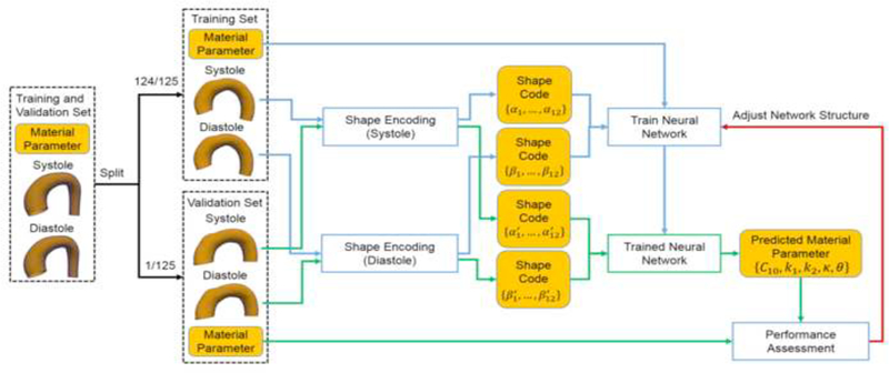
Adjusting the network structure using the leave-one-out (LOO) cross-validation.

The discrepancy between the actual and predicted material parameters was quantified by normalized mean absolute error (NMAE). The absolute error (AE) for the k^th material parameter is defined by

$$A{E}_k^{(l)}=\left|y_k^{(l)}-{\widehat{y}}_k^{(l)}\right|$$ (18)

where index l and k are the same as Eqn.(17), $y_k^{(l)}\text{and}{\widehat{y}}_k^{(l)}$ represent the k^th actual and predicted material parameter, respectively. The NMAE of the k^th material parameter is defined by

$$NMA{E}_k=\frac{{\sum }_{l=1}^{N}A{E}_k^{(l)}}{N\left({\max }_l\left(y_k^{(l)}\right)-{\min }_l\left(y_k^{(l)}\right)\right)}\times 100\%$$ (19)

where N is defined in (Eqn.17). Next, the number of units in each layer was adjusted in the range of 32 to 512 to minimize the averaged NMAE in the LOO and ten-fold cross-validations. Resulting performance for different network structures is summarized in Table 1 and Table 2. We evaluated neural networks with a single hidden layer (32, 64, 128, 256 number of units), they failed to predict the material parameters with an acceptable accuracy. Thus, network structure with two hidden layers was used. We first kept the number of units in the two hidden layers the same, and varied the number of units from 32×32 to 512×512. We found that 256×256 gives the smallest averaged NMAE. Next, we fixed the number of units in a hidden layer and changed the number of units of the other hidden layer. Therefore, we tested 4 additional cases using cross-validations: 128×256, 512×256, 256×128, 256×512. We found that the 256×256 structure offers the smallest averaged NMAE. Therefore, the final network contains 256 units for each of the two hidden layers.

Table 1.

Averaged NMAE (defined in Eqn. (19)) of the five material parameters w.r.t. network structure in LOO cross-validation (3,000 epochs).

network structure	C10	k1	k2	К	θ
32	8.47%	4.94%	8.27%	4.92%	9.55%
64	8.08%	4.51%	8.03%	4.36%	9.08%
128	7.90%	4.25%	7.90%	4.12%	8.78%
256	7.99%	4.31%	7.84%	4.12%	8.62%
512	8.00%	4.36%	7.96%	4.23%	8.66%
32×32	8.33%	3.86%	6.84%	4.30%	7.12%
64×64	7.65%	3.41%	6.77%	3.88%	6.96%
128×128	7.58%	3.18%	6.59%	3.60%	6.84%
256×256	6.92%	2.73%	6.35%	3.24%	6.51%
512×512	7.07%	2.81%	6.55%	3.21%	6.81%
128×256	7.60%	3.22%	6.60%	3.58%	7.14%
512×256	7.80%	3.37%	6.68%	3.84%	7.59%
256×128	7.07%	3.10%	6.56%	3.45%	6.70%
256×512	8.72%	8.16%	9.04%	4.30%	10.94%

Table 2.

Averaged NMAE (defined in Eqn. (19)) of the five material parameters w.r.t. network structure in ten-fold cross-validation (3,000 epochs).

network structure	C10	k1	k2	К	θ
32	8.72%	5.38%	8.57%	5.19%	9.80%
64	8.34%	4.98%	8.24%	4.71%	9.44%
128	8.16%	4.84%	8.13%	4.38%	9.08%
256	8.23%	4.42%	8.16%	4.39%	9.07%
512	8.27%	4.56%	8.21%	4.46%	8.95%
32×32	9.01%	4.25%	7.38%	4.48%	8.32%
64×64	8.04%	3.86%	6.82%	4.04%	7.38%
128×128	7.73%	3.63%	6.75%	3.88%	7.31%
256×256	7.63%	3.14%	6.46%	3.58%	7.43%
512×512	7.24%	3.26%	6.97%	3.53%	7.99%
128×256	7.90%	3.87%	6.92%	3.83%	8.13%
512×256	8.06%	3.45%	6.93%	3.90%	8.08%
256×128	7.76%	3.56%	6.60%	3.92%	7.55%
256×512	8.39%	3.98%	7.06%	4.72%	8.36%

To evaluate the prediction of the ML-model, i.e., to examine how accurate the prediction is compared to FE simulation data, the ML-model was trained on the training/validations set and then the trained ML-model was used to predict the material parameters using shapes in the testing set as the input (Figure 8). The predicted material parameters were compared to the actual parameters in the testing set.

Figure 8.

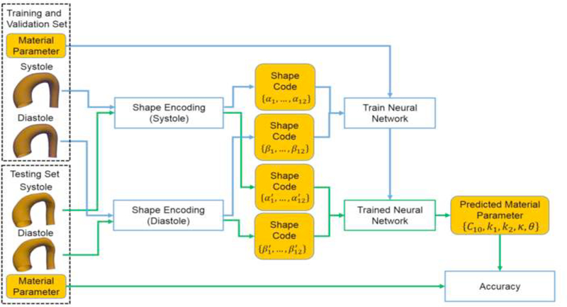
Evaluating the accuracy using the testing dataset.

3. RESULTS

Given a pair of geometries as the inputs, the trained ML-model can output the material parameters within one second on a PC with 3.6GHz quad core CPU and 32GB RAM. The actual versus predicted material parameters in the testing set are shown in Figure 9. The ranges of material parameters are resulted from the convex hull in Section 2.2.1, similar ranges of material parameters were reported in the studies [47, 48], which were obtained by fitting the GOH model to uniaxial testing data.

Figure 9.

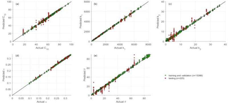
The actual and predicted material parameters. Each point was plotted using its actual value as horizontal x-coordinate and the ML-predicted value as the vertical y- coordinate. A perfect straight line (y=x) indicates perfect prediction, and any deviation from the straight line indicates prediction errors.

We define the normalized standard deviation of absolute error (NSTAE) of the k^th material parameter as

$$NSTA{E}_k=\frac{1}{\left({\max }_l\left(y_k^{(l)}\right)-{\min }_l\left(y_k^{(l)}\right)\right)}\sqrt{\frac{\sum _{l=1}^N{\left(A{E}_k^{(l)}-{\overline{AE}}_k\right)}^2}{N-1}}\times 100\%$$ (20)

where $\overline{A{E}_k}$ is the averaged absolute error for the k^th material parameter. The NMAE and NSTAE for each material parameter in the testing set are reported in Table 3. The errors indicate that the ML-predicted material parameters are in good agreement with the actual material parameters.

Table 3.

NMAE and NSTAE of the five material parameters in testing set (10,000 epochs).

	C10	k1	k2	К	θ
NMAE	3.75%	1.38%	6.01%	1.88%	3.74%
NSTAE	3.51%	1.59%	4.38%	1.89%	4.56%

The errors might be explained by coupling effect (over-parameterization) of the constitutive model [12], different combinations of material parameters may have similar stress-strain response. This nonlinear coupling has resulted in identification difficulties in the optimization-based inverse approaches [14, 15, 17],

To further evaluate the estimation results, stress-stretch curves were plotted by simulating stretch-controlled biaxial tension in MATLAB by assuming the tissue is loaded in the plane stress state and the material is incompressible. We use σ₁ and ${\lambda }_1$ to denote the circumferential stress and stretch, σ₂ and ${\lambda }_2$ to denote the longitudinal stress and stretch. The simulations were based on the following 3 protocols: (1) in the circumferential strip biaxial tension, fixing ${\lambda }_2=1$ while increasing ${\lambda }_1;$ (2) in the equi-biaxial tension, keeping the ratio ${\lambda }_1/{\lambda }_2=1;$ (3) in the longitudinal strip biaxial tension, fixing ${\lambda }_1=1$ while increasing ${\lambda }_2.$ In total, six stress-stretch curves are generated for each set of constitutive parameters.

Using the testing dataset, the coefficient of determination (R²) was calculated for each curve, and the averaged coefficient of determination of the six curves for each input-output pair was obtained. The predictions were sorted according to their averaged coefficient of determination. The best, median, worst cases are plotted in Figure 10, and the corresponding actual and predicted material parameters are shown in Table 4. Nearly matching agreement is achieved for the best cases. For the median case, although the discrepancies in the constitutive parameters seem obvious, the six curves still have close matches. In the worst case, the results are still acceptable in terms of material parameters, and the actual and predicted stress-stretch curves follow the same trends.

Figure 10.

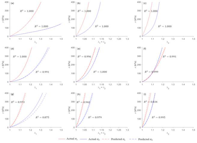
The actual and predicted stress-stretch curves for the best ((a), (b) and (c)), median ((d), (e) and (f)) and worst cases ((g), (h) and (i)).

Table 4.

The actual and predicted material parameters tor the best, median, worst cases.

		C10 (kPa)	k1(kPa)	k2	К	θ(°)
Best	Actual	63.83	1086.31	28.12	0.1553	7.76
	Predicted	64.66	1091.45	28.08	0.1561	7.55
Median	Actual	48.60	4207.03	4.76	0.2958	16.46
	Predicted	50.59	4325.85	2.20	0.2963	10.16
Worst	Actual	75.15	4683.21	17.53	0.2182	22.05
	Predicted	72.49	4485.17	19.48	0.2096	18.30

4. DISCUSSION

Optimization-based inverse methods [14, 15, 17, 21] have been extensively used for material parameter identification problems. These methods are computationally-expensive. Iterative computations limit the efficiency of these approaches, prohibiting their clinical applications. The proposed ML approach can fundamentally resolve the challenge on computation cost. The ML-model builds a direct linkage between the geometries and the material parameters, bypassing the iterative procedures. Once the ML-model is trained, it can be used to make predictions instantaneously and repeatedly, such that in vivo material parameter estimation on any patient in real-time can be possible. Although FE simulations are used to generate training, validation and testing datasets, which takes approximately 10 days in our exemplary application. It should be noted that a similar amount of time is required to find the optimal material parameters for a single patient using nonlinear optimization [14, 15], The proposed ML-model was evaluated using additional testing data, where minor discrepancies (with NMAE about 1% to 6%) were achieved between the actual and ML-predicted material parameters. The close match between the actual and predicted stress-stretch curves further demonstrates the ML model can predict material constitutive responses with high accuracy. As a rough comparison, the previous approaches [14, 15] achieved a similar accuracy with deviation from 0% to 6% in terms of material parameters using numerically-generated data. However, it is infeasible to perform a quantitative comparison among different inverse methods [14, 15, 17, 21] as different datasets were used.

We chose neural network for the ML-model because it is highly scalable: it can be configured with more layers and units to handle an increasingly large amount of data. Other ML-models can also be used for the material parameter identification problem. For instance, support vector regression (SVR) with radial basis function (RBF) kernel [49] can be applied to our datasets. Utilizing the v-SVR with fine-tuned parameters (C = 7,v = 0.5, γ = 0.3, definitions referring to [49]), we were able to predict the material parameters with similar accuracy as the neural network. As demonstrated in Table 5, the NMAEs of the SVR predictions are slightly higher than those of the neural network.

Table 5.

NMAE and NSTAE of the five material parameters in testing set using support vector regression (SVR).

	C10	k1	k2	К	θ
NMAE	4.53%	2.35%	5.16%	1.64%	4.26%
NSTAE	3.35%	2.07%	3.57%	1.57%	5.14%

Our proposed ML model is not tied to the particular form of the constitutive model (Eqn. (4)–(7)). As long as a constitutive model can be implemented in a FE package, it can be used to generate training and testing data. For example, more advanced fiber dispersion models [50–52] can be used in our future work to handle fiber tension-compression switch.

The applications of machine learning techniques on the complex inverse mechanics problems can be traced back to the 1990s [53], when neural networks were first introduced to traditional mechanics fields for constitutive modeling [54] and elastic-plastic fracture mechanics [55], The pioneering work by Huber and Tsakmakis [56, 57], determined certain constitutive parameters from the spherical indentation data using neural networks. Because this classical problem can be characterized by the load-depth trajectory, some manually selected features (e.g. depth at a given load level) were sufficient. However, to determine material parameters of the aortic wall from medical image data, the 3D geometrical information has to be fully exploited, which cannot be described by using a few intuitive features. In our ML-model, the PCA effectively encodes the input complex geometries into the shape codes. Next, a neural network (24 inputs - 256 hidden units - 256 hidden units - 5 output units) with softplus activation function was utilized to establish the nonlinear mapping between the shape codes and the material parameters. The comparison between the softplus units and other units is illustrated in Figure 11. The softplus units outperformed the conventional sigmoid and hyperbolic tangent (tanh) units, the ReLU [42] and its variant SELU [58], The softplus units lead to the lowest loss in the testing set and thus are more appropriate for this application.

Figure 11.

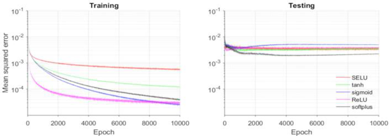
MSE loss function for training and testing using softplus and other units.

Since this study only aims to demonstrate the feasibility of the proposed machine learning framework, virtual aorta geometries were used for training and testing our ML-model. We acknowledge that the numerically-generated data may not represent the actual patient geometries and our ML-model has this limitation. Our current ML-model may not be able to handle complex situations such as calcifications in the aorta. The following assumptions and simplifications were used in data generation to expedite the FE simulations: (1) the branches of the aortic arch were trimmed off; (2) because of the partial volume effect [59], it is difficult to obtain the wall thickness from CT images, therefore, a uniform wall thickness at the systolic phase (1.5 mm) was assumed based on the average value from [38]; (3) the systolic and diastolic pressure were assumed to be 120mmHg and 80 mmHg, respectively for all cases; (4) to reduce model complexity, residual stresses were ignored according to a study [60] which shows that the residual stresses have minor effects on the material parameter identification problem; and (5) homogenously distribution of the material properties was assumed, while it is well known that aneurysms have heterogeneously distributed material properties. However, we note that these assumptions and simplifications were also present in the previous optimization-based inverse approaches [14, 15, 17, 21], The main advantage of the ML-based approach is that it can significantly reduce the computation time. These limitations can be resolved in future work. For examples, the branches can be re-meshed using existing mesh processing method [61], then encoded by additional shape codes. Using advanced MRI [62], the wall thickness may be measurable for individual patient. The full 3D geometries at the two cardiac phases can be encoded using PCA, and therefore the thickness field is naturally accommodated. To handle pressure variations, FE simulation data at a wide range of systolic and diastolic pressure levels can be generated, and the systolic and diastolic pressure can be included as two additional inputs to the neural network. To incorporate the residual stresses, a modified GPA algorithm [63] can be applied to generate training and testing datasets.

Although the feasibility of the ML-model is clearly shown, the model is not ready for clinical application yet until sufficient real patient geometries are available. When a substantial amount of medical image data and experimental testing data are obtained, we can update the SSM space and the convex hull, from which a new large training dataset can be generated using the framework proposed in this study. The updated ML-model will be capable of predicting the material parameters which may provide clinically relevant insights, i.e. serving as a basis for patient-specific rupture risk estimation [37], In case of a new patient with extreme aorta shape or material properties, which may cause unreliable prediction, a rejection option can be added in the ML-model as in [64], The enhanced ML-model may avoid making predictions on uncommon cases. Those rare cases can be handled by the optimization-based inverse methods [14, 15, 17, 21].

5. CONCLUSION

We have proposed a novel ML approach to estimate the constitutive parameters of the aortic wall from in vivo loaded geometries at two cardiac phases with known blood pressures. The ML-model is comprised of an unsupervised shape encoding module and a supervised nonlinear mapping module. FE simulations were used to generate datasets for training, adjusting and testing the ML-model. This novel ML approach can expedite the procedure of in vivo material parameter identification: once the ML-model is trained, the material parameters can be estimated within one second.