Analyzing DNA Methylation patterns during tumor evolution

Abstract

Epigenetic modifications play a key role in cell development and tumorigenesis. Recent large-scale genomic studies have shown that mutations in the epigenetic machinery and concomitant perturbation of epigenomic patterning are frequent events in tumors. Among all the epigenetic marks, DNA methylation is one of the most studied. Hyper/hypo-methylations on specific regulatory elements are sometimes thought to be correlated with expression of nearby genes. High-throughput bisulfite converted sequencing is currently the technology of choice for studying DNA methylation in base-pair resolution and whole-genome scale. Such broad and high-resolution coverage of the epigenome provide unprecedented opportunities to analyze DNA methylation patterns correlated with tumorigenesis and tumor evolution and progression. However, few pipelines are available to the public to perform systematically DNA methylation analysis. Here, utilizing open source tools, we describe a comprehensive computational methodology to thoroughly analyze DNA methylation patterns during tumor evolution based on bisulfite converted sequencing data, including intra-tumor methylation heterogeneity.

1. Introduction

Epigenetic modification plays a key role in the regulation of all DNA-based processes including transcription, DNA repair and replication, which are fundamental to tumorigenesis[1]. Recent large-scale genomic studies have shown that mutations in the epigenetic machinery and concomitant perturbation of epigenomic patterning are frequent events in tumors, such as B-cell lymphomas[2]. Among all known epigenetic modifications, DNA methylation is one of the most studied epigenetic markers. DNA methylation consists of the addition of a methyl group to carbon 5 of cytosine within the dinucleotide CpGs. Hyper- or hypo-methylation of genomic regions (promoters or enhancers for example) can lead to repression or activation of nearby gene expression. Several examples of promoter methylation levels inversely correlated with gene expression levels have been identified[3], frequently involving tumor suppressor genes. Thus, identifying differentially methylated cytosines (DMCs) and differentially methylated regions (DMRs), especially for those perturbed in tumors, has become a central point in cancer methylome analysis.

The advent of high-throughput DNA sequencing technologies has provided new opportunities to study DNA methylation, allowing for fast, single base resolution scans in targeted or enriched regions or at the whole-genome scale. Large-scale sequencing projects have generated hundreds of methylation profiles of tumors of different origins and at different stages. In turn, markers based on methylation usually provide important information about cellular phenotypes in normal and disease tissues and in many cases enable improved patient stratification over other approaches based on transcriptomics or mutation profiles. Enhanced reduced representation bisulfite sequencing (ERRBS) is one of such powerful high-throughput sequencing platforms, which can provide high sequencing depth and coverage of millions of CpGs in the human genome [4]. To date, few bisulfite sequencing analysis pipelines exist, even though such data are increasingly widely used. Here, we describe a comprehensive DNA methylation profiling analysis based on ERRBS data. This method is also applicable to reduced representation bisulfite sequencing (RRBS) data or whole-genome bisulfite sequencing (WGBS) data[5]. We focus our analysis on DNA methylation patterns during tumor evolution.

Following generation of an ERRBS data set, a typical analysis workflow consists of first identifying DMCs and DMRs, then correlating those regions to biological relevant genes and pathways. Other analyses relevant to tumor evolution may include quantifying intra-tumor methylation heterogeneity (MH). Indeed, comparing to the genetic code, DNA methylation is more flexible and cells within a cell population may have distinct methylation patterns. Thus a tumor cell population may harbor varying levels intra-tumor MH. Such heterogeneity is emerging as a powerful predictor of tumor evolution, progression and relapse[6]. The analysis of DNA methylation patterns during tumor evolution requires ERRBS samples from different tumor development stages, or at least diagnosis-relapse sample pairs from several patients. Also, ERRBS samples from normal tissues to be used as baseline can further enhance the analysis. The computational analysis scheme is outlined in Figure 1. Sample preparation and high-through sequencing are described there [4]. Sequencing reads from every stage during tumor evolution are mapped independently to a bisulfite converted reference genome, generating separate DNA methylation profile. DNA methylation status for every single CpG is determined in each sample, separately. Next, DMCs and DMRs calling is performed between the normal sample and each tumor stage or between any two tumor stages. Intra-tumor MH analysis is performed as a separate analysis on the same samples. Finally, identified DMCs/DMRs and MH hotspots are analyzed for enriched gene functions, in order to unravel pathways relevant to tumor evolution.

Figure 1.

Schematic of ERRBS data analysis pipelines.

2. Software

1. ERRBS data quality control: FastQC (available at http://www.bioinformatics.babraham.ac.uk/projects/fastqc/)[7].

2. Adaptive quality and adapter trimming: Trim Galore (available at http://www.bioinformatics.babraham.ac.uk/projects/trim_galore/)[8].

3. Bisulfite converted sequence reads mapping and cytosine methylation states calling: Bismark (available at http://www.bioinformatics.babraham.ac.uk/projects/bismark/)[9].

4. DMCs and DMRs calling: RRBSseeqer (available at http://icb.med.cornell.edu/wiki/index.php/Elementolab/)[6].

5. Regions annotations: ChIPseeqer (available at http://icb.med.cornell.edu/wiki/index.php/Elementolab/)[10].

6. Pathway analysis: iPAGE (available at http://icb.med.cornell.edu/wiki/index.php/Elementolab/)[11].

7. ERRBS data analyzing tools: Methylation heterogeneity analysis: errbs-tools including methylCall_from_Bismark.py, regionEpi.R and regionMH.R (available at https://github.com/SpursHeng90/errbs-tools/)[6].

3. Methods

1. Quality control for ERRBS reads

Similar to other high-throughput sequencing technologies, ERRBS is prone to systematic errors and artifacts such as PCR duplicates, GC-content shift and adaptor contamination. In addition to these common problems, ERRBS data can suffer more critical problems such as erroneous methylation status of cytosine introduced by end-repair and low bisulfite conversion rates. Thus, it is always a good idea to perform some simply quality control analysis to avoid any biases that may affect subsequent analyses. ERRBS generate output in FASTQ format, like most high throughput sequencing assays. We have successfully used a publicly available tool--FastQC--to address the quality control problem (Figure 1). Details about how to interpret the FastQC results are available in S. Andrews paper[7]. In general, per base sequence quality should be higher than cutoff (20 in most cases). Also, average per sequence quality should be around 38 (Phred+33, 0–41 scale). The other important feature is there is no overrepresented sequences or adapter contents, which can be potential adapter contamination sources. Ideally, your data set should pass most quality control steps to confirm the data quality for downstream analysis.

General syntax:

$ fastqc [-o output dir] [-f fastq|bam|sam] seqfiles1 … seqfilesN

Example:

$ fastqc -o . -f fastq CLL_S101.RRBS.fq

2. Adapter trimming

Suboptimal adapter contamination may affect read mapping, leading to low mapping efficiencies and even result in incorrect mapping and/or unreliable methylation calling in ERRBS. Even worse, positions filled in during end-repair can introduce artifact methylation status in ERRBS. Also, due to the short size selected fragment size of the restriction endonuclease MspI, ERRBS libraries with longer size have more severe problems from all above sources. To address this problem, we used read trimmers such as trim_galore (Figure 1).

General syntax:

$ trim_galore [options] <filenames>

Example:

$ trim_galore --rrbs –adapter

TGAGATCGGAAGAGCGGTTCAGCAGGAATGCCGAGACCGATCTCGTATGC --output_dir . CLL_S101.RRBS.fq

where:

--a/--adapter specifies the adapter sequence.

TGAGATCGGAAGAGCGGTTCAGCAGGAATGCCGAGACCGATCTCGTATGC is the standard adapters for Illumina. If no sequence was supplied it will attempt to auto-detect the adapter which has been used (Illumina, Small RNA and Nextera standard adaptors would be used).

--rrbs specifies that input file was an MspI digested RRBS sample.

3. Map ERRBS reads to reference genome

Mapping ERRBS reads to a bisulfite converted genome presents many computational challenges. Alignments should allow for mismatches, especially for potential methylation sites.

Also, alignments should be unique considering the numerous possibilities combining all the methylation status in each read to avoid miscalling of methylation levels. Among all the publicly available mapping tools, we have chosen bismark[9] to map ERRBS reads. Before mapping ERRBS reads to the reference genome, we need prepare the genome to bisulfite converted versions, which can be used by bismark aligner. FASTA/FASTQ format files for genome reference need to be in the genome folder. After genome preparation, we can map ERRBS reads to human genome.

General Syntax:

$ bismark_genome_preparation [options] <path_to_genome_folder>

$ bismark [options] <genome_folder> {−1 <mates1> −2 <mates2> | <singles>}

Example:

$ bismark_genome_preparation <genome_folder>

$ bismark -l 29 --bowtie1 --multicore 6 GRCh37 --output_dir . CLL_S101.RRBS_trimmed.fq

where:

-I specifies the “seed length”, which is the number of bases of the high quality end of the read. Typically, the length of sequencing reads can be used here.

--bowtie1 specifies that bismark will create indexes for bowtie 1[12].

--multicore sets the number of parallel instances of bismark to be run concurrently.

--output_dir specifies that all output files are written into this directory.

4. Cytosine methylation state calling

Once suitable ERRBS alignments are generated, methylation status for individual sites (mostly CpG sites) can be determined. To be consistent with our alignment processes, we utilize a simple script from bismark to achieve this goal.

General Syntax:

$ bismark_methylation_extractor [options] <filenames>

Example:

$ bismark_methylation_extractor -s --output . --merge_non_CpG --multicore 6 -- genome_folder <genome_folder> CLL_S101.RRBS_trimmed.fq_bismark.bam

Typically, we need to extract methylation status from those two files:

CpG_OT_CLL_S101.RRBS_trimmed.1bp.fq_bismark.txt and

CpG_OB_CLL_S101.RRBS_trimmed.1bp.fq_bismark.txt. All the reads in files labeled with OT reflect methylation levels of CpGs in forward strand and all the reads in files labeled with OB contain methylation information of CpGs on reverse strand. For the methylation state, “+” and “-” indicate methylated and unmethylated CpGs, respectively. In accordance with this label, “Z” and “z” represent methylation and unmethylated CpGs. Those two labels should agree with each other. After this step, it’s usually important to check the general features of the bismark outputs for all of your samples, such as mapping efficiency, average conversion rate, number of CpGs, average coverage and average CpG methylation levels (Table 1). One of the most important features is average conversion rate, which detects how bisulfite treatment can convert unmethylated Cytosine successfully. This number is usually higher than 99.7% (Table 1). More over, samples should have acceptable mapping efficiency (60% or higher), which varies according to sequencing read length. Also, samples analyzed together should ideally have similar covered CpGs, similar average coverage across the whole data set and similar average CpG methylation levels in each category/group. For example, tumor samples have similar higher average CpG methylation levels versus normal samples (Table 1).

Table 1 –

Bismark output statistics example.

id	#reads	mapping efficiency	average coversion rate	#CpGs(10X)	average coverage	average CpG methylation levels(%)
1	73293324	64.50%	99.8979	2848900	51.82	34.40%
2	76101498	66.00%	99.8947	2933770	50.14	31.50%
3	85482964	66.50%	99.8838	2822016	56.84	39.50%
4	80272372	66.50%	99.8138	2795046	56.97	35.90%
5	64361288	66.60%	99.7396	2625874	50.8	34.50%
6	78897537	66.90%	99.8999	2782944	56.52	33.80%
7	76009876	66.00%	99.8751	2850695	52.66	38.20%
8	75431630	65.90%	99.778	2893682	52.82	38.40%
9	76653335	65.20%	99.8868	2843240	54.8	39.00%
10	78481481	65.00%	99.8859	2808703	54.04	38.50%
11	73287618	67.60%	99.8617	2733715	52.24	37.20%
12	73847281	67.50%	99.7764	2920328	50.99	36.50%
13	81504963	66.30%	99.8747	2822336	58.31	41.90%
14	96892822	62.50%	99.8899	2795175	59.89	48.80%
15	43137414	64.20%	99.8866	1609370	48.55	30.80%
16	72217478	66.50%	99.7681	2741285	54.08	45.90%
17	72922475	66.90%	99.8376	2872522	53.3	38.20%
18	75434628	66.80%	99.8349	2839250	52.93	38.30%
19	73437411	66.30%	99.8747	2767916	52.07	39.10%
20	82936367	68.00%	99.8547	2823987	52.74	36.10%

5. Data format transformation

This tutorial uses RRBSeeqer to call differentially methylated cytosines and regions. We thus need to convert bismark output files into a format that can be read by RRBSeeqer (Methyl files, Table 2).

Table 2 –

RRBSeeqer input files example.

chrBase	chr	base	strand	coverage	freqC	freqT
chr1.10542	chr1	10542	F	587	99.83	0.17
chr1.10636	chr1	10636	F	57	85.96	14.04
chr1.10617	chr1	10617	F	58	100	0
chr1.10589	chr1	10589	F	58	100	0
chr1.10631	chr1	10631	F	56	100	0
chr1.10638	chr1	10638	F	57	85.96	14.04
chr1.10609	chr1	10609	F	58	98.28	1.72
chr1.10620	chr1	10620	F	59	93.22	6.78
chr1.10525	chr1	10525	F	609	95.24	4.76
chr1.10497	chr1	10497	F	606	97.85	2.15
chr1.10633	chr1	10633	F	58	89.66	10.34
chr1.133181	chr1	133181	R	118	61.02	38.98
chr1.133218	chr1	133218	R	117	54.7	45.3
chr1.133180	chr1	133180	F	131	40.46	59.54
chr1.133165	chr1	133165	F	136	88.24	11.76
chr1.135028	chr1	135028	F	168	88.1	11.9
chr1.135203	chr1	135203	R	77	87.01	12.99
chr1.135208	chr1	135208	R	77	90.91	9.09
chr1.135173	chr1	135173	R	78	87.18	12.82
chr1.134999	chr1	134999	F	170	31.18	68.82
chr1.135191	chr1	135191	R	76	94.74	5.26
chr1.135179	chr1	135179	R	79	67.09	32.91
chr1.135031	chr1	135031	F	168	90.48	9.52
chr1.135218	chr1	135218	R	71	78.87	21.13
chr1.136911	chr1	136911	F	103	92.23	7.77
chr1.136913	chr1	136913	F	101	94.06	5.94
chr1.136895	chr1	136895	F	104	67.31	32.69
chr1.136876	chr1	136876	F	104	95.19	4.81
chr1.136925	chr1	136925	F	103	0.97	99.03
chr1.137120	chr1	137120	F	29	96.55	3.45
chr1.137157	chr1	137157	F	29	100	0
chr1.137169	chr1	137169	F	28	0	100
chr1.139059	chr1	139059	F	13	0	100
chr1.139029	chr1	139029	F	13	61.54	38.46
chr1.139073	chr1	139073	F	13	61.54	38.46
chr1.237094	chr1	237094	F	99	7.07	92.93
chr1.249382	chr1	249382	R	29	0	100
chr1.249429	chr1	249429	R	29	93.1	6.9
chr1.531247	chr1	531247	R	29	100	0
chr1.531265	chr1	531265	R	29	100	0

General Syntax:

$ python methylCall_from_Bismark.py [options] <sample_name> <input_dir> <output_dir>

$ perl epicore2calls.pl <input_file> | gzip > <output_file>

Example:

$ python methylCall_from_Bismark.py -c 10 CLL_S101 bismark_output/ cpg/

$ perl epicore2calls.pl cpg.CLL_S101.mincov10.txt | gzip > cpg.CLL_S101.mincov10.txt.calls.gz

where:

-c specifies the minimum coverage required per CpG site for downstream analysis.

6. DMRs identification patient-by-patient

Identifying DMRs is one of the most important problems in DNA methylation analysis. DMCs and DMRs typically reflect local DNA methylation changes during tumor evolution, such as those occurring in tumors between diagnosis and relapse. Several methods enable discovery of consistently hypo- or hyper-methylated cytosines or regions across several samples. We and other groups have observed significant inter-patient MH in diffuse large b-cell lymphomas (DLBCL), a prevalent non-Hodgkin lymphoma. Hence, we have sought to define DMCs and DMRs on a patient-by-patient basis. We used our in-house tools—RRBSseeqer—to extract DMCs and DMRs within individual patients. In general, we define DMCs using RRBSseeqer_CG followed by a serial of file passing steps (false discovery rate=20%, Chi-square tests). Next, DMRs were defined as regions containing at least five DMCs and whose total methylation difference was more than 10%. The use of five or more DMCs partially overcomes the statistical limitation of individual Chi-square tests based on n=1 patients sample. As the output, we will get DMR files with a single DMR per row including chromosome, start position, end position, size, number of CpGs in DMR and methylation difference.

General Syntax:

$ RRBSseeqer_CG -rrbs1 <control_file> -rrbs2 <experiment_file> | sort_column.pl | sort_column_alpnum.pl > <output_file>

$ Perl RRBSidentifyUpDownDMR.pl --metfile=<input_file> --outfile=<output_file> [options]

Example:

$ RRBSseeqer_CG -rrbs1 cpg.normal.mincov10.txt.calls.gz -rrbs2 cpg.CLL_S101.mincov10.txt.calls.gz -test chi | sort_column.pl 1 | sort_column_alpnum.pl 0 > DMC.CLL_S101.txt

$ perl RRBSidentifyUpDownDMR.pl --metfile=DMC.CLL_S101.txt --dmax=250 -- minmetdx=0.1 --minnumcg=5 –outfile=DMR.CLL_S101.txt

where:

-rrbs1 should be normal samples or earlier tumor stage samples.

-rrbs2 should be tumor samples or later tumor stage samples.

-dmax specifies the largest distance between two DMCs.

-minmetdx specifies the minimum average DNA methylation difference to detect a valid DMR.

-minnumcg specifies the minimum number of DMCs needed to detect a valid DMR.

7. Unsupervised analysis of pathways over-represent in tumor samples

To explore DMRs between Diagnosis and Relapse samples for each patient further, we need to annotate each DMR with the closest gene. We then perform pathway analysis to identify gene sets and pathways over-represented within the DMR associated genes in each patient. Generally, we annotate DMRs to different genomic locations with ChIPseeqerAnnotate from ChIPseeqer. First, we use ChIPseeqerAnnotate to annotate DMRs to genomic locations based on hg19 human genome and RefSeq gene annotations. Then, DMRs overlapped with promoters (defined as ± 2kb windows centered on RefSeq transcription start site) are extracted and converted to iPAGE acceptable file format). The last step is running pathway analysis against known pathways in GO[13]. The outputs list over- or under-representation levels in log10 P values. We then perform unsupervised analysis of genes or pathways can give us a sense how methylation perturbation in each patient compares to each other (Figure 2a).

Figure 2. Examples of DMRs identification and visualization.

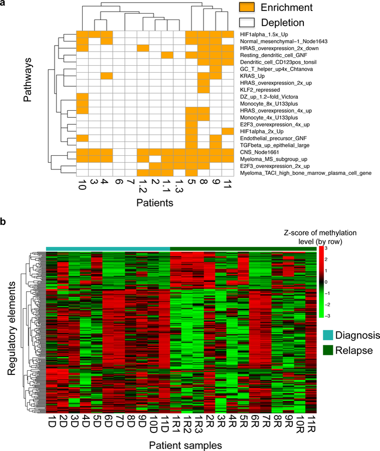
(a) Pathways overexpressed with hypermethylated genes (promoters overlapped with hypermethylation DMRs) of individual patients were illustrated here. Each row represents a single pathway and each column represents a patient pair. (b) Each row represent single differentially methylated regulatory element. Each column represent single diagnosis/relapsed sample from patients. Scale bar represent z-score of methylation level. Values were centered and scaled in row direction.

General Syntax:

$ ChIPseeqerAnnotate --peakfile=<input_file> [options]

$ mergeCSAnnotateGenesColumns.pl --genefile=<input_file> --outfile=<output_file> [options]

$ make_PAGE_input.pl --geneslist=<input_file> [options]

$ page.pl –expfile=<input_file> [options]

Example:

$ ChIPseeqerAnnotate --peakfile=DMR.CLL_S101.txt --genome=hg19 --db=refSeq

$ mergeCSAnnotateGenesColumns.pl -- genefile=DMR.CLL_S101.txt.refSeq.GP.genes.annotated.txt --geneparts=P --showORF=1 -

-outfile=DMR.CLL_S101.pro.txt

$ make_PAGE_input.pl --geneslist=DMR.CLL_S101.pro.txt --refgene=/data/hg19/refSeq

$ page.pl –expfile=DMR.CLL_S101.pro.txt.ORF.txt --pathways=human_go_orf -- cattypes=P,C,F -suffix=GO

where:

--genome specifies using hg19 as reference genome.

--db sepecies using RefSeq gene as gene annotation.

--pathways sets known pathways in GO.

--cattypes specifies using molecular function (F), cellular component (C) and biological process (P) parts of GO.

8. Supervised analysis to call DMRs across all the patients

An alternative way to DMRs patient-by-patient analysis is to directly call DMRs across all the patients. Unlike unbiased DMRs, we selected the region boundaries in this type of analysis, promoter or CpG Islands for example. Enhancers and other methylation sensitivity regulatory elements are also good candidates, such as CTCF binding sites. The methylation level for each region in each sample is calculated by averaging the methylation levels of all CpGs (at least 5 CpGs) inside the corresponding regions.

General Syntax:

$R CMD BATCH --no-save --no-restore [options] regionMethyl.R regionMethyl.log

Example:

$R CMD BATCH --no-save --no-restore ‘--args input_dir=cpg/ output_dir=. regions=promoter22kb.rds regionMethyl.R regionMethyl.log

where:

--no-save specifies that nothing will be saved in the .Rdata file.

--no-restore specifies that R does not read the .Rdata file in the current directory.

--args specifies arguments used from the rscript: input_dir sets the location of CpG Methyl files, all the outputs are written to output_dir, regions are promoter annotations (defined as ± 2kb windows centered on RefSeq transcription start site) in GenomicRanges data types[14], regionMethyl.R is the manuscript and regionMethyl.log is the output record of running this script with R.

This analysis generates a matrix with methylation levels for all the regions across all the samples. The next step is to call DMRs between two groups of samples. While there are several methods for calling DMRs, perhaps one of the simplest methods is to use paired T-test/Wilcox-test between diagnosis and relapse sample pairs followed by correction for multiple testing. A minimum methylation difference is also often used to ensure biological relevance of any significant change. Differentially methylated promoters across all the patients can be visualized using a heatmap (Figure 2b).

9. Intra-tumor MH characterization

It is common to use DMRs or average DNA methylation levels to characterize DNA methylation. However, DNA methylation is measured from cell population, from which methylation patterns are sampled. Bisulfite converted DNA reads may contain multiple CpGs thus enabling a per-read analysis of DNA methylation patterns. In such analyses, loci with identical average DNA methylation levels can have distinct DNA methylation patterns between samples. Such distinct patterns are the result of intra-tumor MH (Figure 3a). Intra-tumor MH has been connected to gene expression levels and to clinical outcome in several types of tumors such as chronic lymphocytic leukemia (CLL) and DLBCL. For example, higher MH are linked to lower gene expression levels in CLL and patients with higher MH levels at diagnosis stage in DLBCL have a higher chance to relapse after chemotherapy[6, 15]. The concept of epipolymorphism has been used to describe and quantify methylation heterogeneity [16]. The epipolymorphism level of a four-CpG locus (reads containing 4 or more contiguous CpGs) was defined as the probability that epialleles randomly sampled from the locus differ from each other. Higher epipolymorphism corresponds to higher intra-tumor methylation heterogeneity and vice-versa. Epipolymorphism can be analyzed at individual loci based on ERRBS data. A global epipolymorphism level can also be calculated. Briefly, epipolymorphism is calculated for each locus in a sample. Epipolymorphism is correlated with methylation level (with epipolymorphism being lowest at highest or lowest methylation levels), therefore global epipolymorphism must be normalized by methylation levels. Our global analysis divides loci into different bins depending on their methylation levels and median epipolymorphism is calculated for each bin. The area under the median line is defined as MH for each patient (Figure 3b–c). With this analysis, we can study the correlation between MH and tumor evolution.

Figure 3. Examples of intra-tumor MH analysis.

(a) Epipolymorphism levels are dependent on DNA methylation levels. All the loci were divided into different groups based on their methylation level and median epipolymorphism of each group is calculated. Genome-wide intra-tumour MH was quantified by area under the median line. (b) Median epipolymorphism lines for diagnosis and relapse tumors from patient 1.1 in our cohort. Intra-tumor MH visibly decreased with tumour evolution. (c) Relapsed samples displayed significant lower intra-tumour MH. All the loci located in gene promoter.

General Syntax:

$R CMD BATCH --no-save --no-restore [options] regionMH.R regionMH.log

Example:

$R CMD BATCH --no-save --no-restore ‘--args sample=CLL_S101 cpg_dir=cpg/ bam_dir=bam/ output_dir=. regions=promoter22kb.rds regionMH.R regionMH.log

where:

--no-save specifies that nothing will be saved in the .Rdata file.

--no-restore specifies that R does not read the .Rdata file in the current directory.

--args specifies arguments used from the rscript: sample sets the sample name, cpg_dir sets the location of CpG Methyl files, bam_dir sets the directory of bam files, all the outputs are written to output_dir, regions are promoter annotations (defined as ± 2kb windows centered on RefSeq transcription start site) in GenomicRanges data types[14], regionMH.R is the manuscript and regionMH.log is the output record of running this script with R.