Operational Local Join Count Statistics for Cluster Detection

Abstract

This paper operationalizes the idea of a local indicator of spatial association (LISA) for the situation where the variables of interest are binary. This yields a conditional version of a local join count statistic. The statistic is extended to a bivariate and multivariate context, with an explicit treatment of co-location. The approach provides an alternative to point pattern based statistics for situations where all potential locations of an event are available (e.g., all parcels in a city).

The statistics are implemented in the open source GeoDa software and yield maps of local clusters of binary variables, as well as co-location clusters of two (or more) binary variables. Empirical illustrations investigate local clusters of house sales in Detroit in 2013 and 2014, and urban design characteristics of Chicago census blocks in 2017.

1. Introduction

A large body of both empirical and methodological literature has expanded upon the use of local indicators of spatial association (LISA) since the original LISA framework was outlined in Anselin (1995, 1996), building upon the initial work by Getis and Ord (1992, 1996), and Ord and Getis (1995). Most of that research has focused on the situation where the variable of interest is continuous and considers statistics inspired by Moran’s I or Geary’s c.

Much less attention has been given to the case where the variable of interest is binary or categorical. A notable exception is the work of Boots (2003, 2006), where local indicators for categorical data (LICD) are proposed (see also Long et al. 2010). However, this work is situated in the context of regular lattice structures and does not readily generalize to irregular layouts. A slightly different perspective on a local join count statistic in both a univariate and bivariate setting is offered in Congdon (2016), where it is part of a hierarchical Bayesian specification for disease risk modeling, and not used in an exploratory sense.

In this paper, we consider the operational implementation of a local join count statistic, as a special case of a LISA. In the univariate case, we outline a local form of the so-called BB join count, i.e., where observations with a value of 1 occur in spatially adjacent locations, corresponding with positive spatial autocorrelation. While the material on the join count statistic is not particularly novel, our main contribution is to show how the univariate local join count statistic can been viewed as a constrained version of the local $G_i^{*}$ statistic of Getis and Ord (1992). We also extend the statistic to a bivariate and multivariate context, and differentiate between cases where co-location is possible and impossible. These statistics provide an alternative to the typical point pattern approach, for example, using a cross-K function (Ripley 1981), or a co-location quotient, such as the statistic proposed by Leslie and Kronenfeld (2011).

Our approach is appropriate in a data context where all potential locations are observed, i.e., a so-called lattice data structure. Specifically, this would be an exhaustive set of locations with both 0 and 1, such as all parcels in a city. This contrasts with a point pattern perspective, where only events are observed, and non-events are not, i.e., locations that might have had an event, but did not. A case-control setting provides yet another slightly different perspective in that non-events are represented by controls, but these typically do not exhaust all possible locations, so it is more akin to the point pattern setup than to the lattice data structure.

We are particularly interested in empirical contexts where the number of observations with a value of 1 is small relative to the sample size, i.e., uncommon (but not necessarily rare) events. We want to identify groups of locations where these events co-occur. In a spatially random setting, such co-occurrences would tend to be rare, hence identifying them provides a clue to “interesting” locations, in an exploratory sense.

In the remainder of the paper, we first outline the univariate local join count statistic, show its similarity to other statistics and discuss inference and interpretation. Next, we move to the bivariate context, and distinguish between the cases without and with co-location. We further extend the colocation cluster statistic to a multivariate setting.

We provide two empirical illustrations. In one, we use house sales locations in the City of Detroit for 2013 and 2014 to identify local clusters in each of the years, as well as clusters of sales in 2013 that are surrounded by clusters in 2014, as an application of a bivariate join count statistic without co-location. The second example investigates co-location clusters of Chicago census blocks that have been classified by means of urban design criteria as “Essential” (basic positive characteristics) and “Degrading” (negative, lack of walkability properties).

We close with some concluding comments.

2. A Local Join-Count Statistic

2.1. The Global Case

The general idea behind a LISA statistic as formulated in Anselin (1995) is that any global spatial autocorrelation statistic of the form Γ = ∑_i ∑_j f_ij can be decomposed into a collection of location-specific statistics of the form Γ_i = ∑_j f_ij for each location i. For binary variables, coded as 0 and 1, the global spatial autocorrelation statistic of choice is the join-count statistic (e.g. Cliff and Ord 1973). This statistic consists of counting the joins that correspond to occurrences of value pairs at neighboring locations. The three cases are joins of 1 – 1 (so-called BB joins, for ”black-black”), 0 – 0 (so-called WW joins, for ”white-white”), and 0 – 1 (so-called BW joins). The former two are indicators of positive spatial autocorrelation, the latter of negative spatial autocorrelation.

Since our interest lies in identifying co-occurrences of uncommon events, we focus on the BB join counts. More precisely, we consider the situation where the number of observations of 1 is much less than half of the sample (the definition of what is 1 or 0 can easily be reversed to make sure this condition is met). With the variable x_i at location i taking either the value of 1 or 0, a global BB join count statistic can be written as:

$$BB=\sum _i\sum _j{w}_{\mathit{ij}}{x}_i{x}_j,$$

where w_ij are the elements of a binary spatial weights matrix that specifies whether locations i and j are adjoining. Note that the latter is a perfectly general concept and does not need to be limited to strict contiguity. The definition of the spatial weights can encompass a wide range of neighbor definitions, such as k-nearest neighbors, distance bands, and even social network neighbors.¹ This form for the BB statistic can be seen to be a special case of the generalized spatial autocorrelation measures considered by Hubert et al. (1981), and is also the same as the numerator in the familiar Moran’s I (Moran 1948).

The global join count statistic also shows interesting similarities to a number of case-control statistics developed in a point pattern context. The logic behind these tests is to control for heterogeneous density by considering both cases (i.e., events of interest, such as the occurrence of a disease), and controls (i.e., locations that represent the spatial distribution of the population under consideration). Note the difference in the conceptualization of the space with the classic lattice context, where all locations are observed. In the case-control setup, the controls are usually a sample from the under-lying reference population.² The logic behind those statistics is to count the number of points surrounding a case and compare the frequency of cases to that of controls. A well-known example is the Cuzick-Edwards test, based on the k nearest neighbors of a case, i.e., T_k = ∑_i ∑_j a_ijδ_iδ_j (Cuzick and Edwards 1990, p. 77, Equation 5), where a_ij is based on a k-nearest neighbor relation, and δ_i,j = 1 for a case and = 0 for a control. Formally, this is identical to the BB join count statistic, except for the case-control setup. The Cuzick-Edwards test is further extended in Rogerson (2006) to counting the case-control frequency within a Thiessen polygon surrounding cases or within a given distance band. Again, the global statistic is formally equivalent to a join count statistic.³ Other statistics in the same case-control design, but also including the time dimension, are the so-called Q statistics introduced in Jacquez et al. (2005) (see also Jacquez et al. 2006, Jirjies et al. 2016). Similar to Cuzick-Edwards and Rogerson, these statistics count the number of cases among the k-nearest neighbors surrounding a case. The Q statistics also have a local counterpart.

A final set of global statistics that show a similarity to the join count statistic are the nonparametric tests based on symbolic analysis outlined in Farber et al. (2015) (see also López et al. 2010, Ruiz et al. 2010, for similar ideas). With similarity between two observations coded as a binary variable, this statistic again consists of counting the number of neighbors that are similar. However, the focus in these papers is on a global approach as an alternative to parametric test statistics, and not on detecting local clusters.

2.2. The Local Case

Following Anselin (1995), a local version of the BB statistic is:

$$B{B}_i=x_i\sum _j{w}_{ij}{x}_j.$$ (1)

Upon closer examination, with a binary spatial weights matrix, this boils down to a count of the neighbors with an observation of x_j = 1 for those locations where x_i = 1. For all locations with x_i = 0, the statistic is zero.⁴ Hence, the local join count statistic is only meaningful to assess whether locations with an “event” (i.e., x_i = 1) are surrounded by more other locations with events than would be the case under spatial randomness.

The local join count statistic as defined in Equation 1 is similar in spirit to the local second order analysis for point patterns outlined in Getis (1984) and Getis and Franklin (1987), where the number of points are counted within a given distance d of an observed point (see also Okabe et al. 2010, for further discussion and extensions). The distance cut-off d could readily form the basis for the construction of the spatial weights w_ij, which yields the join count statistic as a count of events (points) within the critical distance from a given point (x_i = 1). The main difference between the two concepts is the underlying data structure: in the point pattern perspective, the locations themselves are considered to be random, whereas the local join count statistic is based on a lattice perspective. The latter considers a finite set of known locations, for which both events (x_i = 1) and non-events (x_i = 0) are observed. In point patterns analysis, one does not know the locations where events might have happened, but did not.

In addition, except for a scaling factor, the local join count statistic also has the same structure as the local $G_i^{*}$ statistic of Getis and Ord (1992), when applied to binary observations (and with a binary weights matrix). The typical implementation of the local $G_i^{*}$ statistics is as:

$$G_i^{*}=\frac{{\sum }_j{w}_{ij}{x}_j}{{\sum }_j{x}_j},$$

where the sum in the denominator includes x_i The latter sum is therefore a constant scaling factor and can be ignored. The difference between the two statistics is that the local $G_i^{*}$ counts the neighbors with x_j = 1 for all locations, including the ones where x_i = 0. Such observations are ignored in the computation of the local join count statistic as outlined above. In a sense, the local join count statistic could thus be considered a constrained form of the local $G_i^{*}$, limited to observations where x_i = 1.⁵

2.3. Inference and Interpretation

Assessing the statistical significance of any local spatial autocorrelation statistic is fraught with problems, such as multiple comparisons and the potentially biasing effect of global spatial autocorrelation (for extensive discussions, see, e.g., Ord and Getis 2001, de Castro and Singer 2006, Rogerson 2015, Anselin 2018). As argued in Anselin (2018), rather than focusing on trying to obtain precise estimates of significance (which may be an unattainable goal), it may be more important to attempt to identify interesting observations, following the argument made by Efron and Hastie (2016).

This may constitute a problem when the size of the data set is large and the number of events is small. In such an instance, any occurrence of a rare event surrounded by another event is likely to be so exceptional that it automatically becomes “significant.” The interpretation of such clusters should be done with caution. They may be real, or they may be artifacts of the spatial scale of observation. In contrast to point pattern analysis, where the distance between points is unambiguous, the size of the areal unit typically varies considerably across a lattice data set and may introduce artifacts into the contiguity structure. As in any spatial autocorrelation statistic, the latter is crucial in determining meaningful neighbor relations.

Nevertheless, one can strive to quantify how likely a given pattern is to occur under a null hypothesis of spatial randomness. Two approaches can be taken. In one, the conditional probability of a configuration observed around a given location (i.e., with x_i = 1) can be computed, using the properties of a hypergeometric distribution.

Given a total number of events in the sample of N observations as P, we consider the number of neighbors of location i for which x_i = 1, i.e., conditional upon observing 1 at this location. The number of neighbors with x_j = 1 is represented by p_i. The probability of observing exactly p_i = p, conditional upon x_i = 1 follows the hypergeometric distribution for N − 1 data points and P − 1 events.⁶ The subtraction of 1 is due to the fact that x at i equals 1, and thus should be excluded.⁷ Formally:

$$\text{Prob}[p_i=p|x_i=1]=\frac{\left(\begin{array}{c}P-1\\ p\end{array}\right)\left(\begin{array}{c}N-P-2\\ k_i-p\end{array}\right)}{\left(\begin{array}{c}N-1\\ k_i\end{array}\right)},$$

where k_i is the number of neighbors for observation i.

Note that this measure only addresses the so-called compositional or a-spatial characteristics of the pattern (following the terminology of Boots 2003, 2006). In other words, it focuses on how many of the neighbors have a value x_j = 1, but ignores where these non-zero values occur among the neighbor sites (what Boots 2006, refers to as the configuration). In Boots (2006), several approaches are proposed to analyze patterns on regular lattice structures. However, the proposed methods do not generalize to irregular spatial layouts.

One could be tempted to use the properties of the join count statistic to compute a mean and variance under the null, and use an asymptotic (normal) approximation of the resulting z statistic.⁸ However, this is problematic for a local statistic. For a global statistic, the normal approximation is based on the asymptotics of an increasing number of observations. The counterpart for a local statistic would be an increasing number of neighbors. This creates two problems. On the one hand, if the increasing number of neighbors are viewed from an increasing domain perspective (e.g., the logic underlying the statistical properties of local regression), then the notion of neighbors changes and breaks the logic behind the lattice approach. On the other hand, in an expanding domain view of asymptotics, the number of neighbors would increase (asymptotically), defeating the notion of a local test.⁹ Therefore, such asymptotic approximations are not pursued.

Instead, a more traditional conditional permutation procedure is followed to compute a pseudo p-value, in the usual fashion. It should be noted that this is not equivalent to the exact probability approach, which actually underestimates uncertainty. In practice, the permutation approach is to be preferred, since it does not require any parametric assumptions and is formulated as a classical one-sided hypothesis test against the null hypothesis of spatial randomness. In what follows, we only consider the conditional permutation approach.

2.3.1. Conditional Permutation Test

A conditional permutation test as proposed in Anselin (1995) to compute a pseudo p-value for the LISA statistics can be constructed in the usual way. The general principle, for those locations i where x_i = 1, is to carry out a series of random permutations of the remaining observations, while counting the times the number of neighbors with x_j = 1 equals or exceeds q_i, the observed value of the join counts. In practice, this is implemented by taking k_i (the number of neighbors for i) draws without replacement from a set of N − 1 observations with K − 1 values of 1 for those observations where x_i = 1. A pseudo p-value can be computed as (v + 1)/(r + 1), where v is the number of times the neighbors have q_i or more values equal 1, and r is the number of permutations. The standard caveats apply (e.g., sensitivity to the number of permutations, varying results depending on the random number sequence, multiple comparisons, etc.).

It should be noted that, as a one-sided test, the conditional permutation approach includes instances as rejecting the null of spatial randomness where there are more than q_i neighbors with x_j = 1 in the computation of the pseudo p-value.

3. Bivariate Local Join Count Statistics

In the bivariate case, we consider the co-occurrence or clustering of observations with values of 1 for two binary variables, say x and z. The bivariate case is more complex than a simple generalization of the univariate case, since the co-location of the events at i needs to be taken into account. The term co-location itself is somewhat confusing, since it sometimes relates to the simple occurrence of two events in the same place, and other times to the spatial relationship between two different types of events. Here, we focus on the latter.

The complexity of the bivariate case is also encountered when dealing with both the correlational and the spatial correlation aspects in a spatial autocorrelation statistic such as Moran’s I. For example, in the original implementation of the bivariate local Moran, described in Anselin et al. (2002), the correlational aspect is ignored. The original bivariate local Moran was defined as a measure of the strength of association between a variable x at i and its neighbors for a different variable z, but ignores any possible correlation between x and z at i. In the approach proposed by Lee (2001), the two aspects of the bivariate relationship are separated into a correlational part and a spatial correlational part. Alternatively, in Anselin (2018), the issue of in-place correlation is side-stepped by using a metric of squared distance in attribute space, as a generalization of Geary’s c.

The spatial clustering of two different events has received considerable attention in the point pattern literature. The classic measure is Ripley’s cross-K function (Ripley 1981), which addresses the spatial correlation between two marked point patterns. Similar in spirit is the co-location quotient proposed by Leslie and Kronenfeld (2011), which exploits the distance ranks between adjoining marked point patterns (see also Leslie et al. 2012, Cromley et al. 2014, Mack et al. 2017, Wang et al. 2017, among others, for further details and applications).

Co-location is also an important topic of interest in the spatial data mining literature. For example, as defined by Huang et al. (2004, p.1472), colocation patterns “represent subsets of Boolean spatial features whose instances are often located in close geographic proximity.” In this context, Boolean spatial features are the “presence or absence of geographic object types at different locations.” However, the resulting methods, such as a the participation index proposed by Huang et al. (2004) are primarily designed to identify instances in large data bases where two features are closely located in geographic space. Instead, for a bivariate join count statistic those locations have already been identified, and the focus is on finding those observations where such an occurrence is a “significant” departure from spatial randomness.

In the discussion that follows, we continue to deal with a lattice data context and distinguish between two cases, one without in-situ co-location (i.e., co-location in i), and one with. As before, the analysis is conditional upon the values observed at location i.

3.1. No In-Situ Co-Location

The first case considers the situation where x_i and z_i do not take on the same value at i or j. In other words, when x_i = 1 for location i, then z_i = 0. We count the number of neighbors of i with x_i = 1 for which the value of z_j = 1 (and also x_j = 0).

This approach is useful when x and z cannot occur in the same location, such as when x and z correspond to two different values of a single categorical variable. For example, this would be the case when two different land uses for urban parcels are considered (e.g., when a parcel can only be classified as one land use category). However, it can also be used when x and z can co-locate, but do not. An example would be when observations are considered that fall in the same quantile for two different variables, but do not do so for a given location i. In general, we could consider the case where we are only interested in instances where the neighbor z_j = 1, irrespective of the value of x_j. However, this is less interesting from a substantive perspective. Instead, we focus only on the situation that satisfy the requirement that z_i = 0 when x_i = 1, and x_j = 0 when z_j = 1. The general form of the bivariate local join count (BJC) statistic is (allowing for all possible cases):

$$BJ{C}_i=x_i(1-z_i)\sum _j{w}_{ij}{z}_j(1-x_j)$$ (2)

The roles of x and z can be reversed, but the statistic is not symmetric, so the results may be different whether x or z is the focus.¹⁰

Note that when x_i ≠ z_i∀i, the term 1 − z_i = 1 for x_i = 1, and 1 − x_j = 1 for z_j = 1, so that the statistic can be simplified to:

$$BJ{C}_i=x_i\sum _j{w}_{ij}{z}_j$$ (3)

A pseudo p-value can be obtained from a one-sided conditional permutation test. This is implemented by carrying out a series of k_i draws for each location i where x_i = 1 and z_i = 0. The draws are without replacement from N − 1 data tuples (x_j, z_j) of which Q observations have z = 1 (since z_i = 0) and P − 1 observations have x = 1.¹¹ In practice, we only need to draw the z_j, since the matching x_j are zero by construction. The number of times the resulting local join count statistic from Equation 3 equals or exceeds the observed value yields a pseudo p-value.

3.2. Co-Location Cluster

A second perspective on the bivariate case is when the interest is in co-located events being surrounded by other co-located events.¹² We refer to this case as a co-location cluster (CLC). This requires both x_i = z_i = 1 as well as x_j = z_j = 1 for the neighbors. Formally:

$$CL{C}_i=x_i.z_i\sum _j{w}_{ij}{x}_j{z}_j$$ (4)

A conditional permutation approach can be constructed for those locations with x_i = z_i = 1. We draw k_i pairs of observations (x_j, z_j) from the set of N − 1 (this contains P − 1 observations with x_j = 1 and Q − 1 observations with z_j = 1). In a one-sided test, we again count the number of times the statistic in Equation 4 equals or exceeds the observed join count value at i.

3.3. Extension to More than Two Variables

The extension to multiple binary variables is mathematically straightforward, although maybe conceptually less so. While different combinations are possible, the most practical use case would be one where the interest focuses on the co-location of multiple variables coinciding with co-location for the neighbors. Again, we can refer to this as a co-location cluster. An example would be where binary variables were constructed from continuous-valued measures for those locations where the observations fall in a pre-specified range, such as the upper decile. The co-location cluster would indicate where such coincidences occur with neighbors that have similar coincidences. However, as the number of variables considered increases, we run into the “curse of dimensionality,” and results would be less and less meaningful, in the sense that such coincidences would likely be increasingly rare and thus always be indicated as “significant.”

Formally, we consider m variables at location i, i.e., x_hi for h = 1, …, m, with ${\prod }_{h=1}^m{x}_{hi}=1,$ i.e., conditional upon co-location of these variables at i. The corresponding co-location cluster statistic is then:

$$CL{C}_i={\prod }_{h=1}^m{x}_{hi}\sum _j{w}_{ij}{\prod }_{h=1}^m{x}_{hj}$$

The implementation of a conditional permutation strategy follows as a direct generalization of the bivariate co-location cluster. However, as pointed out, for a large number of variables, such co-locations become less and less likely, and a different conceptual framework may be more appropriate.

4. Empirical Illustrations

The univariate, bivariate, and multivariate local join count statistics were implemented in the latest version of the open source GeoDa software for spatial data exploration, available at http://geodacenter.github.io. The code is written in C++ and takes advantage of the built-in parallelization of current CPU hardware. In addition, it is also able to exploit the presence of graphics processing units (GPU) to speed up operations for large(r) data sets.

We illustrate the methods (and the software) with two empirical applications. In the first, we study local clusters of house sales in Detroit, MI, comparing the years 2013 and 2014. This uses the univariate local join counts for each year separately, and the bivariate (no co-location) local join counts to assess the degree of clustering of sales in 2014 around sales in 2013.¹³ This case illustrates the application of the local join counts as an alternative to point pattern statistics. The sales are represented as points (corresponding to the parcel centroids), but since we have all the parcel locations, we also have the observations where no sales occur, allowing for a lattice data approach.

In the second example, we utilize the classification of census blocks in Chicago, IL, using the urban design criteria outlined in Talen and Jeong (2018). We illustrate the co-location bivariate local join count statistic to assess the extent to which blocks classified as meeting “daily life essentials” (i.e., blocks containing one or more of grocery stores, day care center, library, senior center, neighborhood health clinic, farmer’s market or school) co-locate with blocks characterized as “degrading factors” (i.e., blocks having automotive facilities, parking lots, vacant lots or vacant buildings), and have this co-location for their neighbors as well. The potential clusters would suggest areas where planning intervention may be needed to enhance the positive life essentials aspects that are currently devalued by the degrading factors.

4.1. Clusters of House Sales in Detroit

Data on sales transactions in the Detroit housing market were obtained from the Detroit City Assessor’s office. For 2013 and 2014, the locations of the sales are associated with the centroid of the corresponding parcel. In this application, we do not consider the value of the sales, only the event as such.¹⁴

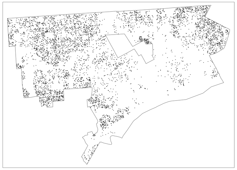
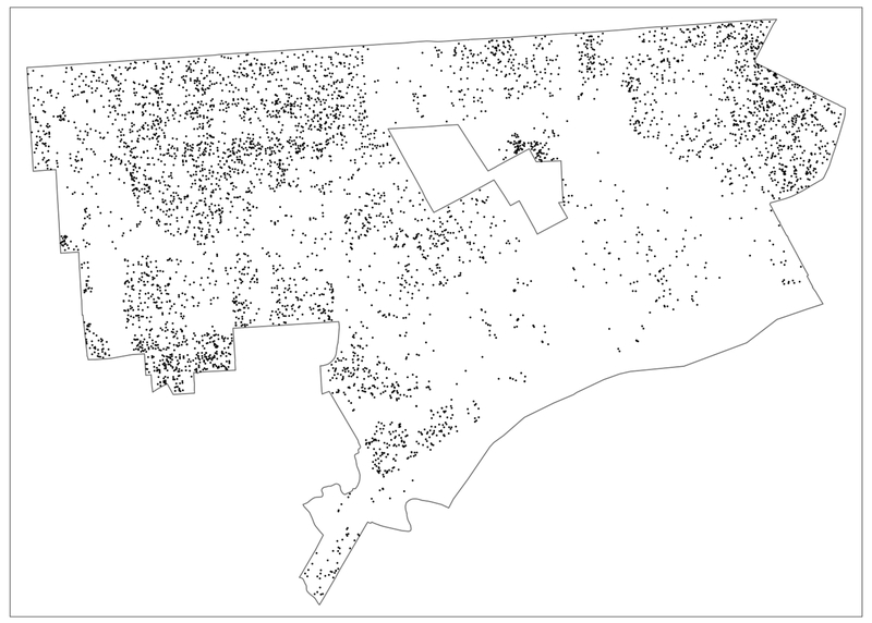
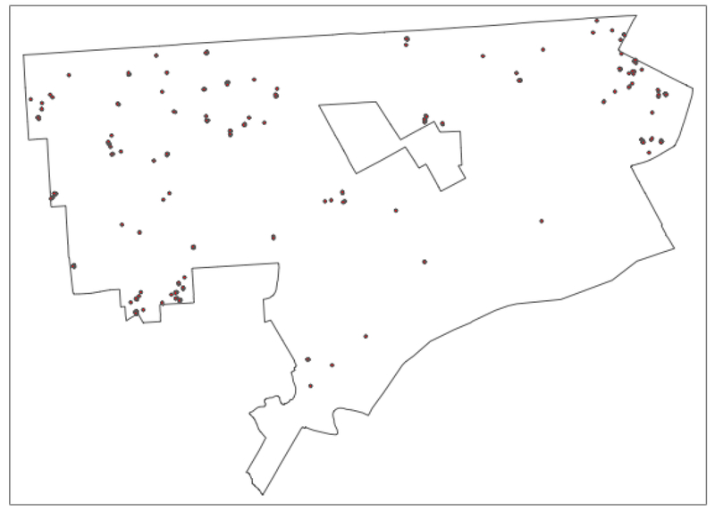
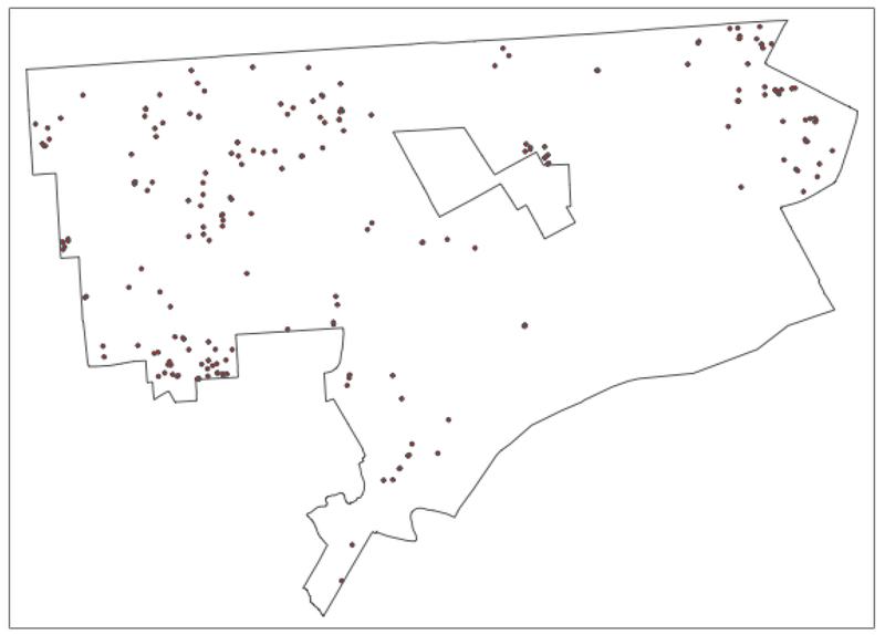
Our parcel data set consists of 384,396 observations. In 2013, there were 5,943 recorded sales transactions, and in 2014, there were 5,108. This represents respectively 1.5% and 1.3% of the total number of parcels. The point locations of the sales are shown in Figure 1 for 2013, and in Figure 2 for 2014. Since it is impractical to identify 384,396 parcels separately on a single map, only the transactions are shown.

Figure 1:

Point Locations of Detroit House Sales – 2013

Figure 2:

Point Locations of Detroit House Sales – 2014

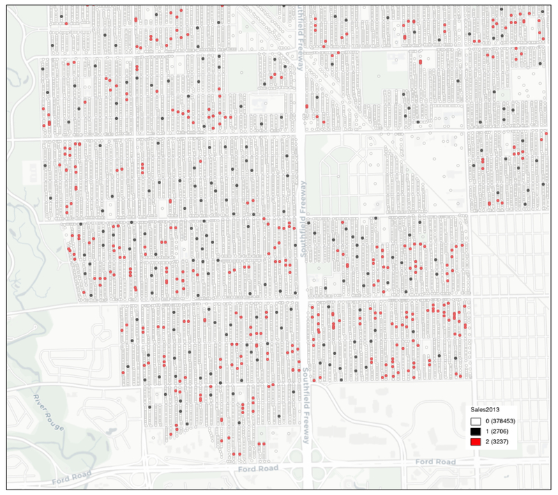
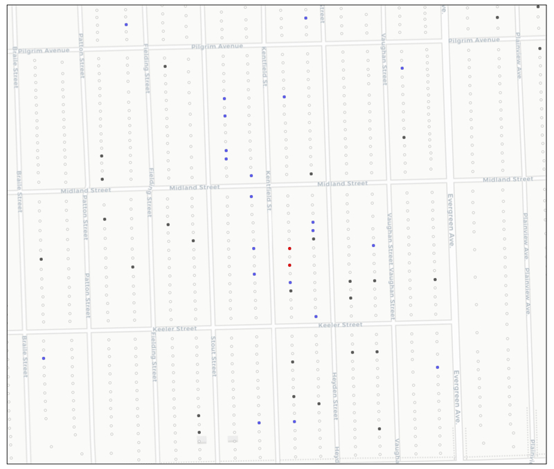
In order to gain a better appreciation of the spatial patterns involved, Figure 3 shows a close up image of a sub-area in the southwest corner of the city, close to River Rouge and the intersection of Ford Road and Southfield Freeway. The street pattern is included as a background. The empty outlines (white) are the parcel centroids without sales, the black dots have sales, and the red dots correspond to sales locations that also have sales among the neighbors (as defined below). Our goal is to identify those locations (red dots) where the number of neighbors with sales is greater than would be the case under spatial randomness.

Figure 3:

Sales Locations and Joins – 2013

(outline = no sales; black = sales, no neighbors; red = sales w neighbors)

A critical aspect of the local join count statistic is the definition of neighbors through the spatial weights matrix. For a large data set as the Detroit parcels with relatively few events, we need to make sure that the weights are meaningful, in the sense that the number of neighbors should adequately reflect the range of potential spatial spill-over. In our example, we used k-nearest neighbor binary spatial weights with k = 30.¹⁵ In terms of range, in both years, this represents an average maximum distance of 267 feet. The largest of these maximum distances is 916 ft in 2013, and 1095 ft in 2014. All are reasonable distances relative to the size of an average city block in Detroit (most blocks are roughly 250 ft by 800 ft). In other words, the 30 nearest neighbors correspond to the parcels in a block and one or two adjoining blocks (depending on the location of the parcel within the block).

A summary of the distribution of the number of neighbors with sales is given in Table 1. For each of the years, and also for the sales in 2014 surrounding sales in 2013, the cardinality of the neighbors is given. About half the sales do not have any other sales within the 30 nearest neighbor range. The largest number of nearest neighbors with sales is 6, obtained for one location in 2013, three locations in 2014, and two locations in 2013, surrounded by sales in 2014.

Table 1:

Cardinality of Nearest Neighbor Sales in Detroit

	2013	2014	2013-14
n	5943	5108	5943
0	2706	2586	3106
1	2032	1584	1871
2	844	664	707
3	274	196	192
4	79	61	52
5	7	14	13
6	1	3	2

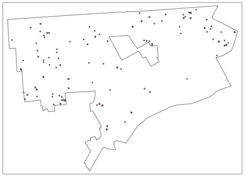
For each year, the univariate local join count statistics were computed, and their significance assessed with 999 permutations. The locations with a pseudo p-value of 0.01 or smaller are shown in Figures 4 and 5 (they are shown as points within the Detroit city boundary). In 2013, there were 188 such locations, and in 2014, there were 231.¹⁶ In terms of overall patterns, there seem to be some regions of similar clustering between the two years, especially in the western and north-eastern edges of the city.¹⁷

Figure 4:

Significant Univariate Local Join Count Locations – 2013

Figure 5:

Significant Univariate Local Join Count Locations – 2014

This overall pattern is also found for the bi-variate local join count statistic. In Figure 6, the locations with sales in 2013 surrounded by a significant cluster of 2014 sales are shown. Again, we used 999 permutations and a pseudo p-value of 0.01 or smaller. There are 214 such locations.

Figure 6:

Significant Bivariate Local Join Count Locations – 2013-14

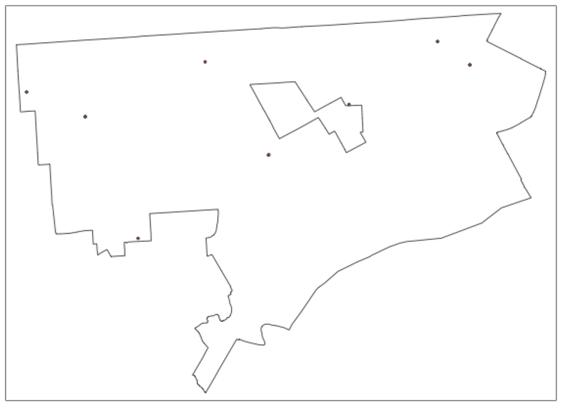
Finally, we find the locations of 2013 sales that form both a univariate local cluster and a bivariate local cluster, i.e., they are surrounded by other sales in both 2013 and in 2014. There are 11 such locations, depicted in Figure 7.¹⁸

Figure 7:

Locations Significant for Both Univariate and Bivariate Local Join Counts

In order to illustrate the type of spatial pattern that the identified clusters correspond with, we zoom in on two locations indicated as significant in both univariate and bivariate case (those two locations are shown as one point in the map in Figure 7). In Figure 8, we show those locations as red located on the same street block (they have one non-sales parcel in between them). They are surrounded by black dots, depicting sales in 2013, and blue dots, depicting sales in 2014, highlighting considerable activity in just a few adjoining blocks (the block sizes are 250 by 800 feet).

Figure 8:

Co-Location Hot Spot Close Up

4.2. Urban Design Characteristics of Chicago Census Blocks

In our final example, we illustrate the identification of co-location clusters using the bivariate local join count statistic. We use the classification of Chicago census blocks characterized as Essential and Degrading in Talen and Jeong (2018).¹⁹ If a block meets any of the criteria for this classification, it is coded 1, and 0 otherwise. As a result, each classification yields a 0–1 binary indicator variable. A block can be classified as meeting more than one category, so that the two indicator variables for Essential and Degrading can overlap. This provides a way to assess whether blocks that meet both criteria (note that the first is “good” and the second is “bad”) are surrounded by blocks that also meet both criteria, yielding spatial co-location clusters.

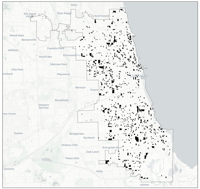
Of the 46,311 census blocks in Chicago, 1,803 are classified as meeting the Essential criteria, and 17,588 are categorized as Degrading. Figure 9 highlights the blocks that meet both criteria, i.e., blocks with co-location. There are 848 such blocks.

Figure 9:

Co-Location Map, Chicago Blocks with Essentials and Degrading

We define neighbors using the queen criterion for the census blocks. The resulting spatial weights matrix is extremely sparse, with only 0.02% non-zero cells. The median number of neighbors is seven.

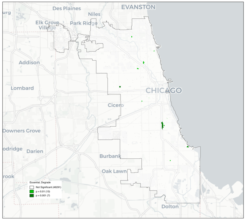
Again using 999 permutations, the bivariate local join count statistic indicates 20 locations as significant at a pseudo p-value of 0.01 or smaller. They are shown in Figure 10. Of the 20 locations, 7 are significant at 0.001, meaning (for 999 permutations) that none of the permuted data sets yielded a join count statistic equal to or higher than the observed one. They are shown in dark green on the map.

Figure 10:

Significant Co-Location Clusters, Chicago Blocks

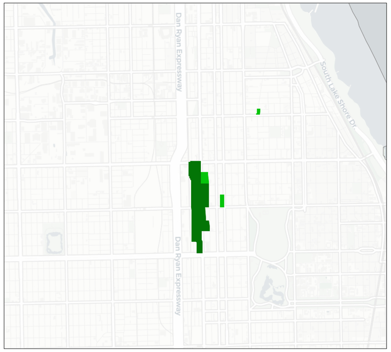
The largest cluster consists of five blocks in South Chicago, between 47th Street and Garfield Avenue, along State Street. These blocks are characterized by the presence of several educational institutions, but also contain many parking lots and other pedestrian unfriendly features that contribute to their classification as Degrading. A close up view in Figure 11 illustrates how the particular configuration of the blocks suggests a larger co-location cluster.²⁰ In terms of policy, these blocks could be considered prime candidates for remediation of some of the Degrading characteristics in order to enhance the Essentials.

Figure 11:

Co-Location Cluster Close Up

5. Concluding Remarks

In this paper, we proposed a number of local join count indices to detect spatial clusters. These form an alternative to point pattern statistics when the data context is such that both locations with and without events can be observed. The univariate statistic takes the form of a local BB join count and can be viewed as a constrained version of the familiar $G_i^{*}$ statistic.

The statistics are extended to a bivariate setting, distinguishing between a situation where co-location is not possible, and a situation where it is. For the latter case, we develop a co-location cluster statistic that can be readily generalized to a multivariate setting. However, as the number of variables under consideration increases, the curse of dimensionality leads to less and less useful results.

The statistics are implemented in the open source GeoDa software and applied in two empirical settings. In the first, univariate and bivariate local join counts (without co-location) are applied to house sales locations in Detroit. In the second, the bivariate co-location cluster test is applied to classifications of Chicago census blocks according to urban design criteria. In both applications, the results are intuitive and suggest interesting locations.

The methods outlined are exploratory, and should thus be applied with caution. We see them as a useful addition to the arsenal of the spatial data scientist for situations where the traditional local Moran and local Geary cannot be applied. The degree of complementarity with point pattern statistics, such as the cross-K, co-location quotients and case-control statistics, in situations where both are appropriate is the subject of future work.

References

- Akerlof GA (1997). Social distance and social decisions. Econometrica, 65:1005–1027. [Google Scholar]
- Anselin L (1995). Local indicators of spatial association — LISA. Geographical Analysis, 27:93–115. [Google Scholar]
- Anselin L (1996). The Moran scatterplot as an ESDA tool to assess local instability in spatial association In Fischer M, Scholten H, and Unwin D, editors, Spatial Analytical Perspectives on GIS in Environmental and Socio-Economic Sciences, pages 111–125. Taylor and Francis, London. [Google Scholar]
- Anselin L (2018). A local indicator of multivariate spatial association, extending Geary’s c. Geographical Analysis. doi: 10.111/gean.12164. [DOI] [Google Scholar]
- Anselin L and Rey SJ (2014). Modern Spatial Econometrics in Practice, A Guide to GeoDa, GeoDaSpace and PySAL. GeoDa Press, Chicago, IL. [Google Scholar]
- Anselin L, Syabri I, and Smirnov O (2002). Visualizing multivariate spatial correlation with dynamically linked windows. In Anselin L and Rey S, editors, New Tools for Spatial Data Analysis: Proceedings of the Specialist Meeting Center for Spatially Integrated Social Science (CSISS), University of California, Santa Barbara CD-ROM. [Google Scholar]
- Bavaud F (1998). Models for spatial weights: A systematic look. Geographical Analysis, 30:153–171. [Google Scholar]
- Boots B (2003). Developing local measures of spatial association for categorical data. Journal of Geographical Systems, 5:139–160. [Google Scholar]
- Boots B (2006). Local configuration measures for categorical spatial data: Binary regular lattices. Journal of Geographical Systems, 8:1–24. [Google Scholar]
- Cliff A and Ord JK (1973). Spatial Autocorrelation. Pion, London. [Google Scholar]
- Congdon P (2016). A local join counts methodology for spatial clustering in disease from relative risk models. Communications in Statistics – Theory and Methods, 45:3059–3075. [Google Scholar]
- Cromley RG, Hanink DM, and Bentley GC (2014). Geographically weighted colocation quotients: Specification and application. The Professional Geographer, 66:138–148. [Google Scholar]
- Cuzick J and Edwards R (1990). Spatial clustering for inhomogeneous populations. Journal of the Royal Society B, 52:73–104. [Google Scholar]
- de Castro MC and Singer BH (2006). Controlling the false discovery rate: An application to account for multiple and dependent tests in local statistics of spatial association. Geographical Analysis, 38:180–208. [Google Scholar]
- Dow MM, Burton ML, and White DR (1982). Network autocorrelation: A simulation study of a foundational problem in regression and survey research. Social Networks, 4:169–200. [Google Scholar]
- Efron B and Hastie T (2016). Computer Age Statistical Inference Algorithms, Evidence, and Data Science. Cambridge University Press, Cambridge, UK. [Google Scholar]
- Farber S, Martin MR, and Páez A (2015). Testing for spatial independence using similarity relations. Geographical Analysis, 47:97–120. [Google Scholar]
- Getis A (1984). Interaction modeling using second-order analysis. Environment and Planning A, 16:173–183. [Google Scholar]
- Getis A (2009). Spatial weights matrices. Geographical Analysis, 41:404–410. [Google Scholar]
- Getis A and Franklin J (1987). Second-order neighborhood analysis of mapped point patterns. Ecology, 68:473–477. [Google Scholar]
- Getis A and Ord JK (1992). The analysis of spatial association by use of distance statistics. Geographical Analysis, 24:189–206. [Google Scholar]
- Getis A and Ord JK (1996). Local spatial statistics: an overview In Longley P and Batty M, editors, Spatial Analysis: Modeling in a GIS Environment, pages 261–277. GeoInformation International. [Google Scholar]
- Huang Y, Shekhar S, and Xiong H (2004). Discovering colocation patterns from spatial data sets: A general approach. IEEE Transactions on Knowledge and Data Engineering, 16:1472–1485. [Google Scholar]
- Hubert LJ, Golledge R, and Costanzo CM (1981). Generalized procedures for evaluating spatial autocorrelation. Geographical Analysis, 13:224–233. [Google Scholar]
- Jacquez GM, Kaufmann A, Meliker J, Goovaerts P, AvRuskin G, and Nriagu J (2005). Glocal, local and focused geographic clustering for case-control data with residential histories. Environmental Health: A Global Access Science Source, 4. [DOI] [PMC free article] [PubMed] [Google Scholar]
- Jacquez GM, Meliker JR, AvRuskin GA, Goovaerts P, Kaufmann A, Wilson ML, and Nriagu J (2006). Case-control geographic clustering for residential histories accounting for risk factors and covariates. International Journal of Health Geographics, 5. [DOI] [PMC free article] [PubMed] [Google Scholar]
- Jirjies S, Wallstrom G, Halden RU, and Scotch M (2016). pyJacqQ: Python implementation of Jacquez’s Q-statistics for space-time clustering of disease exposure in case-control studies. Journal of Statistical Software, 74. [Google Scholar]
- Kulldorff M (1997). A spatial scan statistic. Communications in Statistics – Theory and Methods, 26:1481–1496. [DOI] [PMC free article] [PubMed] [Google Scholar]
- Lee S-I (2001). Developing a bivariate spatial association measure: An integration of Pearson’s r and Moran’s I. Journal of Geographical Systems, 3:369–385. [Google Scholar]
- Leenders RTAJ (2002). Modeling social influence through network autocorrelation: Constructing the weights matrix. Social Networks, 24:21–47. [Google Scholar]
- Leslie TF, Frankenfeld CL, and Makara MA (2012). The spatial food environment of the DC metropolitan area: clustering, co-location, and categorical differentiation. Applied Geography, 35:300–307. [Google Scholar]
- Leslie TF and Kronenfeld BJ (2011). The colocation quotient: A new measure of spatial association between categorical subsets of points. Geographical Analysis, 43:306–326. [Google Scholar]
- Long JA, Nelson TA, and Wulder MA (2010). Local indicators for categorical data: Impacts of scaling decisions. The Canadian Geographer / Le Géographe canadien, 54:15–28. [Google Scholar]
- López F, Matilla-García M, Mur J, and Marín MR (2010). A non-parametric spatial independence test using symbolic entropy. Regional Science and Urban Economics, 40:106–115. [Google Scholar]
- Mack EA, Credit K, and Suandi M (2017). A comparattive analysis of firm co-location behavior in the Detroit metropolitan area. Industry and Innovation, 25. [Google Scholar]
- Moran PA (1948). The interpretation of statistical maps. Biometrika, 35:255–260. [Google Scholar]
- Okabe A, Boots B, and Sato T (2010). A class oflocal and global K functions and their exact statistical properties In Anselin L and Rey SJ, editors, Perspectives on Spatial Data Analysis, pages 101–112. Springer-Verlag, Berlin. [Google Scholar]
- Ord JK and Getis A (1995). Local spatial autocorrelation statistics: Distributional issues and an application. Geographical Analysis, 27:286–306. [Google Scholar]
- Ord JK and Getis A (2001). Testing for local spatial autocorrelation in the presence of global autocorrelation. Journal of Regional Science, 41:411–432. [Google Scholar]
- Páez A, Scott DM, and Volz E (2008). Weight matrices for social influence analysis: an investigation of measurement errors and their effect on model identification and estimation quality. Social Networks, 30:309–317. [Google Scholar]
- Papachristos AV and Bartomski S (2018). Connected in crime: the enduring effect of neighborhood networks on the spatial patterning of violence. American Journal of Sociology, 124:517–568. [Google Scholar]
- Ripley BD (1981). Spatial Statistics. Wiley, New York. [Google Scholar]
- Rogerson PA (2006). Statistical methods for the detection of spatial clustering in case-control data. Statistics in Medicine, 25:811–823. [DOI] [PubMed] [Google Scholar]
- Rogerson PA (2015). Maximum Getis-Ord statistic adjusted for spatially autocorrelated data. Geographical Analysis, 47:20–33. [Google Scholar]
- Ruiz M, López F, and Páez A (2010). Testing for spatial association of qualitative data using symbolic dynamics. Journal of Geographical Systems, 12:281–309. [Google Scholar]
- Talen E and Jeong H (2018). Does the classic American main street still exist? An exploratory look. Journal of Urban Design. doi: 10.1080/13574809.2018.1436962. [DOI] [Google Scholar]
- Wang F, Hu Y, Wang S, and Li X (2017). Local indicator of colocation quotient with a statistical significance test: Examining spatial association of crime and facilities. The Professional Geographer, 69:22–31. [Google Scholar]