Abstract.
Accurate and automated prostate whole gland and central gland segmentations on MR images are essential for aiding any prostate cancer diagnosis system. Our work presents a 2-D orthogonal deep learning method to automatically segment the whole prostate and central gland from T2-weighted axial-only MR images. The proposed method can generate high-density 3-D surfaces from low-resolution ( axis) MR images. In the past, most methods have focused on axial images alone, e.g., 2-D based segmentation of the prostate from each 2-D slice. Those methods suffer the problems of over-segmenting or under-segmenting the prostate at apex and base, which adds a major contribution for errors. The proposed method leverages the orthogonal context to effectively reduce the apex and base segmentation ambiguities. It also overcomes jittering or stair-step surface artifacts when constructing a 3-D surface from 2-D segmentation or direct 3-D segmentation approaches, such as 3-D U-Net. The experimental results demonstrate that the proposed method achieves Dice similarity coefficient (DSC) for prostate and DSC of for central gland without trimming any ending contours at apex and base. The experiments illustrate the feasibility and robustness of the 2-D-based holistically nested networks with short connections method for MR prostate and central gland segmentation. The proposed method achieves segmentation results on par with the current literature.
Keywords: deep learning, holistically nested networks, prostate, segmentation, MRI
1. Introduction
Automated prostate segmentation from MR images has been a challenging problem in the past decade. Multiparametric MRI (mpMRI) of the prostate has been effective at detecting likely regions of prostate cancer. These are then targeted for biopsy to confirm and grade prostate cancer. There has been a plethora of computer-aided detection systems developed and evaluated to assist radiologists in detecting prostate cancer with mpMRI. These systems require or benefit from prostate segmentation and central gland segmentation by restricting the region of interest (ROI) on which a computer-aided diagnosis (CAD) system is trained or evaluated, and sometimes by providing additional anatomical information. Manual segmentation of the prostate and anatomical structures can be prohibitively time consuming as well as error prone. Fully automatic segmentation systems are expected to improve efficiency and reduce error.
In the past decade, the traditional MR prostate segmentation spanned the domain of atlas, shape, region, and machine learning-based methods. We review a few typical works from the traditional perspectives. Klein et al.1 proposed an automatic segmentation method based on atlas matching. Yin et al.2 proposed an automated segmentation model based on normalized gradient field cross correlation and graph search-based framework. Ghose et al.3 proposed an active appearance model (AAM) to segment the prostate. Toth and Madabhushi4 extended the traditional AAM model to include intensity and gradient information and used level set to capture the shape statistical model information with a multifeature landmark-free framework. Many successful approaches were proposed that use feature-based machine learning. Habes et al.5 proposed a support vector machine-based algorithm that allows automated detection of the prostate on MRI images. Liao et al.6 proposed a unified deep learning framework using a stacked-independent subspace analysis network to learn image features in a hierarchical and unsupervised manner.
Most recently, the deep learning-based methods were integrated into MRI prostate segmentation and achieved striking performance as compared to the traditional approaches. The major works stem from the medical image computing and computer assisted intervention (MICCAI) PROMISE-12 challenge. Most of the works focus on using 3-D U-net architectures to perform the volumetric segmentation. Yu et al.7 proposed a 3-D volumetric U-Net with mixed residual connections between corresponding scale layers. Milletari et al.8 proposed 3-D volumetric V-Net architecture to perform end-to-end prediction. Each stage of the V-Net comprises one to three convolutional layers as a residual block: a skip connection between the input convolution layer and the output convolution layer to bypass the nonlinear transformations with an identity mapping7. Meyer et al.9 proposed multistream 3-D U-net to segment the prostate from the high-resolution scanned MR images (axial, sagittal, and coronal). Zhu et al.10 proposed the UR-Net architecture, which utilizes a bidirectional convolutional LSTM layer as the basic building block and leverages U-Net as the main framework. Jia et al.11 proposed a coarse-to-fine prostate segmentation—an atlas-based image registration followed by VGG-19 CNNs to predict the prostate boundary. In previous works, Refs. 12 and 13, we proposed holistically nested networks (HNN)-based deep learning segmentation models. A standard HNN model12 is applied to scanned high-resolution orthogonal axial, coronal, and sagittal images. Each orientation image is processed alone. Then the three deep-learning-predicted volume of interests (VOIs) are merged together to create a 3-D prostate surface. We proposed an enhanced HNN model13 with MRI and coherence enhanced diffusion (CED) images to axial images alone. Although the performance is good, certain axial cases suffer over-segmentation and under-segmentation errors (large) at apex and base, and fewer cases even at central slices.
One common feature of the 3-D U-Net convolution is that they parcellate the 3-D image volume into smaller cubes (i.e., ) with sliding window or random sampling. Those smaller volumetric cubes were sent down to the 3-D U-Net architecture to be further processed into smaller 3-D units. The 3-D convolution operation applies to the 3-D units to extract features for image segmentation. The spatial context information is enforced within each 3-D cube unit. However, the spatial context information across each 3-D cube unit is not preserved by the nature of the 3-D convolution operation. Thus 3-D U-Net convolution only learns the limited spatial contextual information. Still, these architectures exhibited good performance in the PROMISE-12 challenge and are a suitable approach if graphics processing unit (GPU) memory limitations are not a concern.14
Most existing MR prostate segmentation methods generate the boundary VOIs with axial image alone. Due to the lower axis resolution (i.e., 3 mm), most methods only apply to 2-D axial slices, ignoring the coarse features from sagittal and coronal views. The primary concern is that the low resolution might introduce larger segmentation errors. The 3-D U-Net preserves local spatial context. However, the 3-D volume is still constructed from a low resolution image or smaller image volume size. For example, Yu et al.7 resampled the image to a fixed resolution of and crops the volume to a small unit of . Meyer et al.9 used an image size of with a resolution of .
Due to limited GPU memory, it is prohibitively expensive to upsample the 3-D image into high resolution and then apply the 3-D U-Net segmentation to the upsampled volume. For example, an image size of (, ) with overlapping sliding windows (stride-1) of small volumes will end up resulting in nearly 9 million 3-D U-Net invocations. In such a case, most time will be spent communicating volumes with the GPU and invoking the 3-D U-Net network. Training could conceivably be made more efficient by randomly sampling the 9 million volumes, but this potentially leads to a substantial loss of training examples, some of which may even provide important confounding examples.
In this paper, we aim to develop a feasible system for MRI prostate and central gland segmentation. We employ multiscale and multilevel learning, region cues using 2-D holistically nested networks with short connections (HNNsc) to solve the segmentation issues on MR images. The proposed method takes advantage of the 2-D HNNsc and applies it to an orthogonal context. At the current stage of integrating deep learning methods into medical image segmentation, the ideal state is to come up with a standalone deep learning system that can segment the target object end-to-end. In reality, most existing deep learning systems more or less predict the segmented object with certain noise. For example, small noise can be generated from the deep learning model. Those scattered points or smaller regions mainly contribute to large Hausdorff distance (HD) errors. To overcome the problem, we utilize 3-D surface reconstruction and 3-D mesh optimization to effectively reduce noise from deep learning generated results. The experiments illustrate the promise and robustness of the proposed automatic segmentation pipeline, which achieves on par performance to the state-of-the-art results in the current literature. In addition, the proposed the 2-D deep learning approach can train large number of images to fit into a general-purpose graphics card, such as Nvidia with 6 GB texture memory. With the 3-D convolution architectures,7–9 the memory of those 3-D counterpart is too large to fit in the small GPU memory limitation, which constraints them from scaling well to large datasets and fit onto a general purpose graphics card.
2. Methods
2.1. Data
The MR images used in this study are T2W axial images provided by the National Cancer Institute, Molecular Imaging Branch. T2W MRIs of the entire prostate were obtained in axial planes at a scan resolution of and image dimension of from 145 patients. Among the 145 images, 130 images are from National Institutes of Health (NIH) multi-institutional studies (different scanning protocols and resampled into the same resolution) and 10 images are from MICCAI ProstateX challenge,14 in which endorectal coil (ERC) and non-ERC prostate images were presented. Manual prostate and central gland delineation of the axial images are obtained from the expert manual segmentation for all 145 images. These VOIs are considered as the ground truth of the evaluation. The axial T2W MRIs were manually segmented in axial view by an experienced genitourinary radiologist (B. T., with cumulative experience of 10 years reading and segmenting 700 prostate MRIs/year) using research-based segmentation software (pseg, iCAD Inc., Nashua, New Hampshire). Those segmentations were all performed during clinical read out of the prostate MR images to document the prostate volume in clinical reports. One ablation study we conducted is the MICCAI Prostate MR Image Segmentation (PROMISE-12) challenge dataset,15 an extreme case benchmark. This dataset was acquired from multi-institutional studies, which explore a wide variety of prostate MR images, such as different image size, intensity, prostate location, resolution, field of view, and bias field distortion. The training dataset has 50 T2W MR images with corresponding binary masks as the ground truth. The test dataset consists of 30 MR images.
2.2. Preprocessing
2.2.1. Preprocessing pipeline overview
Empirically, preprocessing of MR prostate images is a substantial step to ensure the stability of the whole segmentation system. Because of the MR prostate scanning protocol, the intensity range variation and the bias-field distortion can affect the segmentation performance. We follow the ad hoc preprocessing steps in the current literature to create better contrast and finer detailed prostate images to train and test the proposed deep learning model. Figure 1 demonstrates the preprocessing pipeline. We will explain the detail of each step in this section. After the preprocessing step, the newly generated MR image and CED image slice pairs with corresponding ground truth are used to train and test the deep learning model.
Fig. 1.
Preprocessing pipeline.
2.2.2. N4 correction
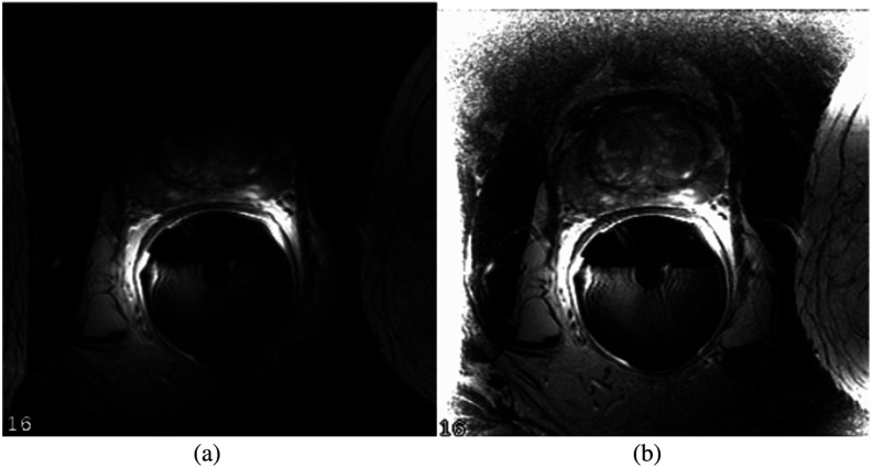
An MR prostate scan can create biased images from different scanning protocols. The artifacts sometimes appear on the image as black regions, which hide certain parts of the prostate. To improve the quality of the images from the acquisition, we first apply N4 correction to remove bias field distortion on the image. The N4ITK16 algorithm is used to correct nonuniformity within each given MR prostate image. Figure 2 demonstrates the image quality before and after applying N4 correction.
Fig. 2.
N4 correction. PROMISE-12 training case 12: (a) before and (b) after.
2.2.3. Isotropic upsampling
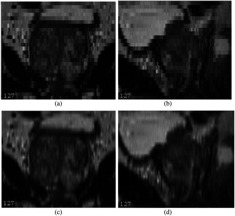
For the given NIH data, the axial MR image resolution is . The plane of the axial image presents the finer detail of prostate with high resolution. However, the slice thickness is 3 mm, and the coronal and sagittal view planes from an axial image only represent the prostate at a coarse level, which is prone to blurring and staircasing artifacts. Figures 3(a) and 3(b) show the coronal and sagittal views before upsampling. To get a reasonable spatial context information from the 3-mm low-resolution view, we isotropically upsample the image to resolution. We use MIPAV17 trilinear interpolation to upsample the axial image. Figures 3(c) and 3(d) illustrate the coronal and sagittal views after upsampling.
Fig. 3.
Axial image isotropic upsampling: (a) coronal before, (b) sagittal before, (c) coronal after, and (d) sagittal after.
2.2.4. Reorientation
After upsampling the axial image into isotropic resolution, we interpolated and reoriented the axial image with corresponding binary VOI masks into coronal and sagittal images. Figure 3 shows the effect after converting from the axial image. By taking advantage of the spatial contextual information from three orthogonal views, we build up the 2-D approach to segment the prostate and central gland.
2.2.5. Coherence enhanced diffusion
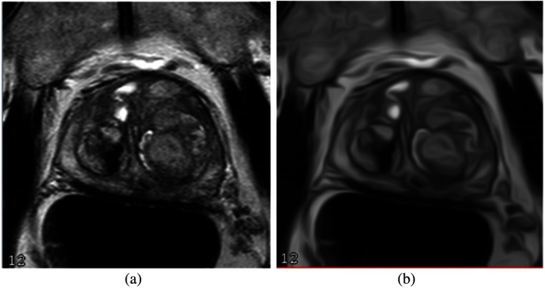
For the MRI alone, the noise and low-contrast regions contribute to the major artifacts. As a consequence, some edge boundaries might be missing or blended with the surrounding tissues. We apply a CED filter based on Ref. 18 to obtain the boundary-enhanced feature image. The CED filters enhance the gray-level edge boundaries, which can remove noise to improve HNN performance. The CED image operation is shown in Fig. 4.
Fig. 4.
CED filter: MR image and (b) CED image.
2.2.6. Intensity normalization
To overcome the intensity variability of MR prostate images, we apply the interquartile range (IQR) method to scale the image intensity range between 0 and 1000, then rescale between [0, 255] to standard PNG file format. The IQR is the difference between the first and third quartiles, i.e., 25% and 75%. The IQR scaling is calculated as
| (1) |
where is the intensity set of the whole 3-D image after sorting and is the unscaled voxel intensity. Figure 5 shows the intensity normalization step.
Fig. 5.
Median and IQR intensity normalization: (a) before and (b) after.
After the preprocessing step, axial, coronal, and sagittal view images and corresponding binary masks are converted into 2-D slices with PNG file format. The newly generated MR image and CED image slice pairs with corresponding ground truth are used to train and test the deep learning model.
2.3. Proposed Deep Learning Architecture
2.3.1. Schema overview
The overall proposed processing pipeline is shown in Fig. 6. From the given low-resolution axial images, we first perform isotropic upsampling followed by reorientation to generate high-resolution orthogonal multiplanar images (axial, coronal, and sagittal). Each orientation is trained and tested with holistically nested network (HNN) or HNNsc models. With the deep learning model predicted VOIs, we utilize 3-D surface reconstruction and mesh optimization as postprocessing to create high-density prostate or central gland surfaces. The final step is to convert the highly dense 3-D surface back into original image low-resolution binary masks for comparison.
Fig. 6.
Proposed segmentation pipeline.
2.3.2. Holistically nested networks architecture
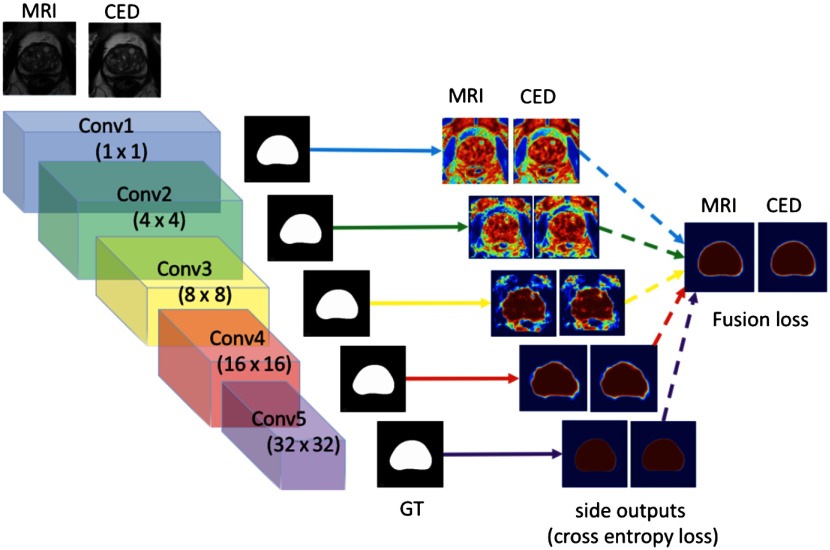
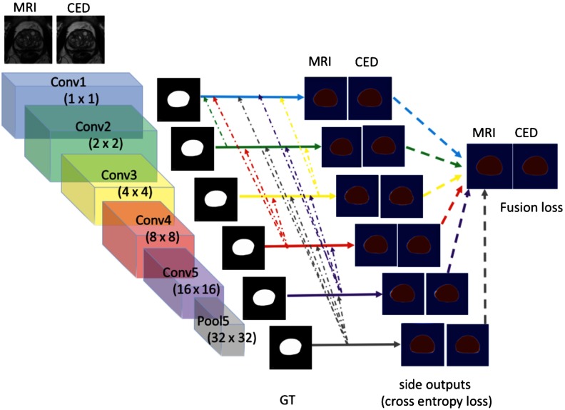
HNN was first proposed by Xie and Tu,19 as a general edge boundary detection method on natural images. Roth et al.20 adapted the HNN architecture for segmenting the interior of organs on medical images, especially for the pancreas segmentation. In previous work,13 we developed an enhanced version of the HNN model.19 The HNN architecture learns the rich hierarchical feature representation and contexts from a general raw pixel-in and label-out mapping function to tackle semantic segmentation tasks in the medical image domain. HNN computes the image-to-image and pixel-to-pixel prediction maps from raw input image to its annotated binary mask, building multiscale and multilevel fully CNNs with deep supervision. The HNN (Fig. 7) consist of five stages. Each stage is scaled with corresponding convolution filters and one additional convolutional layer as side output. Each side output produces a probability map at a single-scale level, and one added fusion layer computes the average of side outputs and generates the final probability map. The entire network is trained with multiple error propagation paths (Fig. 7 side outputs and fusion lines). The HNN model has two folds: (1) holistically training and predicting on the image end-to-end, learning the weight and bias via the per-pixel-based loss function, and (2) leveraging the multiscale and multilevel deep convolutional neural networks to capture the complexity of prostate appearances in MR images.
Fig. 7.
The proposed HNN architecture for MR prostate segmentation.
Experimentally, we found that training and testing the HNN with the MR image data alone occasionally produced unexpected irregular shapes and smaller scattered regions, primarily due to low-edge signals in the MR images. To minimize these problems and to increase the stability of the HNN, we proposed an enhanced HNN model13 that can handle multifeature image pairs. Each MRI and CED image set was paired with the corresponding ground-truth binary mask. Each image pair was a standalone basic unit and together these pairs constitute the training set. The HNN architecture holistically learns the deep representation from both MRI and CED images and builds the internal convolution neural networks between the two image features and corresponding ground truth image maps. The HNN produces per-pixel prostate prediction map pairs (MRI and CED) from each side output layer simultaneously with the ground truth binary mask acting as the deep supervision. The proposed model lets the HNN architecture naturally learn appropriate weights and biases across different features in the training phase.
2.3.3. Holistically nested networks with short connection
Inspired by the recent work of Hou et al.,21 we apply the HNNsc (Fig. 8) model to try to make marginal improvement for segmentation. The intuition of the HNNsc architecture is that the shallower layers side output in the HNN focus on low-level features (finer details, i.e., conv1 side output in Fig. 8) and miss the global context information (coarse-level guidance, i.e., conv5 side output in Fig. 8). The deeper layers side output can find the location or global view of ROI but lose the finer details such as edge boundary. To overcome the drawback, the HNNsc architecture builds the short connections from the deeper layers side output back to the shallower layers side output in order to extract the most visually distinctive object.
Fig. 8.
The proposed HNN short connections architecture for MR central gland segmentation.
To formulate the HNNsc architecture, the side connection of the ’th side output is
| (2) |
where is the short connection weight that back propagates from deeper layers side output to each shallower layer’s side output . The side output function is expressed as
| (3) |
and the fusion loss is
| (4) |
where is the cross-entropy loss, is the fusion weight function, and is the ground truth label. The overall HNNsc loss function is
| (5) |
The HNNsc architecture combines the ROI region lookup and detail refinement steps into the original HNN architecture. The locating step finds the most visually distinguishable ROI region in the deep layers via forward propagation. The details refinement utilizes the top-down approach to build short connections from deep side outputs back to all previous shallower side outputs. Thus the deeper side output guides the shallower layers to more accurately predict the ROI region. Simultaneously, the shallower layers can refine the results from deep side outputs to obtain more dense and accurate prediction maps.
2.4. Postprocessing
Both HNN and HNNsc architectures can produce reasonable segmentation results along each orthogonal view. However, the generated binary prostate or central gland masks occasionally contain erroneous segmentation. Some cases have obvious offset from ground truth masks, even at the central prostate slices, as shown in Fig. 9.
Fig. 9.
Erroneous contours predicted from HNN model: (a) axial segmentation, (b) coronal segmentation, and (c) sagittal segmentation. Green contours are the ground truth and red contours are the HNNsc predicted results. HNNsc generated contours have obvious offset from the ground truth contours.
This is due to a problem of the training data not representing these challenging cases from the test data or overfitting and generalization issues, which model the training data too well and fail to generalize to new unseen data. The HNN and HNNsc architectures cannot guarantee that the end-to-end prediction generates the perfect segmentation solution. No matter which deep learning architecture is applied, U-Net, DenseNet, or the proposed HNN architecture, the unexpected irregular shapes of prostate exist randomly in the MR-based segmentation tasks. In 2-D stand-alone approach for an axial image, most erroneous contours appear at apex and base due to incorrect prediction. Those errors could be reduced from the triplanar spatial context. This is the key reason that the 2-D orthogonal approach is proposed. Finally, we apply 3-D surface reconstruction to build the prostate and central gland 3-D surfaces from the cloud point sets. We further refine the 3-D surface with mesh optimization.
2.4.1. Bounding-box based errors reduction
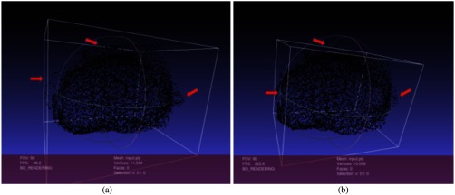
When we merge the axial, sagittal, and coronal VOIs from the deep learning generated results, the aforementioned irregular shapes can have obvious outward points from the base. The simplest and most effective way is to build a minimum bounding box to remove the outward points. We search each axial, coronal, and sagittal VOI contour to find min and max , , coordinates for each orthogonal VOI, then using the minimum bounding box to remove the outside points. Figure 10 illustrates the effect before and after applying the min bounding box.
Fig. 10.
Min bounding box to remove noise contour points: (a) the HNN predicted points after merging the three VOIs. The deep learning model occasionally produces unexpected shapes and (b) min bounding box removes outward points and moves the bounding box planes close to the majority prostate cloud points.
2.4.2. 3-D surface reconstruction
The given images are all in the axial orientation. After isotropic upsampling and reorientation steps, the axial image still keeps the high resolution in the plane. The generated coronal and sagittal views are still coarse but contain more contextual information than the low-resolution (3 mm) images. Along each direction, each orientation image has a large number of slices after isotropic upsampling. While the merged cloud points are much denser, they contain a lot of noisy points internally (due to HNN segmentation error) and externally around the 3-D surface. The ball-pivoting22 and Poisson surface reconstruction algorithms23 are used to generate a smoothed high-resolution 3-D surface out of the noisy points. Figure 11 illustrates the 3-D surface created from ball-pivoting and Poisson algorithms.
Fig. 11.
Central gland 3-D surface reconstruction: (a) ball-pivoting output. (b) Poisson output.
2.4.3. 3-D mesh optimization
Some 3-D surfaces after ball pivoting and Poisson reconstruction still look bumpy due to the predefined ball radius and point cloud complexity. To approximate a smooth surface, we apply the VTK Laplacian smoothing algorithm.24 The effect is to reduce the high-surface curvature and flatten the bumpier or coarser meshes. Those small curvature or bumpier patch artifacts from the 3-D surface reconstruction procedure can be further reduced. The 3-D surface quality depends on the parameters setting of the ball pivoting and the Poisson algorithm, i.e., ball radius, Poisson octree traversing depths, etc. Occasionally, the BPA and PA reconstructed 3-D surface can still be coarse. Thus 3-D surface smoothing is important in creating high-quality surface and in approximating the real prostate or central gland shapes. Overall, the surface reconstruction and mesh optimization together warrant a smooth 3-D surface being constructed from the noisy cloud points.
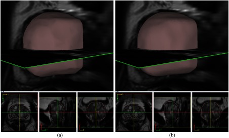
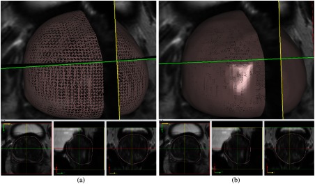
After the 3-D surface is created, we need to convert the 3-D prostate surface back into 2-D prostate binary masks for evaluation. We compute the 3-D surface and 2-D slices intersection points from the 3-D mesh subdivision in image space. The nonuniform subdivision25 algorithm is used to subdivide the 3-D surface multiple times (i.e., 50). We subdivide the 3-D surface into much denser triangles, then compute the closest points to the specific slice number. We use a polar coordinate system to extract the 2-D VOI contours from the interpolated intersection points. The method is simple and effective. It also generates the 2-D binary masks with less information loss. Conservatively, we apply the 3-D morphology identity function to the binary mask image to further remove scattered noisy points on the binary mask image. Finally, the 2-D binary mask is transformed back to the original image space (low resolution in axial image) for comparison. Figure 12 shows the subdivision effect.
Fig. 12.
3-D prostate surface subdivision: (a) before subdivision and (b) after subdivision.
3. Experiments
3.1. Training and Testing
The NIH dataset includes 145 axial MR images with dimensions of and resolutions of . Both whole prostate and central gland VOIs are given as the ground truth. Fivefold cross validation is used for the experiments. Two experiments (HNN and HNNsc) are conducted for each fold to evaluate the segmentation performance. For each orientation (axial, coronal, and sagittal), we train a 2-D-based standalone model; three models formulate the 2-D orthogonal approach. After preprocessing, around 45,000 2-D slice pairs [MRI slice with ground truth (GT) mask and CED slice with GT mask] are mixed (pair wise) together to train one stand-alone HNN or HNNsc model. During the testing phase, the tested images run against each trained model to generate the VOIs for each orientation. Surface reconstruction and mesh optimization are used to create a highly dense 3-D surface from the HNN- or HNNsc-predicted VOIs. Then the 3-D surface is converted back to binary mask images for comparison. The whole prostate and central gland segmentations are conducted as separate experiments.
The PROMISE-12 dataset has 50 prostate MR images for training and 30 images for testing. We perform experiments with HNNsc model for prostate segmentation only. The training and testing follow the same procedure as described above. Testing is evaluated by the PROMISE-12 organizers.
3.2. Implementation
All the preprocessing, postprocessing, 3-D surface reconstruction, mesh optimization, and 3-D visualization are all implemented with the MIPAV application. HNN19 and HNNsc21 are implemented using the Caffe library (C++ and Python). The HNN and HNNsc hyperparameter settings are the same: batch size (1), learning rate (), momentum (0.9), weight decay (0.0002), number of training iterations (30,000), and step size (10,000). The fusion layer side output generates a [0, 1] probability map, which is scaled to [0, 255] intensity range. During postprocessing, we convert the probability map into a binary mask using threshold at to extract the whole prostate and the central gland. The threshold level has been found as optimal on both the NIH dataset and Promise 12 dataset. We then generate final VOI contours from the binary mask.
3.3. Evaluation
The 3-D prostate or central gland surfaces are converted back to the original image space (low resolution) binary masks to compare with the ground truth. The evaluation metrics for NIH data include Dice similarity coefficient (DSC), Jaccard (IoU), Hausdoff distance (HD, mm), and average minimum surface-to-surface distance (AD, mm). EvaluateSegmentation26 is utilized to evaluate segmentation performance. No trimming is applied to any ending contours, such as a 5% or 95% trimming interval to remove outliers for distance-based measure and DSC measure. Incorrect prediction (i.e., under or over segmentation slices at apex and base) are counted into the final measurement results. Statistical significance of differences in performance measure between the HNN models is computed using the Wilcoxon signed-rank test for the value. Tables 1 and 2 demonstrate the whole prostate and central gland segmentation accuracy performance by comparing the HNN and HNNsc models.
Table 1.
Whole prostate segmentation. The prostate segmentation results of two proposed methods, HNN, HNNsc, four metrics DSC (%), Jaccard index (%), HD (mm), and AD (mm). The statistical significance when comparing between the two methods is Wilcoxon signed-rank test with .
| DSC (%) | Jaccard IoU (%) | HD (mm) | AD (mm) | |||||
|---|---|---|---|---|---|---|---|---|
| HNN | HNNsc | HNN | HNNsc | HNN | HNNsc | HNN | HNNsc | |
| Mean | 90.01 | 92.35 | 81.97 | 85.92 | 11.95 | 8.49 | 0.14 | 0.11 |
| Std | 2.99 | 3.00 | 4.82 | 5.01 | 8.73 | 2.99 | 0.07 | 0.06 |
| Median | 90.45 | 92.89 | 82.56 | 86.73 | 9.64 | 8.06 | 0.12 | 0.09 |
| Min | 78.91 | 81.30 | 65.17 | 68.50 | 3.00 | 3.16 | 0.05 | 0.03 |
| Max | 95.21 | 97.39 | 90.86 | 94.91 | 63.01 | 20.22 | 0.48 | 0.39 |
Note: Bold values indicate the best results.
Table 2.
Central gland segmentation. The central gland segmentation results of two proposed methods, HNN, HNNsc, four metrics DSC (%), Jaccard index (%), HD (mm), and AD (mm). The statistical significance when comparing between the two methods is computed by Wilcoxon signed-rank test with .
| DCS (%) | Jaccard IoU (%) | HD (mm) | AD (mm) | |||||
|---|---|---|---|---|---|---|---|---|
| HNN | HNNsc | HNN | HNNsc | HNN | HNNsc | HNN | HNNsc | |
| Mean | 88.03 | 90.06 | 78.99 | 83.06 | 9.01 | 9.35 | 0.20 | 0.16 |
| Std | 5.62 | 4.71 | 7.68 | 7.35 | 5.29 | 4.56 | 0.24 | 0.14 |
| Median | 89.04 | 91.60 | 80.25 | 84.51 | 7.68 | 8.36 | 0.15 | 0.11 |
| Min | 41.34 | 69.69 | 26.05 | 53.48 | 2.82 | 3.6 | 0.05 | 0.04 |
| Max | 95.25 | 96.88 | 90.94 | 93.96 | 44.5 | 29.7 | 2.81 | 0.77 |
Note: Bold values indicate the best results.
We observe that the HNNsc model improves the mean DSC by 2% with (i.e., prostate: 90.01% to 92.35%; central gland: 88.03% to 90.06%), the mean IoU by 4% with (i.e., prostate: 81.97% to 85.93%; central gland: 78.99% to 83.06%). In current MR prostate segmentation literature, 2% performance improvement is significant, especially for DSC results close to or better than 90%.
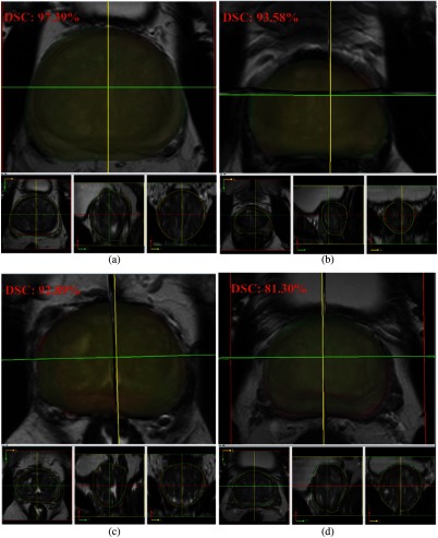
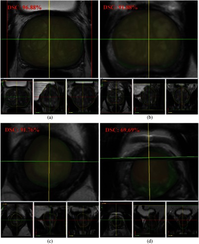
Visual comparison of the HNNsc segmented whole prostate and central gland results are shown in Figs. 13 and 14. The 3-D surfaces are on the top, followed by VOI contours at the bottom. In general, the HNNsc model illustrates promising segmentation results from the best and normal cases. In worst case scenario, the whole prostate segmentation [Fig. 13(d)] has a certain offset from the ground truth. Perceptually, the HNNsc result is acceptable due to the anatomic structure. The central gland segmentation [Fig. 14(d)] reflects an incorrect prediction case from HNNsc prediction (coronal, sagittal, and 3-D views), which is under-segmented. Overall, the mean DSC and HD values of HNN and HNNsc demonstrate the promise and robustness of the segmentation pipeline.
Fig. 13.
HNNsc segmentation result of whole prostate: (a) best result, (b) and (c) average results, and (d) worst result.
Fig. 14.
HNNsc segmentation result of central gland: (a) best case, (b) and (c) average cases, and (d) worst case.
Direct quantitative comparison with other methods from the literature is not possible due to differences in image datasets and number of images used in the experiments during training and testing. Table 3 lists DSC and HD values to roughly compare the latest literature results. The proposed HNNsc model has a mean DSC of 92.35% on NIH dataset (145 images) under the fivefold cross-validation scheme. The evaluation scheme does not trim any erroneous contours at apex and base (i.e., trim lower 5% and higher 95%). To our best knowledge, the proposed 2-D orthogonal HNNsc segmentation model achieves comparable results to the-state-of-the-art literature results.
Table 3.
Comparison with latest literature results of the whole prostate segmentation.
| Methods | (%) | HD (mm) | Images | Eval method | Trim-95% | Year |
|---|---|---|---|---|---|---|
| Zhu10 UR-Net | 93.61 | 80 | Train:76, test:4 | Yes | 2018 | |
| He27 BT + CNN-ASM | Promise-12 | Train:50, test:30 | Yes | 2017 | ||
| Jecevicius28 AAM | 93 | 4.12 | Promise-12 | 50-fold, leave-one-out | Yes | 2017 |
| Meyer9 3D-CNN | 92.10 | Prostate- | Train: 25, test: 15 | Yes | 2018 | |
| Yu7 U + Res net | 89.43 | 5.54 | Promise-12 | Train: 50, test: 30 | Yes | 2017 |
| Jia11 ensemble | Promise-12 | Fourfold cross validation | Yes | 2018 | ||
| Our HNNsc | 145 (NIH) | Fivefold cross validation | No | 2018 | ||
| Our HNNsc | Promise-12 | Train: 50, test: 30 | Yes | 2018 |
3.4. Ablation Study
One ablation study we conducted applies the proposed HNNsc method to the PROMISE-12 challenge dataset. We train the 50 training images thoroughly without fine-tuning the training set images for better performance. The quantitative results for the 30 testing cases are shown in Table 4. We compare our results with a few methods from the leaderboard. We come close to the performance of the top ranked teams (September 2018, as of written). Future work will aim to improve apex and base performance.
Table 4.
Comparison with a few PROMISE-12 challenge leaderboard methods. Three metrics DSC (%), (HD, mm), and average boundary distance (ABD, mm).
| Ours | Phlilips DL_MBS29 | CUMED | Emory | Individual | ||
|---|---|---|---|---|---|---|
| Method | HNNsc | CNN | 3-D V-net | Superpixel | DenseFCN | |
| Whole | ||||||
| DSC (%) | Apex | |||||
| Base | ||||||
| HD (mm) | Whole | |||||
| ABD (mm) | Whole |
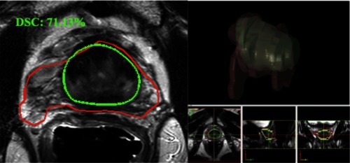
One other ablation study compares the proposed result to one previous work. We proposed the enhanced HNN MRI + CED segmentation model13 for axial image alone. In the worst case scenario, we encountered noticeable volume difference and high HD errors, which are primarily contributed from the erroneous contours at the apex and base. Figure 15 illustrates one worse case. HNN model generates unpredictable results occasionally. HNN prediction errors cannot be eliminated with axial context alone. With the proposed 2-D orthogonal context, the HNN prediction errors can be effectively reduced via low-resolution coronal and sagittal views.
Fig. 15.
One worst case segmentation result from the enhanced HNN model on axial image alone. Image from Ref. 13. Ground truth (green) and segmentation (red). The 3-D surface is constructed from a marching cube algorithm.
In our previous work,13 we utilized 250 datasets from NIH, and all axial images are acquired from ERC insertion. In this proposed work, we utilize mixed data from a NIH multi-institutional study and a few datasets from the ProstateX challenge, a total of 145 datasets. The ERC context is mixed. The proposed axial image segmentation pipeline alone (Fig. 6) follows exactly the model setup in Ref. 13. We compare axial image segmentation alone with the proposed 2-D orthogonal segmentation model using 145 datasets as an approximation to compare with the previous work.13 Table 5 demonstrates the mean value of the four metrics. The HNN 2-D orthogonal model outperforms HNN axial alone by (Dice score) with . The HNNsc 2-D orthogonal model outperforms HNN axial alone by 3% (Dice score) with , which is significant. The HNNsc mean HD error is reduced by 4 mm from the HNN axial alone.
Table 5.
Approximate comparison with our previous work,13 using the NIH 145 dataset to compare axial image alone segmentation results with proposed 2-D orthogonal segmentation results. Four metrics: DSC (%), Jaccard index IOU (%), HD (mm), and AD (mm).
| Mean | HNN_axial | HNN | HNNsc |
|---|---|---|---|
| (mm) | |||
| (mm) |
One other interesting study investigates the impact of HNN versus 2-D U-Net. We segment the prostate (orthogonal context, fivefold cross validation) with the NIH 145 dataset by replacing HNN or HNNsc pipeline part completely with 2-D U-Net architecture in the proposed paradigm (Fig. 6). We ensure that the remaining pipeline is the same, such as preprocessing, MRI and CED pairs, orthogonal segmentation, postprocessing with 3-D surface reconstruction, and optimization. For simplicity, we slightly change the 2-D U-Net implementation30,31 to run the experiment with the closest HNN hyperparameter settings: image size (), batch_size (8), epochs (100), learning rate (), momentum (0.9), optimization (SGD, stochastic gradient decent), and decay rate (). Table 6 illustrates the segmentation performance. Both HNN and HNNsc outperform the 2-D U-Net in all four measures, showing that HNN-based architectures provide an advantage over 2-D U-Net. HNN- and HNNsc-based architectures have noticeably improved the performance by 16% and 18%, respectively, () on the average DSC as compared with 2-D U-Net.
Table 6.
Replacing HNN part pipeline with 2-D U-Net and comparing prostate segmentation results between 2-D U-Net and HNN on axial image using the NIH 145 dataset. Four metrics: DSC (%), Jaccard index IOU (%), HD (mm), and AD (mm).
| Mean | 2-D U-Net | HNN | HNNsc |
|---|---|---|---|
| (mm) | |||
| (mm) |
4. Discussion and Conclusion
In this work, we propose a 2-D orthogonal HNNsc deep learning framework to accurately segment the prostate and central gland volumes in MR images. The framework utilizes the axial, sagittal, and coronal images to reconstruct high-density 3-D prostate and central gland surfaces from the low-resolution axial images. Traditional 2-D schemes with axial image alone suffer from prediction errors. Even with the latest proposed deep learning methods, irregular shapes and scattered small regions could appear in the central part, apex, and base part of the predicted probability maps. To overcome the problems, the proposed 3-D surface reconstruction and optimization step can approximate the real prostate and central gland 3-D shapes from deep learning predicted probability maps and effectively reduce the noise regions.
Several latest literature works7–9 integrate the deep learning model into the MR prostate segmentation and show promising results. They all stem from the 3-D-convolution filter with U-Net architectures, which are all end-to-end prediction systems. Brosch and Saalbach32 mentioned that 3-D U-Net requires a large amount of GPU memory in the training step and performs poorly on the training images. A few drawbacks cause a substantial bottleneck in the 3-D-Conv U-Net approach: (1) image size and resolution limitation. Small 3-D blocks extraction (overlapped sliding window, random sampling, and data augmentation) from the large image is time-consuming and is prone to over-fitting issues during the deep learning training phase. Since only a small fraction of 3-D volume blocks represent the real prostate boundary, remaining blocks from internal and external regions will be labeled as negative 3-D patches. As we mentioned in Sec. 1, all the three proposed works apply 3-D-Conv U-Net to either small images or low-resolution images. (2) Limited GPU memory can prevent the architecture from scalability issues. For example, training 3-D U-Net convolution on a general purpose 5 GB texture memory card (Nvidia k20 card) for large datasets is infeasible and prohibitively expensive. In contrast, we propose the 2-D orthogonal approach. We apply HNN or HNNsc model to each upsampled axial, coronal, and sagittal image as a standalone model. Then spatially aggregate the multiple orthogonal view VOIs to reconstruct 3-D surfaces. The substantial advantages are: (1) 2-D HNN or HNNsc is computationally efficient. This 2-D MRI and CED slice pairs mechanism can fit into a large number of images with high resolution and large image size in both training and testing phases. It also scales well on a general purpose graphics card. (2) The spatial aggregation of orthogonal views could be an efficient way to diminish the curse of dimensionality from their 3-D counterparts. Volumetrically, the proposed framework can still get reasonable spatial context. (3) We apply the whole framework to the low-resolution axial image alone. One big concern is that the low-resolution coronal view and sagittal view might impose segmentation ambiguities from the deep learning model. We utilize isotropic upsampling to generate finer axial, coronal, and sagittal viewing images and apply a CED filter to enhance the edge boundary. We find experimentally that the 2-D orthogonal approach obtains reliable segmentation results. The experiments show that using the low-resolution coronal and sagittal views is a viable approach to fine-tuning multiple aggregations for MR prostate segmentation tasks.
In the previous work,12 we applied HNN and 3-D reconstruction models to MR images alone. The orthogonal viewing images (high-resolution axial, sagittal, and coronal) were given from an MR scanner with a specific scanning protocol. Recent work13 applied the HNN model with MRI and CED pairs to axial image alone. This system is end-to-end prediction without 3-D surface reconstruction involved. We run into the irregular shapes and scattering noise issues at the prostate central part, apex, and base, which is mainly caused by instability of the HNN deep learning model. In this work, we are only given low-resolution axial images with mixed ERC coil context. The proposed framework has a few advantages over the previous works: (1) it integrates the upsampling step to an axial image to get finer context information from orthogonal views. (2) 3-D surface reconstruction and optimization effectively reduce noise from deep learning prediction. (3) The HNNsc back-propagates the global context to all previous side output layers to increase robustness of the deep learning prediction. Experimentally, the HNNsc deep learning model with short connections elevates the DSC segmentation performance by 2% from the HNN model.
Meyer et al.9 proposed a similar approach from multiplanar volumes. They were given high-resolution axial, sagittal, and coronal images from the MR scanners. They co-register the three volumes to make context alignment. Then they apply multistream 3-D U-Net convolution architecture to all three volumes with marching cubes as the postprocessing step to generate a smooth 3-D prostate surface. To distinguish from this work,9 we take a standalone HNN or HNNsc model to each orthogonal view image, which is obtained from upsampling and re-interpolation of the low-resolution axial images. The reason is obvious. There should not be any correlation across orthogonal views in a 2-D context, i.e., the correlation between 2-D coronal and sagittal slices. We could merge all three views to train one deep learning model to adapt the multistream paradigm. Conservatively, we consider this multistream mechanism for 2-D context could be error prone. The separate training model can avoid ambiguities among the orthogonal context in 2-D. Even with the proposed 2-D HNNsc model, direct end-to-end prediction cannot avoid noise regions in all three orthogonal views. The proposed postprocessing step plays a crucial role to effectively reduce noise. The ball radius of the ball-pivoting algorithm avoids obvious convex and concave components from the cloud points and not all points need to be visited via ball pivoting. The Poisson algorithm can further remove holes on the 3-D surface. Thus the postprocessing step can refine the high-density 3-D surfaces from the deep learning predicted noisy cloud point set. To the best of our knowledge, the marching cubes algorithm visits every point in the cloud point set, and it cannot skip the convex or concave shapes on the 3-D surface. Also the multistream 3-D U-Net convolution model cannot guarantee the predicted point cloud set is noise free. Those scattered noise regions cannot be effectively removed or reduced using the marching cubes surface reconstruction mechanism. The proposed 3-D postprocessing step (min bounding box reduction → Ball pivoting and Poisson reconstruction → mesh optimization) only takes around 20 to 30 s to create one 3-D surface from the cloud point set on general CPU (i.e., Intel i7) during a low computational cost testing phase.
In addition to 3-D U-Net-based image segmentation, one other interesting perspective is incorporating 3-D mesh-based training with the convolution neural networks, which is a very challenging task. One ideal state traces the 3-D mesh normal lines with the texture-based convolution operation to find the optimal convergence point. The nature of 3-D convolution makes controlling the topology path of mesh optimization hard during the convolution since the CNN neural connections between convolution layers distort the topology path for the 3-D mesh traversal. Brosch et al.29 presented a typical work in this direction. The method initializes a 3-D mesh using model-based segmentation;33 then a neural network-based boundary detection architecture achieves the 3-D mesh optimization with the CNN convolution. Small 3-D subvolumes sampled along the normal line of the center point of a triangle are the basic convolution units, which collect the 3-D texture features. The signed distance between the center of the triangle and the correct prostate boundary (the ground truth) is used as the optimization function to build the parametric adaption neural network. Two stages coarse-to-fine boundary detection networks are the primary architecture: a global boundary detector that uses the same parameters to optimize all the triangles to adapt the 3-D mesh close to the right boundary; and a locally adaptive network that adds a triangle-specific weighting layer to the global network to refine the final boundary. During the prediction phase, the proposed method produces a smoothed high-resolution 3-D prostate surface from the last layer of the architecture. Unfortunately, the work is not publicly available, and it is hard to project how the topology path is traversed during the convolution, which needs further clarification. We regard this method as a sound approach to build the bridge between 3-D mesh optimization and 3-D convolution. Our proposed method uses the HNNsc as the primary architecture to find the rough boundary, followed by 3-D mesh optimization and reconstruction to refine. Our approach builds the 3-D geometry after the HNNsc segmentation pipeline. In contrast, Brosch et al.29 performed the 3-D mesh deformed-based training and 3-D reconstruction simultaneously. Brosch et al.29 yielded better performance than us on Promise12 challenge (Table 4). Architecture wise, our method is more straightforward than Brosch et al.29 Our approach can capture orthogonal contextual information and create a smoothed 3-D surface out of the low-resolution images.
To elaborate on the benefits of HNN-based architecture over 2-D U-Net, surprisingly, the experimental results from Table 6 demonstrate the improvement over 2-D U-Net by replacing it with a HNN pipeline. Our observation is that 2-D U-Net requires a huge hyperparameter space to train a model with a large dataset. With our training scenario (50k MRI and CED pairs), 2-D U-Net is relatively unstable as the baseline segmentation model. During the prediction phase, we can see a lot of miss and over segmentations in the central part, apex, and base of the prostate. Scaling up to a large training dataset is the drawback of 2-D U-Net and might require further extensive hyperparameter tuning. In contrast, the HNN-based architecture is smaller and simpler than 2-D U-Net and HNN does not have the scaling issue with the large training dataset. Even the general purpose graphics card (i.e., Nvidia card with 6 GB texture memory) can easily fit into the HNN hyperparameter training space with our training scenario. The 2-D U-Net requires a 10-stage encoding–decoding path, which significantly downgrades the training and prediction efficiency, preventing its use for large-scale segmentation tasks, and increases the uncertainty to create unexpected noise. The HNN architecture simplifies the CNN architecture by eliminating the decoding path of the 2-D U-Net, reducing its size by half. It is a feed-forward neural network capable of producing multiscale outputs in a single path, resulting in minimal resources required in both training and testing. The HNN training and prediction is based on the whole image end-to-end (holistically) using per-pixel labeling cost. HNN incorporates multiscale and multilevel learning of deep image features via auxiliary cost functions at each convolutional layer. It is capable of automatically learning the rich hierarchical feature representations (contexts) that are critical in resolving multiscale spatial segmentation. The stability of the HNN architecture, its ability to capture texture variation across the full image context, and the large training set promote the superior performance of the HNN model.
In conclusion, we present a 2-D orthogonal HNNsc framework to automatically segment the MR prostate and central gland from the axial images alone. The preprocessing step enhances the MR image quality and converts the low-resolution axial image to high-resolution orthogonal view images. The 2-D HNNsc deep learning model exploits multifeatures (MRI + CED pair) to generate reasonable segmentation probability maps. The short connections from deep side output layers back to all shallower side output layers ensure more robust prediction. The HNNsc model improves the segmentation performance from the HNN model by 2% in mean DSC. The postprocessing step refines the 3-D smooth surfaces from the HNNsc generated noisy cloud point set and converts the highly dense 3-D surface back to a low-resolution axial image. Traditional 2-D deep learning segmentation models rarely use the low-resolution coronal and sagittal views due to potential ambiguities imposed from the deep learning model. We isotropically upsample the low-resolution axial image and multiaggregate the orthogonal views as spatial context to enhance the segmentation accuracy. The experimental results verify that the proposed framework is a relatively simple, feasible, and reliable approach for prostate segmentation tasks. In addition, the proposed framework achieves close to state-of-the-art performance as compared with other literature results. In the current literature, we are one of the few works to propose the deep learning model for both MR prostate whole and central gland segmentation, which can substantially aid the prostate cancer detection in a CAD system.
Acknowledgments
This work was supported in part by the Intramural Research Program of the National Institutes of Health, Clinical Center, National Cancer Institutes, and CIT. We thank NVIDIA for Titan X GPU donations to our groups. This research used the high-performance computing capabilities of the NIH Biowulf GPU clusters.
Biography
Biographies of the authors are not available.
Disclosures
Author R. M. S. reports royalties from iCAD, Philips, ScanMed, and PingAn, and research support from PingAn and NVIDIA. No conflicts of interest, financial or otherwise, are declared by the authors.
References
- 1.Klein S., et al. , “Automatic segmentation of the prostate in 3-D MR images by atlas matching using localized mutual information,” Med. Phys. 35(4), 1407–1417 (2008). 10.1118/1.2842076 [DOI] [PubMed] [Google Scholar]
- 2.Yin Y., et al. , “Fully automated prostate segmentation in 3-D MR based on normalized gradient fields cross-correlation initialization and LOGISMOS refinement,” Proc. SPIE 8314, 831406, (2012). 10.1117/12.911758 [DOI] [Google Scholar]
- 3.Ghose S., et al. , “Texture guided active appearance model propagation for prostate segmentation,” Lect. Notes Comput. Sci. 6367, 111–120 (2010). 10.1007/978-3-642-15989-3 [DOI] [Google Scholar]
- 4.Toth R., Madabhushi A., “Multifeature landmark-free active appearance models: application to prostate MRI segmentation,” IEEE Trans. Med. Imaging 31(8), 1638–1650 (2012). 10.1109/TMI.2012.2201498 [DOI] [PubMed] [Google Scholar]
- 5.Habes M., et al. , “Automated prostate segmentation in whole-body MRI scans for epidemiological studies,” Phys. Med. Biol. 58(17), 5899–5915 (2013). 10.1088/0031-9155/58/17/5899 [DOI] [PubMed] [Google Scholar]
- 6.Liao S., et al. , “Representation learning: a unified deep learning framework for automatic prostate MR segmentation,” in 16th Int. Conf. Med. Image Comput. Comput. Assist. Interv., Vol. 16, no. pt2, pp. 254–261 (2013). 10.1007/978-3-642-40763-5_32 [DOI] [PMC free article] [PubMed] [Google Scholar]
- 7.Yu L., et al. , “Volumetric ConvNets with mixed residual connections for automated prostate segmentation from 3-D MR images,” in Proc. Thirty-First AAAI Conf. Artif. Intell., pp. 66–72 (2017). [Google Scholar]
- 8.Milletari F., Navab N., Ahmadi S. A., “V-net: fully convolutional neural networks for volumetric medical image segmentation,” in Fourth Int. Conf. 3-D Vision (3DV) (2016). 10.1109/3DV.2016.79 [DOI] [Google Scholar]
- 9.Meyer A., et al. , “Automatic high resolution segmentation of the prostate from multi-planar MRI,” in IEEE 15th Int. Symp. Biomed. Imaging (ISBI) (2018). 10.1109/ISBI.2018.8363549 [DOI] [Google Scholar]
- 10.Zhu Q., et al. , “Exploiting interslice correlation for MRI prostate image segmentation, from recursive neural networks aspect,” Complexity 2018, 4185279 (2018). 10.1155/2018/4185279 [DOI] [Google Scholar]
- 11.Jia H., et al. , “Atlas registration and ensemble deep convolutional neural network-based prostate segmentation using magnetic resonance imaging,” Neurocomputing 275(C), 1358–1369 (2018). 10.1016/j.neucom.2017.09.084 [DOI] [Google Scholar]
- 12.Cheng R., et al. , “Deep learning with orthogonal volumetric HED segmentation and 3-D surface reonstruction model of prostate MRI,” in IEEE 14th Int. Symp. Biomed. Imaging (ISBI), pp. 749–753 (2017). 10.1109/ISBI.2017.7950627 [DOI] [Google Scholar]
- 13.Cheng R., et al. , “Automatic magnetic resonance prostate segmentation by deep learning with holistically nested networks,” J. Med. Imaging 4(4), 041302 (2017). 10.1117/1.JMI.4.4.041302 [DOI] [PMC free article] [PubMed] [Google Scholar]
- 14.Armato S., et al. , “PROSTATEx challenge 2017,” 2017, https://spie.org/x115569.xml?wt.mc_id=rmi17gb.
- 15.Litjens G., et al. , “The PROMISE12 segmentation challenge,” 2012, https://promise12.grand-challenge.org/.
- 16.Tustison N. J., et al. , “N4ITK: improved N3 bias correction,” IEEE Trans. Med. Imaging 29(6), 1310–1320 (2010). 10.1109/TMI.2010.2046908 [DOI] [PMC free article] [PubMed] [Google Scholar]
- 17.McAuliffe M. J., et al. , “Medical image processing, analysis, and visualization in clinical research,” in Proc. 14th IEEE Symp. Comput. -Based Med. Syst. (CBMS), pp. 381–386 (2001). 10.1109/CBMS.2001.941749 [DOI] [Google Scholar]
- 18.Weickert J., “Coherence-enhancing diffusion filtering,” Int. J. Comput. Vision 31(2), 111–127 (1999). 10.1023/A:1008009714131 [DOI] [Google Scholar]
- 19.Xie S., Tu Z., “Holistically-nested edge detection,” in Proc. IEEE Int. Conf. Comput. Vision (ICCV), pp. 1395–1403 (2015). 10.1109/ICCV.2015.164 [DOI] [Google Scholar]
- 20.Roth H. R., et al. , “Spatial aggregation of holistically-nested convolutional neural networks for automated pancreas localization and segmentation,” Med. Image Anal. 45, 94–107 (2018). 10.1016/j.media.2018.01.006 [DOI] [PubMed] [Google Scholar]
- 21.Hou Q., et al. , “Deeply supervised salient object detection with short connections,” IEEE Trans. Pattern Anal. Mach. Intell. 41(4), 815–828 (2019). 10.1109/TPAMI.2018.2815688 [DOI] [PubMed] [Google Scholar]
- 22.Bernardini F., et al. , “The ball-pivoting algorithm for surface reconstruction,” IEEE Trans. Visualization Comput. Graphics 5(4), 349–359 (1999). 10.1109/2945.817351 [DOI] [Google Scholar]
- 23.Kazhdan M., et al. , “Poisson surface reconstruction,” in Eurographics Symp. Geom. Process., pp. 61–70 (2006). [Google Scholar]
- 24.Schroeder W., Martin K., Lorensen B., The Visualization Toolkit, 4th ed, Kitware, New York: (2006). [Google Scholar]
- 25.Lindstrom P., et al. , “Real time, continuous level of detail rendering of height fields,” in ACM SIGGRAPH ‘96 Proc. 23nd Annu. Conf. Comput. Graphics and Interact. Techn., pp. 109–118 (1996). 10.1145/237170.237217 [DOI] [Google Scholar]
- 26.Taha A. A., Hanbury A., “Metrics for evaluating 3-D medical image segmentation: analysis, selection, and tool,” BMC Med. Imaging 15, 29 (2015). 10.1186/s12880-015-0068-x [DOI] [PMC free article] [PubMed] [Google Scholar]
- 27.He B. C., et al. , “Automatic magnetic resonance image prostate segmentation based on adaptive feature learning probability boosting tree initialization and CNN-ASM Refinement,” IEEE Access 6, 2005–2015 (2018). 10.1109/ACCESS.2017.2781278 [DOI] [Google Scholar]
- 28.Jucevicius J., et al. , “Automated 2-D segmentation of prostate in T2-weighted MRI scans,” Int. J. Comput. Commun. Control 12(1), 53–60 (2017). 10.15837/ijccc.2017.1 [DOI] [Google Scholar]
- 29.Brosch T., et al. , “Deep learning-based boundary detection for model-based segmentation with application to MR prostate segmentation,” MICCAI Lect. Notes Comput. Sci. 11073, 515–522 (2018). 10.1007/978-3-030-00937-3 [DOI] [Google Scholar]
- 30.“Lung fields segmentation on CXR images using convolutional neural networks,” https://github.com/imlab-uiip/lung-segmentation-2d (December 2018).
- 31.Ronneberger O., Fischer P., Brox T., “U-Net: convolutional networks for biomedical image segmentation,” Lect. Notes Comput. Sci. 9351, 234–241 (2015). 10.1007/978-3-319-24574-4 [DOI] [Google Scholar]
- 32.Brosch T., Saalbach A., “Foveal fully convolutional nets for multi-organ segmentation,” Proc. SPIE 10574, 105740U (2018). 10.1117/12.2293528 [DOI] [Google Scholar]
- 33.Ecabert O., et al. , “Automatic model-based segmentation of the heart in CT images,” IEEE Trans. Med. Imaging 27(9), 1189–1201 (2008). 10.1109/TMI.2008.918330 [DOI] [PubMed] [Google Scholar]


