Complex Bayesian Modeling Workflows Encoding and Execution Made Easy With a Novel WinBUGS Plugin of the Drug Disease Model Resources Interoperability Framework

Abstract

The Drug Disease Model Resources (DDMoRe) Interoperability Framework (IOF) enables pharmacometric model encoding and execution via Model Description Language (MDL) and R language, through the ddmore package. Through its components and converter plugins, the IOF can execute pharmacometric tasks using different target tools, starting from a single MDL‐encoded model. In this article, we present the WinBUGS plugin and show how its integration in the IOF enables an easy implementation of complex Bayesian workflows. We selected a published diabetes‐linked study as a real‐world example, in which two inter‐related models are used to estimate insulin secretion rate in response to a glucose stimulus from intravenous glucose tolerance test (IVGTT) data. This model was implemented following different approaches to propagate uncertainty, via diverse IOF target tools (NONMEM, WinBUGS, PsN, and Xpose). The developed software supports a plethora of pharmacokinetic/pharmacodynamic (PK/PD) modeling features. It provides solutions to reproducibility and interoperability issues in Bayesian modeling, and facilitates the difficult encoding of complex PK/PD models in WinBUGS.

Study Highlights.

WHAT IS THE CURRENT KNOWLEDGE ON THE TOPIC?

☑ The standard languages and IOF developed within the DDMoRe project facilitate the model encoding and execution tasks using different target tools. Bayesian modeling enables proper prior knowledge integration, uncertainty propagation, and full conditional distribution computation. Complex PK/PD models, such as those described here, are difficult to encode in WinBUGS.

WHAT QUESTION DID THIS STUDY ADDRESS?

☑ We aim to integrate WinBUGS into the DDMoRe IOF, using its interoperable standard languages, and demonstrate its application in an advanced real‐world case study.

WHAT DOES THIS STUDY ADD TO OUR KNOWLEDGE?

☑ The MDL and R can now be easily used to encode and execute complex Bayesian models and workflows in the DDMoRe IOF. We show a variety of reproducible pharmacometric workflows, including Bayesian estimation with propagation of uncertainty and variability through prior specification.

HOW MIGHT THIS CHANGE DRUG DISCOVERY, DEVELOPMENT, AND/OR THERAPEUTICS?

☑ We are lowering the barrier to using WinBUGS and Bayesian methods in pharmacometric workflows.

Bayesian modeling is commonly used to exploit prior knowledge in the parameter estimation process by integrating prior information with experimental data in the posterior distributions of all the parameters of interest.1, 2, 3 This approach also allows the propagation of uncertainty through the different hierarchical levels of a model or among different models and enables direct probabilistic inferences on the posterior distributions.4, 5 Different software tools, such as WinBUGS,6, 7 OpenBUGS,8, 9 Stan,10, 11 JAGS,12, 13 and NONMEM,14, 15 can be used to encode Bayesian models and to carry out parameter estimation via Markov Chain Monte Carlo (MCMC) algorithms.16 WinBUGS enables flexible statistical model specification and relies on additional tools, such as the WinBUGS Development Interface (WBDev)17 with BUGSModelLibrary,18, 19 to cover many features required in pharmacometric modeling, such as custom ordinary differential equations (ODEs), IF‐THEN‐ELSE statements, definition of custom pharmacokinetic (PK) models, and dosing schedules, which are not directly available in the BUGS language.8, 20 The described add‐ons can be integrated within WinBUGS and enable the encoding of customized functions in Component Pascal language,21 including ODE specification, and support the use of NONMEM‐formatted data items.

Considering the other popular or emerging modeling tools mentioned above, although enabling to run several kind of mathematical models, the efficient implementation of pharmacokinetic/pharmacodynamic (PK/PD) models with ODEs and dosing schedules is limited (or missing) in JAGS, Stan, and OpenBUGS,22 even if Stan is currently in further development, and it seems to be a promising tool. The latest versions of NONMEM, the most widely used software for population analysis traditionally done via maximum likelihood approaches, also enable Bayesian analysis via MCMC methods (Gibbs/Metropolis‐Hastings and Hamiltonian/No U‐Turn Sampling). Despite that NONMEM has unique advantages for Bayesian analysis (e.g., parallel computation enabling within‐chain parallelization), and more flexibility has also been given to users with the last release (version 7.4) in terms of prior distribution choices, WinBUGS is recommended when more than two levels of variability or an expanded choice of prior distributions are desired.20, 22, 23, 24, 25 For these reasons, the WinBUGS suite described above represents a key option for Bayesian modeling in the PK/PD context.25, 26, 27, 28

It is worth noting that the WinBUGS suite enables the encoding of complex models, but a significant encoding effort is required, including model and functions definitions via BUGS and Component Pascal languages. Other packages, such as PKBugs,29, 30 Pharmaco,31 and BUGSModelLibrary,18, 19 have been proposed to facilitate pharmacometric models encoding, but they are limited to a set of predefined compartmental models, and the development of more complex ones still requires significant encoding efforts, as described above.25

The Drug Disease Model Resources (DDMoRe) Interoperability Framework (IOF; see Figure 1)32, 33 is a software infrastructure developed by the DDMoRe consortium34 and now supported by the DDMoRe Foundation,35 aimed to facilitate the exchange and integration of models across different languages or tools. The IOF has two key system‐to‐system target tool‐independent interchange standards: Pharmacometrics Markup Language (PharmML), an XML‐based computer language for model representation,36 and standard output (SO), an XML‐based format for storage of pharmacometric analysis results.37 The IOF can be accessed via a graphical user interface, the Modeling Description Language Integrated Development Environment (MDL‐IDE),32 where the user can encode models in MDL,38 and script workflows in R programming language.39 The MDL is a declarative human‐readable/writeable language, characterized by a modular object‐based structure that is used to represent the information required to describe models.38 The MDL facilitates model definition and, in Bayesian estimation, definition of prior distributions for parameters. Specific R functions, available in the ddmore R package,33 support model definition by composing different MDL objects and enabling the execution of the desired modeling tasks.

Figure 1.

Information flow of the Drug Disease Model Resource (DDMoRe) interoperability framework (IOF). The DDMoRe IOF is an integrated set of converters and connectors for many common programming tools and languages. Together with the IOF, the translation of models to different software tools is provided by the integration of two standard languages: Model Description Language (MDL) and Pharmacometric Markup Language (PharmML). A user‐interface, called MDL‐Integrated Development Environment (IDE), allows the user to create and edit files containing MDL code. Alternatively, the user can retrieve and use PharmML and MDL model codes of a variety of state‐of‐the‐art models in key therapeutic areas freely and publicly available in the DDMoRe Model Repository. Once the MDL model code is available, the user can run a specific task (estimation/simulation) in one of the programming tools integrated in the IOF (e.g., WinBUGS) via R code, also specifying the settings that will be passed on to the target tool (variables to be monitored, number of chains, number of updates in the Markov Chain, etc.). Then, three automatic translations are performed in the background: (1) MDL to PharmML model translation; (2) NONMEM‐formatted to BUGS data file translation; and (3) PharmML to WinBUGS model translation, which generates all the necessary model files, including BUGS and Component Pascal files. Then, a connector runs the execution, retrieves the BUGS output (in the form of CODA files), which is then automatically converted into the Standard Output (SO) format by a BUGS to SO output converter. Finally, the connector retrieves the SO file, which becomes available for the user to perform graphical convergence diagnostics and posterior inference.

A set of converters and connectors, described in Figure 1, perform the MDL‐to‐PharmML and the PharmML‐to‐target tool automatic translation, and the execution of a desired task, respectively. Finally, results are provided back to users via SO.

The standardized nature of languages, functions, and outputs in the IOF can significantly alleviate the burden of model/dataset encoding or recoding in different target languages for allowing the exploitation of the different features made available from the different software tools.36 It can support the reproducibility of results and the interoperability among modeling tools, which are long‐standing problems in pharmacometrics, to eventually streamline complex workflows.36, 40, 41

In this work, we aim to present a novel WinBUGS plugin for the IOF and demonstrate its usefulness, power, and flexibility in the programming and execution of a previously published diabetes‐linked Bayesian modeling workflow used as showcase. The developed software framework will provide a solution to interoperability issues in Bayesian modeling and to the currently difficult encoding of complex PK/PD models in WinBUGS. The IOF now supports a wide range of tools for estimation (Monolix, NONMEM, and WinBUGS), diagnostics (PsN and Xpose), simulation (Simulx and SimCyp), and optimization (PopED and PFIM).33

METHODS

Software

The main software modules developed in this work are represented in Figure 1 (with red boxes), and a detailed description of each of them is reported in Supplementary Methods. The version of IOF, including the WinBUGS plugin (version 2.0), used in this article, is freely available at http://aimed11.unipv.it/DDMoReIOF+WinBUGSplugin2.0/, whereas a previous version of the plugin (version 1.0) is integrated into the official IOF public release.33

Implemented example workflow overview

A complex workflow, involving two diabetes‐related published models, has been executed within the IOF and is here proposed as an advanced real‐world case study.

In the diabetic research area, it is of crucial importance to assess the insulin response to a glucose stimulus to understand the β‐cell function in pathological states.42, 43 The intravenous glucose tolerance test (IVGTT) is one of the simplest experiments to do that. To assess insulin response from IVGTT data, the insulin minimal model (MM) is widely used,42, 43, 44 but it requires the knowledge of the individual C‐peptide (CP) kinetics, which is described in the literature by a linear two‐compartment model.45 This model assumes that CP is secreted into the central compartment (compartment 1) from which it is eliminated or it is distributed into the peripheral one (compartment 2). Therefore, CP kinetics is fully characterized by four parameters: k₀₁, k₂₁, k₁₂, and V, where k_ij is the transfer rate from compartment j to i, and V is the central compartment volume. The four parameters in a given individual can be estimated from the knowledge of age, sex, body surface area (BSA), and health condition (normal, obese, or diabetic), using a linear regression model and nonlinear algebraic relationships46, 47 (see below).

All these steps have been implemented in this article following three approaches based on different ways to propagate uncertainty (see Figure 2). The main steps, which are illustrated in detail in Figure 2, include: (1) identification of the population regression model from a large dataset of CP kinetic model parameters (described below); (2) estimation of the CP kinetic parameters of a new subject by using the identified population model; and (3) estimation of insulin secretion rate (ISR) and physiological indexes (e.g., β‐cell sensitivity) by identifying the MM, using the CP kinetic parameters obtained above, and CP and glucose plasma concentration data of the new subject, coming from an IVGTT.

Figure 2.

Modeling approaches implemented in this study. The following number of chains, burn‐in iterations, updates, and thin were used. The M4 identification (full‐Bayesian approach): 1 chain, 1,000 burn‐in iteration, 100,000 updates, thin = 10, repeated for three times, each time using the last values of the chain as initial values for all the population parameters, to eventually obtain 300,000 chain samples; insulin minimal model (MM) identification (full‐Bayesian approach): 1 chain, 1,000 burn‐in iterations, 20,000 updates, thin = 1; MM identification (mixed approach): 1 chain, 1,000 burn‐in iterations, 80,000 updates, thin = 5. CP, C‐peptide; ISR, insulin secretion rate; MLE, maximum likelihood estimate.

Approach 1 (the maximum likelihood estimation (MLE) approach; Figure 2 a) aims to obtain point‐estimates of the variables of interest, without propagating parameter uncertainty throughout the steps 1–3. In this case, the point‐estimates of the CP kinetic parameters, obtained at step 2, are used as fixed parameters of the MM at step 3.

Approach 2 (full‐Bayesian approach; Figure 2 b) aims to provide a statistical framework to properly handle the uncertainty and propagate it through all the workflow steps. In this approach, all the model elements (i.e., data, parameters, and errors) are stochastic variables described by probability distributions. Therefore, the joint distribution of the CP kinetic parameters (obtained at step 2) is used as the prior distribution of these parameters in the MM.

Finally, approach 3 (the mixed approach; Figure 2 c) includes the identification of the MM (step 3) via the Bayesian approach, but fixing the CP kinetic parameters to the values obtained from step 2 via approach 1.

The software tools used via IOF to carry out the described tasks are NONMEM version 7.3, PsN version 4.4.8, Xpose version 4.5.3, and WinBUGS version 1.4 (with BlackBox version 1.521 and BUGSModelLibrary version 1.2).

MATHEMATICAL MODELS

A population regression model to estimate CP kinetic parameters

As reported in ref. 47, the four parameters of the compartment model (i.e., k₀₁, k₂₁, k₁₂, and V), can be obtained from the following macro constants: short half‐life (ts), long half‐life (tl), amplitude fraction (F), and volume of distribution (V), using the algebraic equations below:

$$k_{12}=\ln \left(2\right)\left(\frac{F}{tl}+\frac{1-F}{ts}\right),$$

$$k_{01}=\left(\frac{\ln \left(2\right)}{ts}\right)\left(\frac{\ln \left(2\right)}{tl}\right)\left(\frac{1}{k_{12}}\right),$$

$$k_{21}=\left(\frac{\ln \left(2\right)}{ts}\right)+\left(\frac{\ln \left(2\right)}{tl}\right)-k_{12}-k_{01}.$$

The four macro constants, in turn, can be derived in each subject via four linear regression models:

$${\theta }_{t{s}_i}=\left\{\begin{array}{c}{m}_{tsn}\hspace{0.17em}if HSTATU{S}_i is normal,\\ m_{tso}\hspace{0.17em}if HSTATU{S}_i is obese,\\ m_{tsd}\hspace{0.17em}if HSTATU{S}_i is diabetic,\end{array}\right)$$

$${\theta }_{F_i}=\left\{\begin{array}{c}{m}_{Fn}\hspace{0.17em}if HSTATU{S}_i is normal,\\ m_{Fo}\hspace{0.17em}if HSTATU{S}_i is obese,\\ m_{Fd}\hspace{0.17em}if HSTATU{S}_i is diabetic,\end{array}\right)$$

$${\theta }_{V_i}=\left\{\begin{array}{c}{a}_{Vm}+b_{Vm}·BS{A}_i if SE{X}_i is male,\\ a_{Vf}+b_{Vf}·BS{A}_i if SE{X}_i is female,\end{array}\right)$$

$${\theta }_{t{l}_i}=a_{tl}+b_{tl}·AG{E}_i,$$

where AGE is in years and BSA, expressed in m², is calculated as 0.20247 × Height (m)^0.725 × Weight (kg)^0.425. For the sake of simplicity, we will denote the four regression models as:

$${\mathit{\theta }}_i=\mathit{f}\left(\stackrel{\sim }{\mathit{\theta }},{\mathit{U}}_i\right),$$

where ${ \mathit{\theta }}_i=\left[{\theta }_{t{s}_i},{\theta }_{F_i},\hspace{0.17em}{\theta }_{V_i},{\theta }_{t{l}_i}\right]$ is the vector of the predictions of the four regressions for the i‐th individual, ${\mathit{U}}_i=\left[HSTATU{S}_i,\hspace{0.17em}SE{X}_i,\hspace{0.17em}BS{A}_i,\hspace{0.17em}AG{E}_i\right]$ is the vector of individual covariates, and $\stackrel{\sim }{\mathit{\theta }}=\left[m_{tsn},m_{tso},\hspace{0.17em}{m}_{tsd},\hspace{0.17em}{m}_{Fn},\hspace{0.17em}{m}_{Fo},\hspace{0.17em}{m}_{Fd},\hspace{0.17em}{a}_{Vm},\hspace{0.17em}{b}_{Vm},\hspace{0.17em}{a}_{Vf},\hspace{0.17em}{b}_{Vf},\hspace{0.17em}{a}_{tl},\hspace{0.17em}{b}_{tl}\right]$ is the vector of population parameters.

Interindividual variability on model parameters was assumed to be normally distributed. The individual macro constants ${\mathit{\phi }}_i=\left[{ts}_i,\hspace{0.17em}{F}_i,V_i,t{l}_i\right]$ for the i‐th individual are, therefore, calculated as:

$${\mathit{\phi }}_i={\mathit{\theta }}_i+{\mathit{\eta }}_i,$$

where ${\mathit{\eta }}_i=[{\eta }_{t{s}_i},\hspace{0.17em}{\eta }_{F_i},{\eta }_{V_i},{\eta }_{{tl}_i}]$ is the vector of random effects, which accounts for the interindividual variability. Assuming independent random effects with unknown variance, the described model is equivalent to the one proposed by Van Cauter et al.46 This model version will be referred to as M0.

Following ref. 47, when correlations exist between the elements of ${\mathit{\eta }}_i$, while they are independent between different subjects, we have:

$${\mathit{\eta }}_i\sim N\left(0,\mathrm{\Sigma }\right),$$

where $\mathrm{\Sigma }$ is the full (4 × 4) covariance matrix.

To define a Bayesian model,47 priors on $\stackrel{\sim }{\mathit{\theta }}$ and on ${\mathrm{\Sigma }}^{-1}$are specified:

$$\stackrel{\sim }{\mathit{\theta }}\sim \hspace{0.17em}N\left({\stackrel{\sim }{\mathit{\theta }}}_0,{\mathrm{\Sigma }}_0^{-1}\right),$$

$${\mathrm{\Sigma }}^{-1}\sim W\left(\rho ,\mathit{R}\right),$$

where ${\stackrel{\sim }{\mathit{\theta }}}_0,{\mathrm{\Sigma }}_0$, $\rho ,\hspace{0.17em}\mathit{R}$ are fixed prior parameters and W is the Wishart distribution with mean $\rho ·\mathit{R}$. The following values were chosen according to the original publication: ${\stackrel{\sim }{\mathit{\theta }}}_0=\left[5 5 5 1 1 1 30 1 1 1 1 1\right],\hspace{0.17em}{ \mathrm{\Sigma }}_0$ is a diagonal matrix with ${\stackrel{\sim }{\mathit{\theta }}}_0$ square elements on the diagonal, $\rho =10$, and $\mathit{R}={\rho }^{-1}{\left(0.01·diag\left(\left[5 1 30 4\right]\right)\right)}^{-1}$. This Bayesian model version will be referred to as M4.

The MDL code of the described models is freely available for downloading in the DDMoRe Model Repository48 at http://repository.ddmore.eu/model/DDMODEL00000110.

Glucose‐insulin minimal model

The MM consists of two systems of differential equations, describing CP kinetics and ISR after a glucose perturbation (e.g., IVGTT), respectively.42, 44

The first subsystem is composed by the following equations:

$$\left\{\begin{array}{c}\frac{dC{P}_1\left(t\right)}{dt}=-\left(k_{01}+k_{21}\right)C{P}_1\left(t\right)+k_{12}C{P}_2\left(t\right)+ISR\left(t\right)\\ \frac{dC{P}_2\left(t\right)}{dt}=-k_{12}C{P}_2\left(t\right)+k_{21}C{P}_1\left(t\right)\hspace{0.17em}\hspace{0.17em}\hspace{0.17em}\hspace{0.17em}\hspace{0.17em}\hspace{0.17em}\hspace{0.17em}\hspace{0.17em}\hspace{0.17em}\hspace{0.17em}\hspace{0.17em}\hspace{0.17em}\hspace{0.17em}\hspace{0.17em}\hspace{0.17em}\hspace{0.17em}\hspace{0.17em}\hspace{0.17em}\hspace{0.17em}\hspace{0.17em}\hspace{0.17em}\hspace{0.17em}\hspace{0.17em}\hspace{0.17em}\hspace{0.17em}\hspace{0.17em}\hspace{0.17em}\hspace{0.17em}\hspace{0.17em}\hspace{0.17em}\hspace{0.17em}\hspace{0.17em}\hspace{0.17em}\hspace{0.17em}\end{array}\right)$$

$${CP}_1\left(0\right)=\hspace{0.17em}C{P}_2\left(0\right)=0$$

where CP₁(t) and CP₂(t) are the CP concentration (pmol·l⁻¹) in compartment 1 and 2, respectively, and ISR(t) (pmol·l⁻¹·min⁻¹) is the insulin (and therefore CP) secretion rate expressed as deviation from the basal and normalized by the volume of compartment 1 (V).

The second subsystem is composed by the following equations:

$$ISR\left(t\right)=mX\left(t\right)$$

$$\frac{dX\left(t\right)}{dt}=\hspace{0.17em}-ISR\left(t\right)+Y\left(t\right)$$

$$\frac{dY\left(t\right)}{dt}=\hspace{0.17em}\left\{\begin{array}{c}-\alpha \left(Y\left(t\right)-\beta \left(G\left(t\right)-h\right)\right) if G\left(t\right)>h\\ -\alpha Y\left(t\right)\hspace{0.17em}\hspace{0.17em}\hspace{0.17em}\hspace{0.17em}\hspace{0.17em}\hspace{0.17em}\hspace{0.17em}\hspace{0.17em}\hspace{0.17em}\hspace{0.17em} otherwise\end{array}\right)$$

$$X\left(0\right)=x_0,\hspace{0.17em}Y\left(0\right)=0$$

where X(t) (pmol·l⁻¹) represents the concentration of CP in β‐cells, m (min⁻¹) represents the proportionality constant relating CP concentration in β‐cells to insulin secretion rate, and Y(t) (pmol·l⁻¹·min⁻¹) is a provisionary factor stimulated when glucose plasma concentration is above the threshold h (pmol·l⁻¹). The initial condition X(0) = x₀ (pmol·l⁻¹) represents the amount of insulin secreted as an impulse in response to the elevated glucose level after the bolus. This first phase is followed by a slower second phase governed by the provisionary factor Y(t), which tends to reach, with a time constant 1/ $\alpha$ (min), a steady‐state value linearly related, via parameter $\beta$ (min⁻¹), to the glucose concentration G(t) above the threshold value h.

The MM parameters of the first subsystem are: k₀₁ (min⁻¹), k₁₂ (min⁻¹), and k₂₁ (min⁻¹), illustrated above; they can be fixed to the values obtained via M0 or estimated via a Bayesian approach. The MM parameters of the second subsystem are: h (pmol·l⁻¹), x₀ (pmol·l⁻¹), β (min⁻¹), m (min⁻¹), and α (min⁻¹). The CP and glucose plasma concentrations are provided in the dataset; in particular, the model has CP plasma concentration as a dependent variable and glucose concentration as time‐varying covariate.

The residual error model was supposed normally distributed with mean 0 and constant coefficient of variation (CV) fixed to 6%.

Two physiological indexes, ${\phi }_1$ and ${\phi }_2$, characterizing β‐cell sensitivity to glucose, are defined as:

$${\phi }_1=\frac{{\mathrm{x}}_0}{\Delta \mathrm{G}},$$

$${\phi }_2=\beta ,$$

where $\Delta G$ (pmol·l⁻¹) is the maximum measured increment of the glucose plasma concentration after an IVGTT.

When estimating the MM via Bayesian approach, MM parameters are a priori assumed to be independent and normally distributed. An informative prior was chosen for the threshold h with mean equal to the basal glucose level and a CV of 3%. Weakly to moderately informative priors were assumed for the other MM parameters, x₀, β, m, and α, with mean 1.8, 11, 0.06, and 0.5, respectively, and a CV of 100%.

The MDL model code is freely available for downloading at http://repository.ddmore.eu/model/DDMODEL00000111. The MDL file sections needed for Bayesian estimation of this model, according to approach 2, are shown in Figure 3 as an example.

Figure 3.

The Model Description Language (MDL) code for the Bayesian estimation of the insulin minimal model (MM). Considering the Bayesian estimation of MM in approach 2, the four essential modules of an MDL file are reported and their main sections briefly described: Data Object (dataObj ‐ yellow box), Prior Object (priorObj ‐ green box), Model Object (mdlObj ‐ blue box), and Task Property Object (taskObj ‐ red box). The Data Object includes the external dataset name and format (SOURCE section), and the column specification of the NONMEM‐formatted data file (DATA_INPUT_VARIABLES section), also specifying independent/dependent variables and covariates. The Prior Object includes the definition of prior distributions: distribution parameters (PRIOR_PARAMETERS section), external dataset name, and column description for the empirical/nonparametric distributions (NON_CANONICAL_DISTRIBUTION section), and definition of distributions and fixed parameters (PRIOR_VARIABLE_DEFINITION section). The Model Object includes the definition of the structural model and, when present, of the residual and interindividual variability levels: model equations (MODEL_PREDICTION section), individual parameter definition/transformation (INDIVIDUAL_VARIABLES section), residual/interindividual variability model (VARIABILITY_LEVELS and RANDOM_VARIABLE_DEFINITION sections), and observation error model (OBSERVATION section). Finally, the Task Property Object includes information on the task (ESTIMATE or SIMULATE section), target tool, and specific settings (TARGET_SETTINGS section), such as, in case of WinBUGS: number of chains (nchains), number of burn‐in and iterations (burnin and niter), ODE solver (odesolver: “LSODA,” implementing a combination of Adams Moulton and Backward Differentiation Formulae solvers, or “RK45,” implementing a Runge‐Kutta fourth/fifth order solver), initial parameters of the chains (inits), and parameters to be monitored (parameters) in addition to the ones with a prior distribution, which are monitored by default. CV, coefficient of variation; ISR, insulin secretion rate.

Datasets

The population regression model to estimate CP kinetic parameters was identified using a large dataset, including information about health status, sex, age, BSA, and corresponding CP kinetics macro constants of 207 subjects.46, 47

The glucose‐insulin minimal model was identified on glucose and CP plasma concentration data, obtained after an IVGTT experiment on a subject not included in the previous dataset47, 49 with the following covariates: normal health status, male, 25 years old, height 1.818 m, and weight 70.7 kg.

RESULTS

The R scripts implementing the three approaches of the studied workflow are available as Supplementary Information S2.

Workflow results using MLE approach

Approach 1 was executed via IOF, using NONMEM and PsN as target tools for estimation and simulation, respectively (see Figure 2 a). Point estimates and corresponding precisions of the M0 parameters are reported in Table 1. All of them are identical to the values reported in the original publication, in which a different target tool (MATLAB) was used.47 Precisions of parameters obtained after bootstrapping via PsN (see Supplementary Table S1 and Supplementary Figure S1) were consistent with the precisions reported in Table 1. Continuous or categorical visual predictive checks (VPCs) were also performed via PsN and Xpose (see Supplementary Figure S2).

Table 1.

Final parameter estimates for M0 and M4

		M0		M4
Parameter	Unit	Estimate	%RSE	Estimate	%RSE
Fixed effect
mtsn	min	5.000	2.088	4.991	1.942
mtso	min	4.554	3.758	4.496	2.921
mtsd	min	4.594	3.727	4.693	2.957
mFn	–	0.764	0.546	0.766	0.562
mFo	–	0.782	0.629	0.781	0.784
mFd	–	0.780	0.771	0.778	0.858
atl	min	27.797	4.802	26.705	3.854
btl	min/years	0.177	22.728	0.209	13.197
aVm	l	0.495	181.584	0.344	131.067
bVm	l/m2	1.982	22.630	2.061	10.730
aVf	l	1.520	48.365	0.795	59.352
bVf	l/m2	1.432	28.790	1.819	13.898
Random effect
ωts b	min2	–	–	1.295	9.781
ωF	min2	–	–	0.002	9.822
ωtl	–	–	–	33.044	9.847
ωV	l2	–	–	0.713	9.796
ωts,F	min	–	–	0.006	60.110
ωts,tl	min2	–	–	3.250	15.488
ωts,V	min·l	–	–	0.596	13.214
ωF,tl	min	–	–	0.071	26.966
ωF,V	l	–	–	−0.006	49.064
ωtl,V	min·l	–	–	1.915	19.095
σADDts c	–	1.143	5.394	–	–
σADDF	–	0.041	5.625	–	–
σADDtl	–	5.778	6.167	–	–
σADDV	–	0.846	5.800	–	–
CP‐kinetic parameters
k01	min−1	0.061		0.062 (0.045–0.096)a
k12	min−1	0.049		0.049 (0.032–0.085)a
k21	min−1	0.050		0.049 (0.027–0.110)a

CP, C‐peptide; RSE, relative standard error.

^aThe 95% confidence interval of the posterior distribution.

^bElements of the full matrix Ω.

^cSDs of the additive residual errors.

The compartmental parameters of a new subject were calculated via PsN by simulating M0 with all its parameters fixed to their point estimates and using the anthropometric parameters of the new subject. The resulting values of k₀₁, k₂₁, and k₁₂ are reported in Table 1 and are also identical to the ones obtained in the original work.47

The MM was identified via NONMEM from IVGTT data of the new subject, with compartmental parameters fixed to the values obtained above. Point estimates with their precisions and sensitivity indexes are reported in Table 2. Xpose was used to generate diagnostic plots (see Supplementary Figure S3). Finally, PsN was used to simulate the identified MM to obtain the predicted CP plasma concentration (see Figure 4 a) and ISR (see Figure 4 d–f) time course plots. Sensitivity indexes and ISR are consistent with the values obtained in the original work for this subject,44 although a direct comparison cannot be performed because, in the mentioned work, the MM was always tested in a Bayesian context.

Table 2.

Final parameter estimates for the insulin minimal model in the three approaches

		MLE approach		Bayesian approach		Mixed approach
Parameter	Unit	Estimate	%RSEa	Estimate	%RSE	Estimate	%RSE
M	min−1	0.817	–	0.820	31.343	0.907	25.731
α	min−1	0.061	–	0.051	11.863	0.074	7.149
β	min−1	9.790	–	10.498	12.254	8.909	3.139
x0	pmol/l	1.384	–	1.472	8.212	1.406	3.220
h	pmol/l	89.002	–	89.097	2.313	89.859	2.112
φ1	–	81.966	–	87.177	–	83.314	–
φ2	min−1	9.790	–	10.498	–	8.909	–

MLE, maximum likelihood estimation; RSE, relative standard error.

^a%RSE for MLE approach are not reported because the covariance step using first order conditional estimation (FOCE) was not successful; the use of stochastic approximation of expectation maximization (SAEM) instead of FOCE was attempted but it did not provide reliable estimates due to convergence issues (data not shown).

Figure 4.

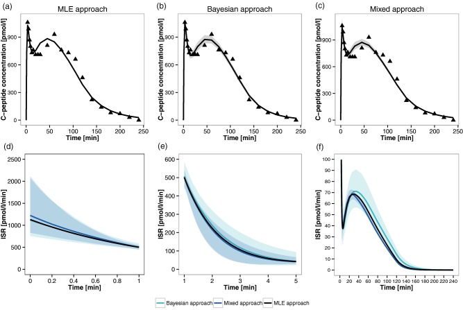
Individual fits for the insulin minimal model (MM) and reconstructed insulin secretion rate (ISR) profile. (a–c) The panels correspond to the three proposed approaches: maximum likelihood estimation (MLE) approach a, Bayesian approach b, and mixed approach c. The triangles represent individual C‐peptide (CP) concentration data, the solid line represents the model fit line, and the shaded gray area depicts the 95% confidence interval of the MM calculated without considering residual error variability. (d–f) Expected time course (solid line) and 95% confidence region (shaded area) of the ISR estimated via the three implemented approaches. Panels d, e, and f correspond to time intervals [0,1], [1,5], and [5,240] minutes, respectively.

Despite that this approach includes stochastic elements, such as interindividual variability or residual error, all the model parameters are considered as deterministic elements during estimation and simulation, making it unsuitable for uncertainty propagation among different models and hierarchical levels. This task will be faced in the next sections, in which Bayesian approaches are adopted.

Workflow results using a full‐Bayesian approach

Approach 2 was executed using WinBUGS as a target tool for estimation and simulation (see Figure 2 b). The posterior distribution of the M4 model population parameters was computed, and the relative point estimates and uncertainties were derived (see Table 1). All of them are consistent with the values reported using a different target tool (MCMC implemented via MATLAB).47 Trace plots (see Supplementary Figure S4), obtained via the coda R package, were used to assess the Markov Chain convergence to eventually set the burn‐in. In this case, chains were highly correlated. For this reason, to reduce autocorrelation and to save disk space, a thin of 10 was chosen to give an effective number of independent samples of at least 500 for each parameter. To check the effective number of independent samples, the R function effectiveSize (available in the coda R package) was used. As it was carried out for approach 1, VPCs were also performed (see Supplementary Figure S5); in this case, a custom R function was used, relying on the computed simulation profiles.

Stochastic simulations of M4 were performed to obtain the compartmental parameters and their precisions for the new subject. In these simulations, the priors on model parameters were replaced with the joint posterior distribution obtained after model identification, as (sampled) empirical distribution on all the model parameters. The point estimates of the compartmental parameters (with their 95% confidence intervals) for the new subject, reported in Supplementary Figure S6 and Table 1, were highly consistent with the values in the original work.47

The joint probability distribution of the compartmental parameters of the new subject (500 samples) was used as empirical prior for these parameters during MM estimation. Posterior distributions were obtained for all the MM parameters and the relative point estimates and uncertainties were computed (see Table 2), with results consistent with approach 1 and the original publication.44

The burn‐in and thinning values were chosen via trace plot (see Supplementary Figure S7) and effectiveSize function, as described above. The individual predicted vs. observed CP concentration plot is reported in Supplementary Figure S8.

The identified MM was simulated to obtain the predicted CP plasma concentration (see Figure 4 b) and ISR (see Figure 4 d–f) time course plots. As before, sensitivity indexes and ISR are consistent with the values obtained in the original work for this subject.44

Workflow results using a mixed MLE/Bayesian approach

Approach 3 is a combination of approaches 1 and 2 (see Figure 2 c). The compartmental parameters simulated with NONMEM in approach 1 (see Table 1) were used as fixed values during MM Bayesian estimation with WinBUGS. Point estimates and uncertainty of the MM parameters and sensitivity indexes in the new subject are reported in Table 1. As before, all of them were consistent with the values estimated in approaches 1 and 2, as well as the ones in the original publication.44 As in approach 2, predicted CP and ISR were obtained via stochastic simulations, which are reported in Figure 4 c and Figure 4 d–f. The numbers of burn‐in iterations, update iterations, and thin were chosen as described above (trace plots reported in Supplementary Figure S9).

Supported features of the WinBUGS plugin

Considering the models and performed tasks in approach 2, the support of a wide number of features was demonstrated, including: estimation and simulation tasks, population and single‐subject models, algebraic and ODE structural models, continuous and categorical covariates, time‐dependent forcing functions, multiple observations, IF‐THEN‐ELSE statements, correlated random effects, parametric and nonparametric (i.e., expressed with frequency table) or empirical (i.e., expressed through a list of samples) prior distributions. Specifically, our software plugin supports all the WinBUGS‐compatible probability distributions included in the ProbOnto ontology (version 2.0),50 which is used as a standard knowledge‐base in MDL and PharmML.

In addition to M4 and MM, the WinBUGS plugin was tested on a collection of about 200 additional models (list not reported), including different features of interest in pharmacometrics. Based on these tests, a full list of supported features is reported in Table 3. Compared to the WinBUGS plugin available in the IOF public release,33 the new version of the plugin has been robustified and now supports new features, as highlighted in Table 3.

Table 3.

List of modeling features supported by the Interoperability Framework with the WinBUGS plugin extension

Feature	Example	Limitations or assumptions
Multiple variability levels	UseCase1	Variability is supported on the population (prior), individual (between‐subject) and observation (residual) levels
Algebraic and ODEs models	UseCase1, UseCase2	ODE models are solved via PK/PD Model Library and WBDev. Initial time is always assumed to be zero.
IF‐THEN‐ELSE statements	UseCase1
Univariate and multivariate distributions from ProbOnto knowledge‐base	See Supplementary Information Appendix SB	Only the ones supported by WinBUGS*
Unary and binary operators	See Supplementary Information Appendix SA	Only the ones supported by WinBUGS*
Pairwise covariance and correlation encoding	UseCase1
Additive, proportional and combined observation error models	UseCase1	Only continuous outputs and structured expressions are supported: OBSERVATION = PREDICTION + f*EPS, with EPS distributed as a Normal and f depending on the error model*
Single, multiple independent observations and observations with multivariate distribution	M4	Only univariate and multivariate Normal distributions are supported
Multiple dosing	Simeoni2004
Multiple administration routes	UseCase4_1
NM‐TRAN data file	All models	Supported columns: ID, DV, DVID, EVID, MDV, AMT, CMT, SS, RATE, II, ADDL
Continuous and categorical covariates	UseCase5	All the covariates are assumed to be time‐dependent; continuous ones are linearly interpolated; constant interpolation is performed on categorical ones
Transformation of covariates, individual parameters, and observation models	UseCase5
PK macros	UseCase5
Univariate/multivariate empirical and nonparametric prior distributions	MM	Sample(s) (for empirical) and bin(s)‐probability (for nonparametric) values must be provided via external csv file
Structured (linear and general) expressions for individual parameters	UseCase1
Matrices and vectors	M4	They can only be used in population parameters and they cannot be used in IF‐THEN‐ELSE statements or ODEs*

MM, minimal model; ODE, ordinary differential equation; PK, pharmacokinetic; PK/PD, pharmacokinetic/pharmacodynamic.

To each feature, at least one model is associated as an example. The model names are referred to Modeling Description Language (MDL) files provided as Supplementary Information S1. For all the modeling features supported by MDL, the known limitations are listed too, specifying if they are due to the design of the WinBUGS plugin or to the WinBUGS target language itself (marked with *). Novel features, not supported in the previous version of the WinBUGS plugin (version 1.0, integrated into the official interoperability framework public release) are reported in bold.

DISCUSSION

Reproducibility and interoperability of model codes among different target languages and software tools have been demonstrated with a complex workflow, which has been executed via three different approaches combining several tools.

With approach 1, we have demonstrated how, in a single R script (Supplementary Information 2), users can estimate model parameters using NONMEM and do model qualification using PsN and Xpose. Although all the steps of the workflow could have been performed with the standalone versions of these software tools, writing an unbroken R script can significantly support the error‐free reproducibility of the carried out analysis, because all the task‐implementing commands can be included in a single file (e.g., fixing model parameters to the previously estimated values, reuse the same model for estimation, simulation, and VPC). Moreover, the output of all the performed tasks was saved in an SO file, supporting subsequent result comparisons among different target tools (e.g., through the application of standard Xpose graphic functions).

The other key advantage of the IOF features is interoperability, which allows the reuse of the same data and/or model encoding, for executing the desired tasks via different target languages and tools. This feature has been demonstrated in approaches 2 and 3, in which the code (model and data) used in approach 1 has been easily reused in a Bayesian setting, thanks to the modular structure of the MDL. In fact, MDL objects can be grouped in different ways within IOF to execute different tasks, even in different software tools.

Further, with approaches 2 and 3, we have demonstrated the possibility of executing Bayesian estimation and stochastic simulation tasks in the IOF via WinBUGS by using only MDL and R scripts (Supplementary Information 2). Both the estimation and simulation results were stored in an SO file, like in approach 1. Therefore, interoperability and standardization have also been highlighted at the level of result management by the possibility of applying, in all the tested approaches, “universal” functions to SO files, without taking into account which software generated results and which was the specific format for storing them. That was made possible thanks to the standardized format of the IOF outputs (SO) that promotes interoperability and enables direct comparisons among results coming from different target tools and/or tasks. For instance, an easy to do comparison between the confidence bands around the ISR estimates (see Figure 4 d–f) highlights, in this case, that the central tendency of the reconstructed ISR time course is comparable among the different approaches (with only a slight overestimation of the ISR in the MLE approach), whereas the propagated variability, represented with the 95% confidence interval around the central tendency, increases from the mixed approach to the full‐Bayesian approach, as expected. It is worth noting that the confidence region of the mixed approach is completely included within one of the full‐Bayesian approaches only after the first 5 minutes, whereas, in the first two phases, the differences between the confidence regions are quite limited.

Finally, the integration of WinBUGS within the DDMoRe IOF, through the WinBUGS plugin, has even reduced the complexity of directly implementing PK/PD models, which are normally encoded in the standalone version of WinBUGS by combining in a not trivial way BUGS code and Component Pascal languages. In particular, modelers can encode the desired MDL files by writing them from scratch, taking advantage of the MDL‐IDE and a detailed user guide, or modifying existing model files, such as the ones available in the DDMoRe Model Repository. The modular structure of MDL (see example in Figure 3) facilitates such a task, by enabling the reuse of blocks from existing model files, which may be modified only in terms of, for example, data or prior distribution of specific parameters. Any MDL file can be executed via user‐defined R scripts, like the ones programmed in this work and included in the Supporting Information zip files. Once executed via specific R functions, MDL can successfully serve as a BUGS/Pascal translation system, because every execution creates and makes available to users all the model files in the target code. If needed, the resulting files can be integrated, modified, and executed by users in standalone WinBUGS.

The work herein presented relied on the WinBUGS plugin available functionality and extensibility; however, the lessons learned could facilitate the development of future DDMoRe IOF plugins for other promising Bayesian tools, such as Stan.

The plugin used in this work is publicly available and supports a plethora of pharmacometric modeling features (Table 3). It is expected to significantly facilitate Bayesian model encoding, execution, and results comparison among different estimation/simulation tools by addressing reproducibility and interoperability, two long‐standing problems in pharmacometric modeling, as well as by “making easy” the encoding of PK/PD models in WinBUGS. This can substantially contribute to boost the adoption of the Bayesian approach in pharmacometrics.

Source of Funding

This study has received support from the Innovative Medicines Initiative Joint Undertaking under grant agreement number 115156, resources of which are composed of financial contributions from the European Union's Seventh Framework Programme (FP7/2007–2013) and European Federation of Pharmaceutical Industries and Associations (EFPIA) companies’ in‐kind contribution. The DDMoRe project is also financially supported by contributions from Academic and SME partners.

Conflict of Interest

The authors declared no conflict of interest.

Author Contributions

C.L., E.B., L.P., and P.M. wrote the manuscript. P.M. designed the research. C.L., E.B., L.P., P.T., M.S., S.M., and P.M. performed the research. E.B., L.P., and P.M. analyzed the data.

Supporting information

SUPPLEMENTARY Figure S1 Histograms of bootstrap M0 parameter estimates with normal density curves obtained via the maximum likelihood estimation (MLE) approach.

SUPPLEMENTARY Figure S2 Visual predictive check (VPC) plots of M0 obtained via the maximum likelihood estimation (MLE) approach.

Red solid line, median of observed data; red dashed line, 95% confidence interval (CI) of observed data; red shaded area, 95% CI around median of simulated data; blue shaded area, 95% CI around 95% prediction interval (PI) of simulated data for short half‐life (a), amplitude fraction (b), long half‐life (c), and volume of distribution (d).

SUPPLEMENTARY Figure S3 Goodness‐of‐fit (GOF) plots of the insulin minimal model (MM) obtained via the maximum likelihood estimation (MLE) approach. Observations vs. individual predictions (a), individual weighed residuals vs. individual predictions (b), weighted residuals vs. time (c), observations/predictions vs. time (d).

SUPPLEMENTARY Figure S5 Visual predictive check (VPC) plots of M4 obtained via the full‐Bayesian approach. Red solid line, median of observed data; red dashed line, 95% confidence interval (CI) of observed data; red shaded area, 95% CI around median of simulated data; blue shaded area, 95% CI around 95% prediction interval (PI) of simulated data for short half‐life (a), amplitude fraction (b), long half‐life (c), and volume of distribution (d).

SUPPLEMENTARY Figure S6 The C‐peptide (CP) kinetic parameters for a new subject. The point estimates obtained via the maximum likelihood estimation (MLE) approach are denoted by a solid line and the 95% confidence intervals obtained via the full‐Bayesian approach by a colored zone (with the median denoted by a solid line).

SUPPLEMENTARY Figure S8 Observations vs. individual predictions plot of the insulin minimal model (MM) obtained via the full‐Bayesian approach.

SUPPLEMENTARY Table S1 Bootstrap parameter estimates of M0 obtained via the maximum likelihood estimation (MLE) approach.

Supporting Methods, Figures S10‐S11

Model Code

R Script

SUPPLEMENTARY MATERIAL

References

- 1. Leil, T.A. A Bayesian perspective on estimation of variability and uncertainty in mechanism‐based models. CPT Pharmacometrics Syst. Pharmacol. 3, e121 (2014). [DOI] [PMC free article] [PubMed] [Google Scholar]
- 2. Migon, H.S. , Gamerman, D. & Louzada F. Statistical Inference: An Integrated Approach, Second Edition (Chapman and Hall/CRC Press, Baton Rouge, FL, 2014). [Google Scholar]
- 3. Malakoff, D. Bayes offers a ‘new’ way to make sense of numbers. Science 286, 1460–1464 (1999). [DOI] [PubMed] [Google Scholar]
- 4. Best, N.G. , Tan, K.K. , Gilks, W.R. & Spiegelhalter, D.J. Estimation of population pharmacokinetics using the Gibbs sampler. J. Pharmacokinet. Biopharm. 23, 407–435 (1995). [DOI] [PubMed] [Google Scholar]
- 5. Gelman, A. , Carlin, J.B. , Stern, H.S. , Dunson, D.B. Vehtari, A. & Rubin, D.B. Bayesian Data Analysis Third Edition (Chapman and Hall/CRC Press, Boca Raton, FL, 2013). [Google Scholar]
- 6. Lunn, D.J. , Thomas, A. , Best, N. & Spiegelhalter, D. WinBUGS – a Bayesian modelling framework: concepts, structure, and extensibility. Stat. Comput. 10, 325–337 (2000). [Google Scholar]
- 7. MRC Biostatistics Unit . The BUGS Project. WinBUGS. <http://www.mrc-bsu.cam.ac.uk/software/bugs/the‐bugs‐project‐winbugs/> (2007).
- 8. Lunn, D.J. , Spiegelhalter, D. , Thomas, A. & Best, N. The BUGS project: evolution, critique and future directions. Stat. Med. 28, 3049–3067 (2009). [DOI] [PubMed] [Google Scholar]
- 9. MRC Biostatistics Unit . The BUGS Project. OpenBUGS. <http://www.openbugs.net/w/FrontPage> (2007).
- 10. Carpenter, B. et al Stan: a probabilistic programming language. J. Stat. Softw. 76, 1–43 (2017). [DOI] [PMC free article] [PubMed] [Google Scholar]
- 11.Stan software. <http://mc-stan.org/> (2017).
- 12. Plummer, M. JAGS: a program for analysis of Bayesian graphical models using Gibbs sampling. Proceedings of the 3rd International Workshop on Distributed Statistical Computing, Vienna, Austria, March 20–22, 2003.
- 13. JAGS , another Gibbs Sampler. <http://mcmc-jags.sourceforge.net/> (2017).
- 14. Beal, S.L. , Sheiner, L.B. , Boeckmann, A.J. & Bauer, R.J. NONMEM User's Guides (1989–2009). Technical report (Icon Development Solutions, Ellicott City, MD, 2009).
- 15. Bauer, R.J. & Ludden, T.M. Improvements and new estimation methods in NONMEM 7 for PK/PD population analysis. Abstract #1516. <http://www.page-meeting.org/?abstract=1516> (2009).
- 16. Gilks, W.R. , Richardson, S. & Spiegelhalter, D. Markov Chain Monte Carlo in practice (Chapman and Hall, London, UK, 1996).
- 17.WinBUGS Development Interface website (WBDev). <http://winbugs-development.mrc-bsu.cam.ac.uk/> (2004).
- 18.BUGSModelLibrary is a prototype PKPD model library for use with WinBUGS 1.4.3. <https://bitbucket.org/metrumrg/bugsmodellibrary/wiki/Home> (2015).
- 19.Welcome to Metrum Institute. <http://metruminstitute.org/> (2014).
- 20. Gillespie, W.R. Bayesian pharmacometric modeling with BUGS, NONMEM, and Stan. Presented at the Bayes 2015 Basel meeting, May 22, 2015. <http://www.bayes-pharma.org/wp-content/uploads/2014/10/BayesianPmetricsBAYES2015.pdf> (2015).
- 21. Oberon Microsystems . BlackBox. <http://www.oberon.ch/blackbox.html> (2001).
- 22. Borella, E. et al Evaluation of software tools for Bayesian estimation on population models with count and continuous data. Abstract 3452 <http://www.page-meeting.org/?abstract=3452> (2015).
- 23. Gastonguay, M.R. , Gillespie, W.R. & Bauer, R.J. Comparison of MCMC simulation results using NONMEM 7 or WinBUGS with the BUGSModelLibrary. Abstract 1762 <http://www.page-meeting.org/?abstract=1762> (2010).
- 24. Bauer, R.J. NONMEM Users Guide. Introduction to NONMEM 7.4.1. <https://nonmem.iconplc.com/nonmem741/nm741.pdf> (2017)
- 25. Bauer, R.J. , Guzy, S. & Ng C. A survey of population analysis methods and software for complex pharmacokinetic and pharmacodynamic models with examples. AAPS J. 9, E60–E83 (2007). [DOI] [PMC free article] [PubMed] [Google Scholar]
- 26. Duffull, S.B. , Kirkpatrick, C.M. , Green, B. & Holford N.H. Analysis of population pharmacokinetic data using NONMEM and WinBUGS. J. Biopharm. Stat. 15, 53–73 (2005). [DOI] [PubMed] [Google Scholar]
- 27. Zhou, Z. , Rodman, J.H. , Flynn, P.M. , Robbins, B.L. , Wilcox, C.K. & D'Argenio, D.Z. Model for intracellular lamivudine metabolism in peripheral blood mononuclear cells ex vivo and in human immunodeficiency virus type 1‐infected adolescents. Antimicrob. Agents Chemother. 50, 2686–2694 (2006). [DOI] [PMC free article] [PubMed] [Google Scholar]
- 28. Dubois, V.F. et al Assessment of interspecies differences in drug‐induced QTc interval prolongation in cynomolgus monkeys, dogs and humans. Pharm. Res. 33, 40–51 (2016). [DOI] [PMC free article] [PubMed] [Google Scholar]
- 29. Lunn, D.J. , Best, N. , Thomas, A. , Wakefield, J. & Spiegelhalter, D. Bayesian analysis of population PK/PD models: general concepts and software. J. Pharmacokinet. Pharmacodyn. 29, 271–307 (2002). [DOI] [PubMed] [Google Scholar]
- 30.PKBugs: an efficient interface for population PK/PD within WinBUGS. <http://winbugs-development.mrc-bsu.cam.ac.uk/pkbugs/home.html> (2004).
- 31.WinBUGS Development website. Pharmaco interface. <http://winbugs-development.mrc-bsu.cam.ac.uk/> (2004).
- 32. Kokash, N. , Moodie, S.L. , Smith, M.K. & Holford, N. Implementing a domain‐specific language for model‐based drug development. Procedia Comput. Sci. 63, 308–316 (2015). [Google Scholar]
- 33. Drug Disease Model Resources (DDMoRe) . Official Release – Interoperability Framework. <http://www.ddmore.eu/official-release-interoperability-framework> (2016).
- 34. Harnisch, L. , Matthews, I. , Chard, J. & Karlsson, M.O. Drug and disease model resources: a consortium to create standards and tools to enhance model‐based drug development. CPT Pharmacometrics Syst. Pharmacol. 2, e34 (2013). [DOI] [PMC free article] [PubMed] [Google Scholar]
- 35.Drug Disease Model Resources (DDMoRe) Foundation. <https://www.ddmore.foundation/> (2016).
- 36. Swat, M.J. et al Pharmacometrics Markup Language (PharmML): opening new perspectives for model exchange in drug development. CPT Pharmacometrics Syst. Pharmacol. 4, 316–319 (2015). [DOI] [PMC free article] [PubMed] [Google Scholar]
- 37. Terranova, N. et al Standardized output: flexible and tool‐independent storage format of typical M&S results. Abstract 3599 <http://www.page-meeting.org/?abstract=3599> (2015).
- 38. Smith, M.K. et al Model Description Language (MDL): a standard for modelling and simulation. CPT Pharmacometrics Syst. Pharmacol. 6, 647–650 (2017). [DOI] [PMC free article] [PubMed] [Google Scholar]
- 39. R Core Team . R: a language and environment for statistical computing. R Foundation for Statistical Computing, Vienna, Austria. <https://www.R-project.org/> (2015).
- 40. Waltemath, D. & Wolkenhauer, O. How modeling standards, software, and initiatives support reproducibility in systems biology and systems medicine. IEEE Trans. Biomed. Eng. 63, 1999–2006 (2016). [DOI] [PubMed] [Google Scholar]
- 41. Smith, L. , Swat, M.J. & Barhak, J. Sharing formats for disease models. Proceedings of the Summer Computer Simulations Conference (SCSC). Article 5, Montreal, Quebec, Canada, July 24–27, 2016.
- 42. Toffolo, G. , De Grandi, F. , Cobelli, C. Estimation of beta‐cell sensitivity from intravenous glucose tolerance test C‐peptide data. Knowledge of the kinetics avoids errors in modeling the secretion. Diabetes 44, 845–854 (1995). [DOI] [PubMed] [Google Scholar]
- 43. Cretti, A. et al Assessment of beta‐cell function during the oral glucose tolerance test by a minimal model of insulin secretion. Eur. J. Clin. Invest. 31, 405–416 (2001). [DOI] [PubMed] [Google Scholar]
- 44. Magni, P. , Sparacino, G. , Bellazzi, R. , Toffolo, G.M. & Cobelli, C. Insulin minimal model indexes and secretion: proper handling of uncertainty by a Bayesian approach. Ann. Biomed. Eng. 32, 1027–1037 (2004). [DOI] [PubMed] [Google Scholar]
- 45. Polonsky, K.S. et al Use of biosynthetic human C‐peptide in the measurement of insulin secretion rates in normal volunteers and type I diabetic patients. J. Clin. Invest. 77, 98–105 (1986). [DOI] [PMC free article] [PubMed] [Google Scholar]
- 46. Van Cauter, E. , Mestrez, F. , Sturis, J. & Polonsky K.S. Estimation of insulin secretion rates from C‐peptide levels. Comparison of individual and standard kinetic parameters for C‐peptide clearance. Diabetes 41, 368–377 (1992). [DOI] [PubMed] [Google Scholar]
- 47. Magni, P. , Bellazzi, R. , Sparacino, G. & Cobelli, C. Bayesian identification of a population compartmental model of C‐peptide kinetics. Ann. Biomed. Eng. 28, 812–823 (2000). [DOI] [PubMed] [Google Scholar]
- 48.Drug Disease Model Resources (DDMoRe) Model Repository. <http://repository.ddmore.eu/> (2017).
- 49. Shapiro, E.T. , Tillil, H. , Rubenstein, A.H. & Polonsky, K.S. Peripheral insulin parallels changes in insulin secretion more closely than C‐peptide after bolus intravenous glucose administration. J. Clin. Endocrinol. Metab. 67, 1094–1099 (1988). [DOI] [PubMed] [Google Scholar]
- 50. Swat, M.J. , Grenon, P. & Wimalaratne S.M. ProbOnto: ontology and knowledge base of probability distributions. Bioinformatics 32, 2719–2721 (2016). [DOI] [PMC free article] [PubMed] [Google Scholar]
Associated Data
This section collects any data citations, data availability statements, or supplementary materials included in this article.
Supplementary Materials