Deep learning and virtual drug screening

Abstract

Current drug development is still costly and slow given tremendous technological advancements in drug discovery and medicinal chemistry. Using machine learning (ML) to virtually screen compound libraries promises to fix this for generating drug leads more efficiently and accurately. Herein, we explain the broad basics and integration of both virtual screening (VS) and ML. We then discuss artificial neural networks (ANNs) and their usage for VS. The ANN is emerging as the dominant classifier for ML in general, and has proven its utility for both structure-based and ligand-based VS. Techniques such as dropout, multitask learning and convolution improve the performance of ANNs and enable them to take on chemical meaning when learning about the drug-target-binding activity of compounds.

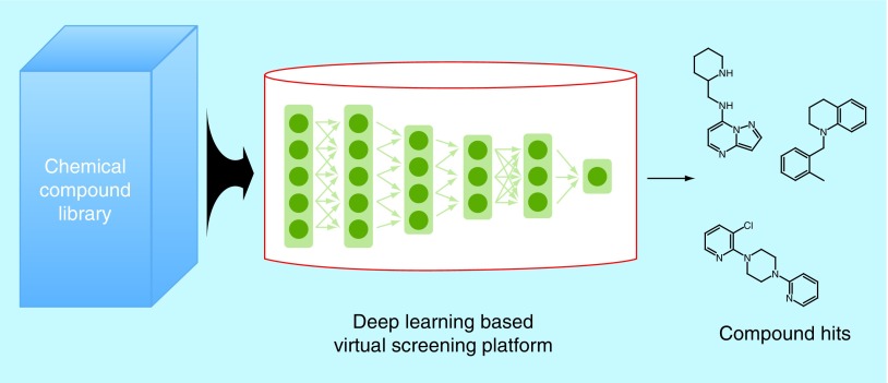
Graphical abstract

Virtual screening

Virtual screening (VS) has emerged in recent years as a way to expedite drug development – a process that takes years and, as of 2014, costs an estimated US$2.87 billion [1]. VS takes place at the early discovery phase, in which the most promising lead compounds are found in large chemical databases. This used to primarily be done through high-throughput screening (HTS), an in vitro method involving conducting assays on thousands of compounds. While new technologies have made HTS less time consuming, it is only through virtual methods that the yield of initial screens can be greatly increased. Instead of physically testing every compound in a given library, VS entails the computation of the compounds’ properties in order to predict which will be most favorable to bind to the desired drug target. There are two types of VS: structure-based virtual screening (SBVS) and ligand-based virtual screening (LBVS). SBVS uses the 3D structure of a compound to predict its drug-target-binding affinity. One common way to do this is through docking, in which the compound and target are placed together in a simulation. Calculations of chemical potential influence the output of the scoring function, which is a metric of how probable it is for the two molecules to noncovalently bind [2]. One of the most widely used docking programs is AutoDock Vina [3]. On the other hand, LBVS uses molecular and chemical properties (often represented by molecular fingerprints [4] or molecular descriptors [5,6]) to check similarity between a test compound and a known ligand of the target. LBVS is based on the idea that compounds with similar properties will have similar target-binding activity [7].

No matter whether the VS is structure based or ligand based (or uses a combination of both), pre- and postprocessing is required. Even though the virtual nature of VS enables researchers to test as many compounds as they would like from public chemogenomics libraries (such as ChemBL [8], PubChem [9] or ZINC [10]) or private libraries from pharmaceutical companies, it is crucial to filter before conducting the actual screen. Filtering often involves removing duplicate/excessively similar compounds, as well as compounds that are unlikely to be effective drugs. The latter is determined through established metrics like Lipinski's Rule of Five [11] or rules for predicted drug leadlikeness [12].

Machine learning

The power of VS is bolstered with the use of machine learning (ML). Rather than conducting computationally expensive simulations or exhaustive similarity searches, a good ML model is able to screen for predicted hits much faster. In order to understand how ML can be applied to VS, one must first have a solid grasp of what ML is.

ML is a method of achieving artificial intelligence, the ability of a machine to implement intelligent tasks. The core idea behind ML is that, instead of writing an algorithm to turn inputs into outputs, it is possible to train a classifier that generates some sort of algorithm based on pairs of inputs and outputs, which can then be used on unseen inputs to provide new outputs. In the context of VS, this means that we can create a model which predicts if a given compound will bind to a given target after being trained on a dataset containing both compounds that are known to bind and compounds that are known to not bind. Finding such a model is not easy. A balance must be struck between accuracy on the training set and generalizability to unseen data. If too much weight is given to performance on the training data, then there is risk of overfitting, which will lead to poor performance on test data. However, poor performance can also come from an underfitted classifier. The strategy for balancing these extremes is called the structural risk minimization principle [13]. Different classifiers have different ways of following structural risk minimization.

Regardless of the type of classifier being used, it is crucial to estimate its level of accuracy. Accuracy can be tested by checking the predictions the trained classifier makes on a test set of inputs against their real outputs – a process which is called validation. Because validating a classifier on the same data on which it was trained will always lead to an overestimate of its accuracy, validation must use a test set distinct from the training set. When the test set comes from the same cohort sample as the training set, the validation is said to be internal. External validation is when the training set and test set are from different cohorts. While external validation gives a better assessment of a model's performance on unseen data, it is not always possible to amass enough data collected from different cohorts. For this reason, most ML models are initially evaluated using internal validation [14]. The difference between external and internal validation is visually represented in Figure 1.

Figure 1. . Internal versus external validation.

This is a visual representation of the conceptual difference between internal and external validation. The arrow points from the data to be validated to the data used for validation.

Using internal validation requires splitting available data into a training set and a testing set. There are two ways of doing this. If there is a large quantity of available data, the data can often simply be split randomly into two groups. A validation set may be used to train the model and to optimize hyperparameters, the parameters set before the learning process is initiated [15,16]. VS is an exception for random selection, as it leads to overly optimistic prospective predictions [17,18]. A structural split is appropriate in this context [19,20]. Because classifier accuracy is predominantly dependent on how large the training set is, it is common to designate 70–80% of available data as the training set, with the remaining 20–30% being the testing set. However, in some cases, this method of splitting causes the training and testing sets to not be satisfactorily large enough. This is when k-fold cross-validation becomes useful. The dataset is randomly split into k distinct partitions (with k customarily being set to 5 or 10). One partition is chosen to be the test set, and the remaining k-1 combine to form the training set to build a classifier. This classifier is evaluated with the test set. This process is done a total of k times (so that each partition serves as the test set exactly once), and the classifier that had the best performance is chosen as the final classifier to be used on unseen data.

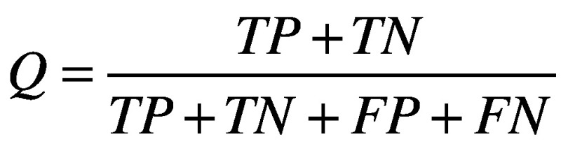
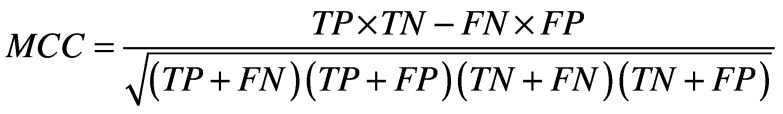
There are several standard metrics for evaluating a classifier's performance on a given test set. These are based on quantities calculated from the confusion matrix, which relates true positives (TP), false positives (FP), true negatives (TN) and false negatives (FN). Among these are sensitivity (Equation 1) [21], specificity (Equation 2) [21], accuracy (Equation 3) [21] and the Matthews’ correlation coefficient (Equation 4) [22]. The closer all of these values are to 1, the better. Plotting specificity against (1 - sensitivity) yields the receiver operating characteristic curve. Taking the area under the receiver operating characteristic (AUC) is another measure of performance; an AUC of 0.5 means the classifier is behaving as if it were assigning classifications randomly, while an AUC of 1 means the classifier is optimally accurate. One final performance indicator that is specifically used for VS is the Boltzmann-enhanced discrimination of receiver operating characteristic, which is tailored to better evaluate performance of classifiers which rank predicted active compounds [23].

(Equation 1)

(Equation 2)

(Equation 3)

(Equation 4)

There are many parameters (stopping thresholds, number of trees or layers, length of training epoch, etc.) that need to be set for various types of classifiers. Rather than blindly picking values for these parameters and hoping for the best, it is typical for researchers designing the ML architecture to construct multiple models, each with slightly different parameter settings and compare their internal validation scores to choose the best.

Once a trained and evaluated ML model has been created and deemed satisfactory, it can be used to conduct VS on extremely large chemogenomic libraries. The highest scoring compounds are called hits, and are subject to in vitro testing in order to verify if they have favorable target-binding activity. The yield of these tests is much higher than a normal HTS, since the ML model has already predicted binding. From this point, the most promising compounds (called leads) may be further developed and tested, hopefully becoming produced drugs. This ML for VS workflow is summarized in Figure 2.

Figure 2. . A block diagram of the optimal workflow for machine learning-based virtual screening.

Artificial neural networks

There are many different types of classifiers, each with their own advantages and disadvantages. In this review, we will focus on one classifier that is becoming massively popular and has proven to be very effective: the artificial neural network (ANN).

ANNs were one of the original proposed forms of ML, with their first simple manifestation being Rosenblatt's perceptron in 1958 [24]. As can be inferred from their name, ANNs began as attempted reproductions of the interactions between neurons in the brain. They comprise layers of nodes, which together transform the input into output through weights, biases and activation functions. There are three types of layers in the classic ANN: the input layer, the hidden layer and the output layer. The input layer and output layer are representations of the input to and output of the classifier, respectively. The hidden layers have a less intuitive name, but are conceptually simple; these are the layers between the input and output layers that transform the data in order to make predictions. An ANN can have any number of hidden layers. Figure 3 shows the relationship that ANNs have to other artificial intelligence concepts. Note that ANNs are a form of deep learning (DL). DL is a subset of ML in which inputs are successively transformed into alternate representations that better allow for extraction of patterns. The ‘deepness’ in an ANN comes through its hidden layers – the more hidden layers an ANN has, the more intermediate representations it encodes and the deeper it is. Another kind of DL is the deep belief network, which differs from an ANN in that it is unsupervised.

Figure 3. . Representation of the hierarchy and relationship between different artificial-related concepts.

These concepts exist as subsets of each other.

The typical ANN is fully connected, which means that every node in the input and hidden layers is connected to every other node in the next layer (the exception to this when convolution is used, which is explained below). The data must be transformed between every layer (otherwise the output would be identical to the input). The weight matrix of each hidden layer (and the output layer) conducts a linear transformation on the previous layer's data, and the bias term can add a constant to this result. The resulting numbers are fed into an activation function in order to transform the data nonlinearly (since having only successive linear transformations could be accomplished with a single linear transformation from input to output, with no need for any hidden layers).

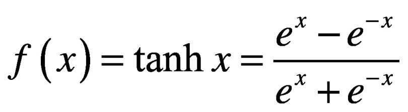
There are many types of activation functions, which are applicable in different contexts. If one wants to simply use a linear transformation for a given layer, they can use a linear or identity activation function. More often though, nonlinear transformations are required. One typical nonlinear activation is the sigmoid function. Sigmoid functions are continuous and differentiable everywhere (which is preferable for gradient descent), and are bounded (which is preferable for classification). Two common sigmoid activations are the logistic (Equation 5) and hyperbolic tangent (Equation 6) functions. Because these yield strictly positive results, the model is usually interpreted with 0 representing false/inactive and 1 representing true/active. If the model is being used for regression (i.e., is producing a numerical output rather than predicting from a finite number of classes), then it is important that none of the real outputs are negative, since it will be impossible for the model to produce these. Another nonlinear activation is the rectified linear unit (ReLU; Equation 7) [25]. ReLUs are similar to sigmoids in that they cannot propagate negative values, but unlike sigmoids, they do not have an upper bound. Because of this, they are called ‘non-saturating.’ While both sigmoids and ReLUs are useful in various situations, it has been shown that training is generally faster [26] and the resulting models are generally more accurate [27], when ReLUs are used in hidden layers. The vast majority of ANNs for VS presented later in this review exclusively use ReLU activations.

(Equation 5)

(Equation 6)

(Equation 7)

The idea of the ANN has been around for over 50 years and advancements in both algorithms and hardware have greatly increased their performance, causing them to become more widespread over time. In 1986, Rumelhart et al. popularized back-propagation [28], which is a process that uses sequential gradient calculations to optimize the weights in a network. Specifically, this involves calculating the partial derivative of the chosen objective function (which is the prediction's loss) with respect to each weight. Once these gradients are found, the weights can be updated so that the loss function approaches a local minimum. If all data points are used for updating with back-propagation, this process is called gradient descent. However, because reaching a local minimum involves multiple back-propagation calculations, using the entire training set can take too much time. This can be remedied by instead using stochastic gradient descent (SGD), in which weight updates are made after the gradient calculation of only a single, randomly selected point. The stochastic nature of SGD means that some noise will be introduced into the weight setting, but the technique is overall still very effective and is widely used. See Figure 4 for a visual representation.

Figure 4. . Stochastic gradient descent compared with gradient descent.

A number of algorithmic breakthroughs happened throughout the late 2000s, such as unsupervised pretraining in 2006 [29]. As implied by the name, unsupervised pretraining involves calculation prior to SGD in order to initialize weights more effectively than simply setting them at random. In 2013, Sutskever et al. effectively demonstrated the importance of momentum [30], which is an improved version of back-propagation where local minima are reached faster by retaining information about previous updates. Momentum also adapts the size of updates, so that ‘steep’ gradients do not cause inordinately large changes (which could lead to overshooting a local minimum) and ‘flat’ gradients do not cause inordinately small ones (which could prevent sufficient progress to the minimum within the allotted training time). In 2014, dropout was debuted [31]. Dropout is used to improve the generalizability of an ANN. Each hidden node is given a probability of being ‘dropped’ by the network during training, meaning that its output is set to zero regardless of input. This means that no single node can dominate classification, which would usually lead to overfitting. Additionally, because different nodes are dropped with each iteration through the training data, the resulting network can, in simplified terms, be seen as analogous to the average of several slightly different networks [32].

These improvements, together with the all-around increase in computation speed and the increased use of graphics processing units (GPUs) to enhance performance [26,33,34], have given ANNs the boost needed to reach the level of popularity within the ML community that they have today.

A term frequently associated with ANNs is convolution. ANNs which use convolution are called Convolutional Neural Networks (often shortened to CNNs, or ConvNets). Convolutional layers are not fully connected, but rather pass a fixed-size filter over neighboring nodes throughout the input. This significantly cuts down the number of weights that need to be optimized by back-propagation, and has the added benefit of being able to detect similar features that appear throughout the data. Because of this, CNNs are typically associated with image classification [26].

The convolutional layers in CNNs are often followed by max-pooling layers, then by the typical fully connected layers to precede the output (Figure 5). The pooling layer reduces the size of the subsequent layer by only passing forward the highest value in every adjacent cluster of a certain number of nodes – for example, a size five pooling layer will pass on the maximum value of every group of five adjacent nodes. Doing this helps reduce noise. Strong current applications of CNNs, a class of ANNs, include natural language processing [35], object detection [36], visual tracking [37] and semantic segmentation [38].

Figure 5. . Example architecture of a Convolutional Neural Network.

Dropout would involve dropping certain nodes that are illustrated within the layers.

One last important term to know is multitask learning (MTL) [39,40]. While MTL is not as widespread of a buzzword as DL and convolution, it is just as prevalent in VS research and important to understand. The traditional ML classifier uses what is called single-task learning, which means that it is trained on one specific task. However, it is often more effective to train on multiple, related tasks. This is due to inductive bias, which says that learning similar tasks together is easier than learning them separately, even if they are very complicated. In the context of VS, the related tasks are usually a compound's potential binding activity to different targets. MTL is effective here because while different targets bind to different ligands, the laws of physics and chemistry are constant. MTL is implemented in ANNs by training shared hidden layers on multiple different tasks, with different output layers determining the predicted result for an individual task in testing, as represented by Figure 6. This helps keep the network generalizable by preventing it from becoming overly specialized toward a particular target. MTL is also commonly implemented in k-nearest neighbors (kNN), another ML technique. Some researchers have used MTL with kNN for VS [41].

Figure 6. . Visual representation of multitask learning.

ANNs in VS

In comparison studies, ANNs have outperformed other ML classifiers in conducting VS. In 2014, Dahl et al. compared quantitative structure–activity relationship (QSAR)-ANNs with the more dominant ML classifier for VS at the time, Random Forests. They found that the ANNs mostly outperformed the Random Forests, and that those which employed MTL outperformed those trained on a single task [42]. These findings are supported by a more comprehensive 2017 study conducted by Lenselink et al. The researchers directly compared the screening performance of deep neural networks with varying architectures: Support Vector Machines, Random Forests, Naive Bayes classifiers and Logistic Regression models. The ANNs all outperformed the other classifier types with regard to standardized methods of accuracy evaluation (Boltzmann-enhanced discrimination of receiver operating characteristic and Matthews’ correlation coefficient). The researchers also found that, among the ANNs, the ones with MTL were more accurate than the ones without [43]. In 2014, Unterthiner et al. demonstrated the efficacy of DL to be superior to seven target predictor methods, including commercial and ML predictors, on the ChEMBL database [44].

Now that we have explained how ANNs and CNNs work, and presented evidence that these classifiers are among the best for conducting VS, we will conclude this review with a broad sampling of recent research utilizing ANNs for drug discovery. This is by no means comprehensive, but should provide a good overview of the specific ways in which ANNs are implemented in VS. It should also be noted that there is a whole body of work utilizing neural networks in biological modeling predating the research to be presented [45–50].

ANNs have most commonly been used for LBVS. In these studies, QSAR [51] information is often used as the input information about each compound, with the training data being known active and inactive compounds. If the trained ANN shows satisfactory performance in validation, it is then used on large, untested chemical databases. The resulting hits are usually further tested with docking or in vitro assays. One example of QSAR-ANN is Prakash et al.'s 2013 study [52], which used this type of ML to search for compounds that are cytotoxic to human breast cancer cells. Their model found five compounds with predicted target-binding activity that was validated by non-VS tests. Similarly, Bilsland et al. [53] used an ANN to screen for senescence-inducing compounds, using known agonists and molecular descriptor data. Their model produced 147 hits from a screening library of 2 million compounds. These hits underwent in vitro assays until one compound was identified as the most favorable for further development.

QSAR-ANN has also been used in ensemble methods, which are systems that use multiple types of ML classifiers to make more robust predictions. For example, MLViS [54], an online VS tool developed in 2015, utilizes ANNs in addition to Naive Bayes, kNN, Decision Trees, Support Vector Machines and Random Forests. This particular ensemble model began by training and internally evaluating 23 classifiers of these types, then was launched for production with the ten most accurate trained models.

Though less prevalent, SBVS using ANNs have also been conducted. Instead of molecular descriptor data, these models are trained with structural information. The upside of this is that it is no longer necessary to have prior knowledge of active and inactive compounds. We will discuss two very different examples of ANNs for SBVS. The first of these is a deep ANN created by Ashtawy and Mahapatra in 2018 [55]. They initially constructed three distinct boosted Decision Trees to use compounds’ structures to predict target binding pose, binding affinity and classification of activity or inactivity. However, since these tasks are closely related, this is a prime situation for implementing MTL. The researchers’ ANN incorporates a shared hidden architecture to extract features useful for all three tasks, then later has additional task-specific layers which lead to each task's output. Tests showed that the multitask deep neural net was just as accurate as or more accurate than single-task learning models and traditional docking.

Another ANN model for SBVS is AtomNet™ [56], developed in 2015 by Atomwise, Inc. Like the previous example, this ANN uses structural information to extract features that can predict novel binding compounds. However, instead of using MTL, AtomNet uses convolution. After training, the filters of the resulting CNN were shown to be detecting chemical functional groups, which are important factors in a compound's binding ability. This contributes to AtomNet's effectiveness, and when it was compared with docking methods, it significantly outperformed them. See Table 1 for a breakdown of the recent studies explained in this section.

Table 1. . Recent research utilizing artificial neural networks for drug discovery.

Study	(year)	Method	Achievement	Ref.
Prakash et al.	(2013)	QSAR-ANN	Found CID_73621, CID_16757497, CID_301751, CID_390666 and CID_46830222 to be cytotoxic to human breast cancer cells	[52]
Bilsland et al.	(2015)	QSAR-ANN	Screened for senescence-inducing compounds and found 147 hits from a screening library of 2 million compounds. CB-20903630 was viewed as most favorable for further development	[53]
Korkmaz et al.	(2015)	ANNs in addition to Naive Bayes, kNN, Decision Trees, Support Vector Machines and Random Forests	Online VS tool utilizing most accurate models from a tested broader selection	[54]
Ashtawy and Mahapatra	(2018)	MTL, ANN	Proposed a novel multitask deep neural network capable of simultaneously predicting binding pose, binding affinity and classification of activity that performs better than conventional scoring functions	[55]
Wallach et al.	(2015)	DCNN	Introduced a DCNN designed to predict the bioactivity of small molecules for drug discovery applications while outperforming previous docking approaches	[56]

ANN: Artificial neural network; DCNN: Deep convolutional neural network; kNN: k-Nearest neighbor; MTL: Multitask learning; QSAR: Quantitative structure-activity relationship; VS: Virtual screening.

Conclusion

As drug development becomes a slower and more expensive process, it is imperative to seek out emergent tools to make it more efficient. VS has proven to be a quick, high-yield method of finding lead compounds that have the potential to become effective drugs. While VS can take many forms, ML-based screens are among the least computationally expensive and have experienced significant success. Many different classifiers are possible for application to VS, and we believe that ANNs are one of the most promising. The techniques and studies described in this review show the unique benefits that this model provides and its increased use.

Future perspective

We imagine that the use of ML in VS, and particularly deep neural networks in VS, will only continue to grow in the coming years. Many collaborations between big pharmaceutical companies and software companies have cropped up recently and should hopefully begin to produce promising lead compounds to be developed into drugs that can enter clinical trials. While VS should significantly cut down the time taken in the initial stages of drug development, the refinement and testing of drugs will still take several years. However, we are hopeful that we will not have to wait much longer to see drugs that have been found with ML hit the commercial market.

While we recognize that classifiers such as Random Forests and Support Vector Machines are still frequently used and are unlikely to lose popularity in VS, we believe that ANNs will become the prevalent classifier for VS. In particular, we expect the use of convolution and MTL to spread throughout VS research due to their proven power for structure-based screens.

This paper covers only the discovery part of drug development, but we would like to note that computation will probably enter other phases. ML and molecular dynamics simulations, the simulation of molecular interactions using free energy and force calculations at very small timescales, are promising for testing drugs for harmful side effects without animal testing. This does not mean that drug development will become entirely simulation; rather, we expect that the tools of computational pharmacology will supplement in vitro and in vivo testing in a manner that increases efficiency and reduces the costs of the whole drug development process.

Executive summary.

Virtual screening

• Virtual screening (VS) is an in silico method of screening thousands of chemical compounds to find potential ligands for a desired drug target.

• VS is a faster and higher-yield alternative to in vitro testing.

• VS can be done in a structure-based or ligand-based manner.

Machine learning

• Machine learning (ML) classifiers use training inputs and outputs to optimize an algorithm to produce outputs for future inputs.

• The Structural Risk Minimization principle dictates that there must be balance between overfitting to the training data and staying generalizable.

• The performance of a classifier is evaluated using validation; internal validation involves using test data from the same cohort as the training data, and external validation involves test data from a different cohort.

• Internal validation can be done with a simple split or k-fold cross-validation.

Artificial neural networks

• Artificial neural networks (ANNs) are one of the original ML classifiers, but have only recently surged in popularity due to the advances from back-propagation, unsupervised pretraining, momentum and dropout.

• ANNs consist of input, output and hidden layers; if an ANN has more than one hidden layer, it can be called a deep neural network.

• Weights, biases, and activation functions transform input data through the hidden layers to produce an output.

• Convolutional neural networks use filters to detect similar features throughout input data.

• Multitask learning involves training a single classifier on multiple classification problems, allowing for more generalizability and accuracy.

ANNs in VS

• A few comparison studies have found ANNs to outperform other classifiers for VS.

• ANNs for ligand-based virtual screening often use quantitative structure-activity relationship information to classify activity of compounds for a specific drug target.

• ANNs for structure-based virtual screening can use multitask learning or convolution to learn important structural features for binding to any druggable target.

References

- 1.Dimasi JA, Grabowski HG, Hansen RW. Innovation in the pharmaceutical industry: new estimates of R&D costs. J. Health Econ. 2016;47:20–33. doi: 10.1016/j.jhealeco.2016.01.012. [DOI] [PubMed] [Google Scholar]
- 2.Pitt WR, Calmiano MD, Kroeplien B, Taylor RD, Turner JP, King MA. Structure-based virtual screening for novel ligands. In: Williams MA, Daviter T, editors. Protein-Ligand Interactions: Methods and Applications. Humana Press; Totowa, NJ, USA: 2013. pp. 501–519. [DOI] [PubMed] [Google Scholar]
- 3.Trott O, Olson AJ. AutoDock Vina: improving the speed and accuracy of docking with a new scoring function, efficient optimization, and multithreading. J. Comput. Chem. 2009;31(2):455–461. doi: 10.1002/jcc.21334. [DOI] [PMC free article] [PubMed] [Google Scholar]
- 4.Cereto-Massague A, Ojeda MJ, Valls C, Mulero M, Garcia-Vallve S, Pujadas G. Molecular fingerprint similarity search in virtual screening. Methods. 2015;71:58–63. doi: 10.1016/j.ymeth.2014.08.005. [DOI] [PubMed] [Google Scholar]
- 5.Molecular Operating Environment (MOE) 2018. www.chemcomp.com/MOE-Molecular_Operating_Environment.htm
- 6.Biovia RDS. Discovery studio modeling environment. 2016. www.3dsbiovia.com/products/collaborative-science/biovia-discovery-studio/
- 7.Xia J, Jin H, Liu Z, Zhang L, Wang XS. An unbiased method to build benchmarking sets for ligand-based virtual screening and its application to GPCRs. J. Chem. Inf. Model. 2014;54(5):1433–1450. doi: 10.1021/ci500062f. [DOI] [PMC free article] [PubMed] [Google Scholar]
- 8.Bento AP, Gaulton A, Hersey A, et al. The ChEMBL bioactivity database: an update. Nucleic Acids Res. 2014;42:D1083–D1090. doi: 10.1093/nar/gkt1031. [DOI] [PMC free article] [PubMed] [Google Scholar]
- 9.Kim S, Thiessen PA, Bolton EE, et al. PubChem substance and compound databases. Nucleic Acids Res. 2016;44(D1):D1202–D1213. doi: 10.1093/nar/gkv951. [DOI] [PMC free article] [PubMed] [Google Scholar]
- 10.Sterling T, Irwin JJ. ZINC 15--ligand discovery for everyone. J. Chem. Inf. Model. 2015;55(11):2324–2337. doi: 10.1021/acs.jcim.5b00559. [DOI] [PMC free article] [PubMed] [Google Scholar]
- 11.Lipinski CA, Lombardo F, Dominy BW, Feeney PJ. Experimental and computational approaches to estimate solubility and permeability in drug discovery and development settings. Adv. Drug Deliv. Rev. 1997;23:23. doi: 10.1016/s0169-409x(00)00129-0. [DOI] [PubMed] [Google Scholar]
- 12.Verheij HJ. Leadlikeness and structural diversity of synthetic screening libraries. Mol. Divers. 2006;10(3):377–388. doi: 10.1007/s11030-006-9040-6. [DOI] [PubMed] [Google Scholar]
- 13.Vapnik VN. The Nature of Statistical Learning Theory. Springer-Verlag; New York, USA: 1995. [Google Scholar]
- 14.Waljee AK, Higgins PDR, Singal AG. A primer on predictive models. Clin. Transl. Gastroenterol. 2014;5(1):e44. doi: 10.1038/ctg.2013.19. [DOI] [PMC free article] [PubMed] [Google Scholar]
- 15.Pinaya WH, Gadelha A, Doyle OM, et al. Using deep belief network modelling to characterize differences in brain morphometry in schizophrenia. Sci. Rep. 2016;6:38897. doi: 10.1038/srep38897. [DOI] [PMC free article] [PubMed] [Google Scholar]
- 16.Chicco D. Ten quick tips for machine learning in computational biology. BioData Min. 2017;10:35. doi: 10.1186/s13040-017-0155-3. [DOI] [PMC free article] [PubMed] [Google Scholar]
- 17.Ramsundar B, Kearnes S, Riley P, Webster D, Konerding D, Pande V. Massively multitask networks for drug discovery. ArXiv e-prints. 2015 https://arxiv.org/abs/1502.02072 [Google Scholar]
- 18.Sheridan RP. Time-split cross-validation as a method for estimating the goodness of prospective prediction. J. Chem. Inf. Model. 2013;53(4):783–790. doi: 10.1021/ci400084k. [DOI] [PubMed] [Google Scholar]
- 19.Mayr A, Klambauer G, Unterthiner T, et al. Large-scale comparison of machine learning methods for drug target prediction on ChEMBL. Chem. Sci. 2018;9(24):5441–5451. doi: 10.1039/c8sc00148k. [DOI] [PMC free article] [PubMed] [Google Scholar]
- 20.Mayr A, Klambauer G, Unterthiner T, Hochreiter S. DeepTox: toxicity prediction using deep learning. Front. Environ. Sci. 2016;3(80) [Google Scholar]
- 21.Baldi P, Brunak S, Chauvin Y, Andersen CAF, Nielsen H. Assessing the accuracy of prediction algorithms for classification: an overview. Bioinformatics. 2000;16(5):412–424. doi: 10.1093/bioinformatics/16.5.412. [DOI] [PubMed] [Google Scholar]
- 22.Matthews BW. Comparison of the predicted and observed secondary structure of T4 phage lysozyme. Biochim. Biophys. Acta. 1975;405(2):442–451. doi: 10.1016/0005-2795(75)90109-9. [DOI] [PubMed] [Google Scholar]
- 23.Truchon JF, Bayly CI. Evaluating virtual screening methods: good and bad metrics for the “early recognition” problem. J. Chem. Inf. Model. 2007;47(2):488–508. doi: 10.1021/ci600426e. [DOI] [PubMed] [Google Scholar]
- 24.Rosenblatt F. The perceptron: a probabilistic model for information storage and organization in the brain. Psychol. Rev. 1958;65(6):23. doi: 10.1037/h0042519. [DOI] [PubMed] [Google Scholar]
- 25.Nair V, Hinton GE. 27th International Conference on Machine Learning. Haifa, Israel: 21–24 June 2010. Rectified linear units improve restricted boltzmann machines. Presented at. [Google Scholar]
- 26.Krizhevsky A, Sutskever I, Hinton GE. 26th Annual Conference on Neural Information Processing Systems. Lake Tahoe, NV, USA: 3–8 December 2012. ImageNet classification with deep convolutional neural networks. Presented at. [Google Scholar]
- 27.Lombardo S, Maskos U. Role of the nicotinic acetylcholine receptor in Alzheimer's disease pathology and treatment. Neuropharmacology. 2015;96(Pt B):255–262. doi: 10.1016/j.neuropharm.2014.11.018. [DOI] [PubMed] [Google Scholar]
- 28.Rumelhart DE, Hinton GE, Williams RJ. Learning representations by back-propagating errors. Nature. 1986;323(9):4. [Google Scholar]
- 29.Hinton GE, Osindero S, Teh Y-W. A fast learning algorithm for deep belief nets. Neural Comput. 2006;18(7):8. doi: 10.1162/neco.2006.18.7.1527. [DOI] [PubMed] [Google Scholar]
- 30.Sutskever I, Martens J, Dahl G, Hinton GE. 30th International Conference on Machine Learning. Atlanta, GA, USA: 16–21 June 2013. On the importance of initialization and momentum in deep learning. Presented at. [Google Scholar]
- 31.Srivastava N, Hinton G, Krizhevsky A, Sutskever I, Salakhutdinov R. Dropout: a simple way to prevent neural networks from overfitting. J. Mach. Learn. Res. 2014;15:30. [Google Scholar]
- 32.Baldi P, Sadowski PJ. Understanding dropout. Advances in Neural Information Processing Systems. 2013;26:2814–2822. [Google Scholar]
- 33.Erickson BJ, Korfiatis P, Akkus Z, Kline T, Philbrick K. Toolkits and libraries for deep learning. J. Digit. Imaging. 2017;30(4):400–405. doi: 10.1007/s10278-017-9965-6. [DOI] [PMC free article] [PubMed] [Google Scholar]
- 34.Peker M, Sen B, Guruler H. Rapid automated classification of anesthetic depth levels using GPU based parallelization of neural networks. J. Med. Syst. 2015;39(2):18. doi: 10.1007/s10916-015-0197-3. [DOI] [PubMed] [Google Scholar]
- 35.Kim Y, Jernite Y, Sontag D, Rush AM. Character-aware neural language models. ArXiv e-prints. 2015 https://arxiv.org/abs/1508.06615 [Google Scholar]
- 36.Girshick R, Donahue J, Darrell T, Malik J. Rich feature hierarchies for accurate object detection and semantic segmentation. ArXiv e-prints. 2013 https://arxiv.org/abs/1311.2524 [Google Scholar]
- 37.Wang L, Ouyang W, Wang X, Lu H. Proceedings of the 2015 IEEE International Conference on Computer Vision (ICCV) Washington, DC, USA: 7–13 December 2015. Visual tracking with fully convolutional networks; pp. 3119–3127. Presented at. [Google Scholar]
- 38.Long J, Shelhamer E, Darrell T. Fully convolutional networks for semantic segmentation. ArXiv e-prints. 2014 doi: 10.1109/TPAMI.2016.2572683. https://arxiv.org/abs/1411.4038 [DOI] [PubMed] [Google Scholar]
- 39.Caruana RA. Tenth International Conference on Machine Learning. Amherst, MA, USA: 27–29 June 1993. Multitask learning: a knowledge-based source of inductive bias. Presented at. [Google Scholar]
- 40.Caruana RA. Multitask learning. Machine Learning. 1997;28:35. [Google Scholar]
- 41.Zhang L, Sedykh A, Tripathi A, et al. Identification of putative estrogen receptor-mediated endocrine disrupting chemicals using QSAR- and structure-based virtual screening approaches. Toxicol. Appl. Pharmacol. 2013;272(1):67–76. doi: 10.1016/j.taap.2013.04.032. [DOI] [PMC free article] [PubMed] [Google Scholar]
- 42.Dahl GE, Jaitly N, Salakhutdinov R. Multi-task neural networks for QSAR predictions. ArXiv e-prints. 2014 https://arxiv.org/abs/1406.1231 [Google Scholar]
- 43.Lenselink EB, Ten Dijke N, Bongers B, et al. Beyond the hype: deep neural networks outperform established methods using a ChEMBL bioactivity benchmark set. J. Cheminform. 2017;9(1):45. doi: 10.1186/s13321-017-0232-0. [DOI] [PMC free article] [PubMed] [Google Scholar]
- 44.Unterthiner T, Mayr A, Klambauer G, et al. Proceedings of the Deep Learning Workshop at NIPS. Montreal, Quebec, Canada: 12 December 2014. Deep learning as an opportunity in virtual screening. Presented at. [Google Scholar]
- 45.Byvatov E, Fechner U, Sadowski J, Schneider G. Comparison of support vector machine and artificial neural network systems for drug/nondrug classification. J. Chem. Inf. Comput. Sci. 2003;43(6):1882–1889. doi: 10.1021/ci0341161. [DOI] [PubMed] [Google Scholar]
- 46.Baurin N, Mozziconacci JC, Arnoult E, Chavatte P, Marot C, Morin-Allory L. 2D QSAR consensus prediction for high-throughput virtual screening. An application to COX-2 inhibition modeling and screening of the NCI database. J. Chem. Inf. Comput. Sci. 2004;44(1):276–285. doi: 10.1021/ci0341565. [DOI] [PubMed] [Google Scholar]
- 47.Hemmateenejad B, Akhond M, Miri R, Shamsipur M. Genetic algorithm applied to the selection of factors in principal component-artificial neural networks: application to QSAR study of calcium channel antagonist activity of 1,4-dihydropyridines (nifedipine analogous) J. Chem. Inf. Comput. Sci. 2003;43(4):1328–1334. doi: 10.1021/ci025661p. [DOI] [PubMed] [Google Scholar]
- 48.Yasri A, Hartsough D. Toward an optimal procedure for variable selection and QSAR model building. J. Chem. Inf. Comput. Sci. 2001;41(5):1218–1227. doi: 10.1021/ci010291a. [DOI] [PubMed] [Google Scholar]
- 49.Balakin KV, Tkachenko SE, Lang SA, Okun I, Ivashchenko AA, Savchuk NP. Property-based design of GPCR-targeted library. J. Chem. Inf. Comput. Sci. 2002;42(6):1332–1342. doi: 10.1021/ci025538y. [DOI] [PubMed] [Google Scholar]
- 50.Ajay, Bemis GW, Murcko MA. Designing libraries with CNS activity. J. Med. Chem. 1999;42(24):4942–4951. doi: 10.1021/jm990017w. [DOI] [PubMed] [Google Scholar]
- 51.Tropsha A. Best practices for QSAR model development, validation, and exploitation. Mol. Inform. 2010;29(6–7):476–488. doi: 10.1002/minf.201000061. [DOI] [PubMed] [Google Scholar]
- 52.Prakash O, Khan F, Sangwan RS, Misra L. ANN-QSAR model for virtual screening of androstenedione C-skeleton containing phytomolecules and analogues for cytotoxic activity against human breast cancer cell line MCF-7. Comb. Chem. High Throughput Screen. 2013;16(1):57–72. doi: 10.2174/1386207311316010008. [DOI] [PubMed] [Google Scholar]
- 53.Bilsland AE, Pugliese A, Liu Y, et al. Identification of a selective G1-phase benzimidazolone inhibitor by a senescence-targeted virtual screen using artificial neural networks. Neoplasia. 2015;17(9):704–715. doi: 10.1016/j.neo.2015.08.009. [DOI] [PMC free article] [PubMed] [Google Scholar]
- 54.Korkmaz S, Zararsiz G, Goksuluk D. MLViS: a web tool for machine learning-based virtual screening in early-phase of drug discovery and development. PLoS ONE. 2015;10(4):e0124600. doi: 10.1371/journal.pone.0124600. [DOI] [PMC free article] [PubMed] [Google Scholar]
- 55.Ashtawy HM, Mahapatra NR. Task-specific scoring functions for predicting ligand binding poses and affinity and for screening enrichment. J. Chem. Inf. Model. 2018;58(1):119–133. doi: 10.1021/acs.jcim.7b00309. [DOI] [PubMed] [Google Scholar]
- 56.Wallach I, Dzamba M, Heifets A. AtomNet: a deep convolutional neural network for bioactivity prediction in structure-based drug discovery. ArXiv e-prints. 2015 https://arxiv.org/abs/1510.02855 [Google Scholar]