CP Tensor Decomposition with Cannot-Link Intermode Constraints

Abstract

Tensor factorization is a methodology that is applied in a variety of fields, ranging from climate modeling to medical informatics. A tensor is an n-way array that captures the relationship between n objects. These multiway arrays can be factored to study the underlying bases present in the data. Two challenges arising in tensor factorization are 1) the resulting factors can be noisy and highly overlapping with one another and 2) they may not map to insights within a domain. However, incorporating supervision to increase the number of insightful factors can be costly in terms of the time and domain expertise necessary for gathering labels or domain-specific constraints. To meet these challenges, we introduce CANDECOMP/PARAFAC (CP) tensor factorization with Cannot-Link Intermode Constraints (CP-CLIC), a framework that achieves succinct, diverse, interpretable factors. This is accomplished by gradually learning constraints that are verified with auxiliary information during the decomposition process. We demonstrate CP-CLIC’s potential to extract sparse, diverse, and interpretable factors through experiments on simulated data and a real-world application in medical informatics.

1. Introduction

As many researchers will attest to, applying machine learning to domain-specific problems to extract interpretable and actionable insights is a challenging endeavor. Consider, unsupervised methods can lead to learned models that lack validity. Supervised and semi-supervised methods, by contrast, often lead to models that inform domain experts more about what they already know, leading to minor contributions in knowledge discovery, if any. Moreover, creating the gold-standard labels, as well as the guidance necessary to orient the learning process, is often quite costly in terms of domain expert labor and time.

However, there are many sources of publicly available information (e.g., census data, online journals, and forums) that can serve as weak proxies for domain expertise. In this paper, we introduce an approach for extracting domain-specific constraints during the learning process and validating their ability to serve as proxies. Without a priori knowledge of the supervision, we show how candidate constraints can be gradually discovered and accepted (or rejected) during the learning process.

We engineer this process specifically for a tensor decomposition learning situation. Tensor factorization is a class of data-driven approaches for discovering interesting patterns that has been widely applied in many application domains. Tensors are ideal for succinctly capturing multidimensional relationships inherent in the world [1]. Take for example data from electronic health records (EHR), our primary motivation. A 3-dimensional (or 3-mode) tensor can store the number of times a patient was prescribed a medication and given a diagnosis in a specified window of time, thereby encapsulating the relationship between patients, diagnoses, and medications. The most popular tensor analysis method, CANDECOMP/PARAFAC (CP) factorization [2] decomposes a tensor into a sum of rank-one components that represent the latent concepts (see the top lefthand corner in Figure 1 for an illustration). The intuitive output structure and uniqueness property of this factorization make the factors easy to interpret and useful for real-world applications [1]. For example, the CP factorization of EHR tensors can help researchers identify patients for various studies [3, 4, 5].

Figure 1.

A cartoon illustration of the CP-CLIC process. The outlined items represent an action being taken, while text above arrows represents data moving through the constraint matrix-building process. Starting in the upper lefthand corner, after an epoch of the CP-CLIC SGD fitting process is complete, CP-CLIC finds the elements in modes 2 and 3 of each component that have probabilities below a predetermined threshold. These (mode 2, mode 3) pairs are valued as a 1 in the cannot-link matrix. The pairs are evaluated using auxiliary information. If the auxiliary information finds there is a relationship, these pairs are removed from the cannot-link matrix.

However, CP factorization has several challenges. First, the low-dimensional components can be highly correlated with each another and consist of many overlapping elements [6]. Lack of diversity between components makes them harder to interpret as a whole and less useful in real-world applications. Second, there can be noise within and between the modes (i.e., elements appear together that do not belong together). In the medical domain, this noise could manifest as a medication and diagnosis co-occurring in a component where the pairing does not make clinical sense. Some tensor decomposition methods have relied upon supervision or domain expertise to increase the number of interpretable components [7, 8, 9, 10], but incorporating supervision can be challenging and costly in terms of the time and expertise necessary for gathering domain-specific constraints. Yet, proxies for domain-expertise can be gathered from many sources, and harnessing this information can improve tensor decomposition methods.

To increase the meaningfulness of the tensor factorization results, we introduce CP decomposition with Cannot-Link Intermode Constraints (CP-CLIC), a tensor decomposition model that gradually builds cannot-link constraints between different modes during the decomposition process and refines these constraints using domain expertise via auxiliary information. Using computational phenotyping as an example, we show that CP-CLIC achieves sparser, more cohesive components compared to state-of-the-art baseline models. The contributions of this work can be summarized as follows:

• Flexible, automated guidance framework: We introduce adaptive, cannot-link constraints that use auxiliary information to refine the guidance information.

• Generalized constraint framework: Our learning algorithm generalizes to many data types and can incorporate guidance information, as well as a variety of constraints including non-negativity, simplex, and angular, to uncover sparse and diverse factors on a large-sized tensor.

• Real-world case and simulated study: We present a case study of CP-CLIC on computational phenotyping. We show that the CP-CLIC-discovered phenotypes are sparse, diverse, and clinically interesting. Additionally, using data simulated from multiple distributions, we demonstrate CP-CLIC can recover components accurately.

2. Background and Motivation

2.1. Mathematical Preliminaries

We use bold-faced lowercase letters to indicate vectors (e.g., a), bold-faced uppercase letters to indicate matrices (e.g., A), and bold-faced script letters to indicate tensors with dimension greater than two (e.g., $\mathcal{X}$ where $x_{\overrightarrow{i}}$ is the tensor element with index $\overrightarrow{i}$). The n^th matrix in a series of matrices is denoted with a superscript integer in parentheses (e.g., A⁽ⁿ⁾). Often tensors are unfolded or matricized along the n^th mode during the decomposition process, which is denoted X_(n) (for more details see [1]).

Definition 2.1.

The Khatri-Rao product of two real-valued matrices $\mathbf{\text{A}}\odot \mathbf{\text{B}}$ of sizes I_A × R and I_B × R respectively, produces a matrix Z of size I_AI_B × R such that $Z=\left[{\mathbf{\text{a}}}_1\otimes {\mathbf{\text{b}}}_1\hspace{0.17em}\hspace{0.17em}\cdots \hspace{0.17em}\hspace{0.17em}{\mathbf{\text{a}}}_R\otimes {\mathbf{\text{b}}}_R\right]$, where ⊗ is the Kronecker product. The element-wise multiplication (and division) of two same-sized matrices $\mathbf{\text{A}}\ast \mathbf{\text{B}}\hspace{0.17em}(\mathbf{\text{A}}\oslash \mathbf{\text{B}})$ produces a matrix Z of the same size such that the element $c_{\overrightarrow{i}}=a_{\overrightarrow{i}}{b}_{\overrightarrow{i}}(c_{\overrightarrow{i}}=a_{\overrightarrow{i}}/b_{\overrightarrow{i}})$ for all $\overrightarrow{i}$.

Definition 2.2.

$\mathcal{X}\in {ℝ}^{I_1\times I_2\times \dots I_N}$ is an N-way rank one tensor if it can be expressed as the outer product of N vectors, ${\mathbf{\text{a}}}^{\left(1\right)}\circ {\mathbf{\text{a}}}^{\left(2\right)}\circ \dots \circ {\mathbf{\text{a}}}^{\left(N\right)}$, where each element $x_{\overrightarrow{i}}=x_{i_1,i_2,\dots ,i_N}=a_{i_1}^{\left(1\right)}{a}_{i_2}^{\left(2\right)}\cdots a_{i_N}^{\left(N\right)}$.

2.2. CP Tensor Decomposition

CP decomposition [2] approximates the original tensor $\mathcal{X}$ with a model tensor $\mathcal{Z}$, which can be expressed as a sum of R rank-one tensors,

$$\mathcal{X}\approx \mathcal{Z}=\sum _{r=1}^R{\lambda }_r{\mathbf{\text{a}}}_r^{\left(1\right)}\circ \dots \circ {\mathbf{\text{a}}}_r^{\left(N\right)}=〚\lambda ;{\mathbf{\text{A}}}^{\left(1\right)};\dots ;{\mathbf{\text{A}}}^{\left(N\right)}〛.$$

The latter representation is shorthand notation with the weight vector $\lambda =\left[{\lambda }_1\cdots {\lambda }_R\right]$ and the factor matrix ${\mathbf{\text{A}}}^{\left(n\right)}=\left[{\mathbf{\text{a}}}_1^{\left(n\right)}\cdots {\mathbf{\text{a}}}_R^{\left(n\right)}\right]$, where we refer to the ${\mathbf{\text{a}}}_r^{\left(n\right)}$ as the r^th factor vector of A⁽ⁿ⁾. Each column, ${\mathbf{\text{a}}}_r^{\left(n\right)}$, of the A⁽ⁿ⁾ matrices is normalized and the length is represented as the scalar λ_r.¹

Fitting a CP decomposition involves minimizing an objective function between the tensor $\mathcal{X}$ and a model tensor $\mathcal{Z}$. The objective function is usually chosen based on assumptions about the underlying distribution of the data. Least squares approximation (CP-ALS), the most popular formulation, assumes a Gaussian distribution and is well-suited for continuous data [1]. For count data, it may be more appropriate to use nonnegative CP alternating Poisson regression (CP-APR) [11], wherein the objective is to minimize the KL divergence (i.e., data follows Poisson distribution). The least squares approximation and KL divergence are both examples of Bregman divergences, a generalized measure of distance [12].

2.3. Related Work

Constrained Tensor Decomposition Methods

Some CP tensor decomposition methods have included constraints in their fitting processes with the goal of tailoring the results to the needs of the applications in question. Carroll et al. [7] used domain knowledge to put linear constraints on the factor matrices. Peng [13] incorporated cannot-link and must-link constraints into a non-negative tensor factorization but only put the constraints on individual factor matrices and did not put constraints between the factor matrices. In the clinical domain, Wang et al. [8] incorporated constraints into their objective function in the form of guidance factor matrices that are constructed using clinical knowledge. Their guidance only functions within modes and not between modes, and it requires domain expertise, which may not always be available. Kim et al. [14] proposed a supervised tensor factorization method that uses a user-supplied similarity matrix to encourage elements of components within a mode to be similar.

Few tensor factorization methods incorporate between-mode constraints even in the non-medical domain. Davidson et al. [9] used intermode constraints in supervised and semi-supervised ways to discover network structure in spatio-temporal fMRI datasets. However, construction of their intermode constraints required domain expertise. Narita et al. [10] used within-mode and between-mode regularization terms to constrain similar objects to have similar factors in 3-mode tensors. This method requires between-mode constraints on all of the modes, whereas CP-CLIC can be applied to subsets of modes and is therefore flexible and adaptable to a variety of different situations. Additionally, for three modes, Narita et al. [10]’s method requires the formation of an I₁I₂I₃ × I₁I₂I₃ matrix.

Computational Phenotyping via Tensor Factorization

Using CP decomposition to derive computational phenotypes has gained in popularity over the past few years [15]. A computational phenotype is a set of clinical characteristics that define a condition of interest and is often derived from EHRs [5]. Examples of computational phenotypes are shown in Figure 2. In a CP decomposition, each rank-one component depicted in Figure 1 can be interpreted as a phenotype. The nonzero elements (i.e., the orange, green, and purple squares) in each factor vector of each component make up the phenotype. Ho et al. [16] showed tensor decomposition could be applied to tensors constructed from count data extracted from EHRs to derive phenotypes, a large number of which were clinically relevant. Subsequent models have been developed with the goal of deriving sparse, diverse, and interpretable phenotypes [17, 8, 14]. Henderson et al. [6] introduced a CP decomposition model called Granite with angular constraints to encourage diversity and sparsity constraints to derive succinct phenotypes. However, we observed in our experiments that tensor decompositions could result in noisy interactions across modes (e.g., medications and diagnoses appeared together that did not belong together).

Figure 2.

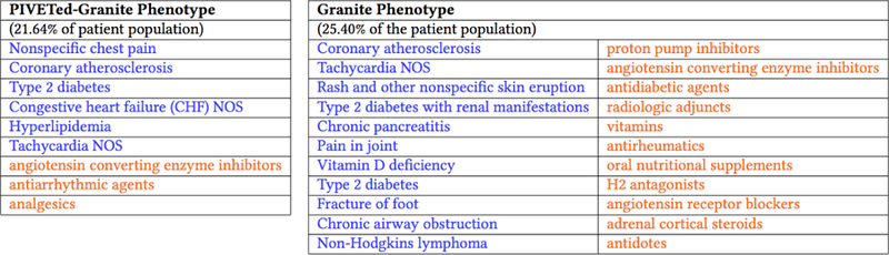
Two phenotypes, one derived using CP-CLIC-one-shot (left) and one using Granite (right) where both methods were initialized with the same factor vetors.

3. Methods and Technical Solutions

Unlike existing constrained tensor decomposition models, CP-CLIC gradually learns constraints about intermode relationships within tensors and refines these constraints using auxiliary information. Automatically discovering the relevant constraints reduces the up-front guidance costs associated with domain experts and guards against overfitting to existing domain knowledge. Moreover, it allows the decomposition to discover the multiway relationships in a data-driven fashion. Furthermore, users can encode their uncertainty in the auxiliary information without necessitating domain expert supervision throughout the entire process. CP-CLIC is formulated to accommodate a large family of objective functions that work in concert with sparsity- and diversity-encouraging constraints to derive meaningful components.

The objective function is formulated as follows. Let $\mathcal{X}$ denote an $I_1\times I_2\times \cdots \times I_N$ tensor and $\mathcal{Z}$ represent a same-sized tensor where each element $z_{\overrightarrow{i}}$ contains the optimal parameters of the observed tensor $x_{\overrightarrow{i}}$. The full objective function of CP-CLIC is as follows:

$$f\left(\mathcal{X}\right)=\min \mathcal{L}\left(\mathcal{Z}|\mathcal{X}\right)$$ (3.1)

$$+{\beta }_1\sum _{n=1}^N\sum _{m=1}^{n-1}\text{Tr}\left({\mathbf{\text{A}}}^{\left(m\right){\rm T}}{\mathbf{\text{M}}}^{\left(m,n\right)}{\mathbf{\text{A}}}^{\left(n\right)}\right)$$ (3.2)

$$+\frac{{\beta }_2}{2}\sum _{n=1}^N\sum _{r=1}^R\sum _{p=1}^r\max \hspace{0.17em}{(0,\frac{{({\mathbf{\text{a}}}_p^{\left(n\right)})}^{{\rm T}}{\mathbf{\text{a}}}_r^{\left(n\right)}}{{\Vert {\mathbf{\text{a}}}_p^{\left(n\right)}\Vert }_2{\Vert {\mathbf{\text{a}}}_r^{\left(n\right)}\Vert }_2}-{\theta }_n)}^2$$ (3.3)

$$+\frac{{\beta }_3}{2}\sum _{n=1}^N\sum _{r=1}^R{\Vert {\mathbf{\text{a}}}_r^{\left(n\right)}\Vert }_2^2$$ (3.4)

$$\begin{gathered} \text{s.t}\hspace{0.17em}\mathcal{Z}=〚\lambda ;{\mathbf{\text{A}}}^{\left(1\right)};\cdots ;{\mathbf{\text{A}}}^{\left(N\right)}〛 \\ \hspace{0.17em}\hspace{0.17em}{\lambda }_r\ge 0,\hspace{0.17em}\hspace{0.17em}\forall r;{\mathbf{\text{A}}}^{\left(n\right)}\in {\left[0,1\right]}^{I_n\times R},{\theta }_n\in \left[0,1\right]\forall n \end{gathered}$$ (3.5)

$${\Vert {\mathbf{\text{a}}}_r^{\left(n\right)}\Vert }_1=1,\hspace{0.17em}\hspace{0.17em}\forall n$$ (3.6)

The parameters $z_{\overrightarrow{i}}$ can be determined by minimizing the negative log-likelihood of the observed $x_{\overrightarrow{i}}$ and model the parameters $z_{\overrightarrow{i}}$ (see Equation 3.1). We augment the Equation 3.1 with constraints to encourage rank-one components that are sparse, diverse, and meaningful.

3.1. Bregman Divergence

While least squares is commonly used to fit the CP decomposition, it is not well-suited for all types of data. A large number of other useful loss functions such as KL divergence, logistic loss, and Itakura-Saito distance may be more appropriate for count data or binomial data. As such, we propose the generalization of the loss, $\mathcal{L}\left(\mathcal{Z}|\mathcal{X}\right)$ in Equation 3.1, in terms of the Bregman divergence. Bregman divergences encompass a broad range of useful loss functions, with common ones listed in Table 1.

Table 1:

Bergman divergence loss functions and gradients where ${\mathbf{\text{A}}}^{\left(-n\right)}\equiv {\mathbf{\text{A}}}^{\left(N\right)}\odot \cdots \odot {\mathbf{\text{A}}}^{\left(n+1\right)}\odot {\mathbf{\text{A}}}^{\left(n-1\right)}\odot \cdots \odot {\mathbf{\text{A}}}^{\left(1\right)}$.

Bregman Divergence	Negative Log-Likelihood	Matricized Gradient $(\text{i,e.,}\frac{\partial \mathcal{L}\left(\mathcal{Z}|\mathcal{X}\right)}{\partial {\mathbf{\text{A}}}^{\left(n\right)}})$
Mean-squared	$\frac{1}{2}{\left(x_{\overrightarrow{i}}-z_{\overrightarrow{i}}\right)}^2$	$\left({\mathbf{\text{Z}}}_{\left(n\right)}-{\mathbf{\text{X}}}_{\left(n\right)}\right){\mathbf{\text{A}}}^{\left(-n\right)}$
Exponential	$x_{\overrightarrow{i}}{z}_{\overrightarrow{i}}-\log z_{\overrightarrow{i}}$	$\left({\mathbf{\text{X}}}_{\left(n\right)}-\mathrm{𝟙}\oslash {\mathbf{\text{Z}}}_{\left(n\right)}\right){\mathbf{\text{A}}}^{\left(-n\right)}$
Poisson	$z_{\overrightarrow{i}}-x_{\overrightarrow{i}}\log z_{\overrightarrow{i}}$	$\left(\mathrm{𝟙}-{\mathbf{\text{X}}}_{\left(n\right)}\oslash {\mathbf{\text{Z}}}_{\left(n\right)}\right){\mathbf{\text{A}}}^{\left(-n\right)}$
Boolean	$\log \left(z_{\overrightarrow{i}}+1\right)-x_{\overrightarrow{i}}\log z_{\overrightarrow{i}}$	$\left(\mathrm{𝟙}\oslash \left({\mathbf{\text{Z}}}_{\left(n\right)}+\mathrm{𝟙}\right)-{\mathbf{\text{X}}}_{\left(n\right)}\oslash {\mathbf{\text{Z}}}_{\left(n\right)}\right){\mathbf{\text{A}}}^{\left(-n\right)}$

3.2. Constraints

Stochastic Constraints

The column stochastic constraints (Equation 3.6) allow each non-zero element to be interpreted as a conditional probability given the component (e.g., phenotype and mode). A high (close to 1) value indicates a strong relationship for this element in the component. Alternatively, a low probability (close to 0) represents a weak relationship.

Cannot-link Constraints

The cannot-link constraints, expressed in Equation 3.2, are motivated by the probabilistic interpretation of the components. During the fitting process, CP-CLIC identifies the elements with low probabilities in each mode in each component (i.e., probabilities less than α) and discourages them from appearing together in the component through the penalty imposed by Equation 3.2. In Equation 3.2, ${\mathbf{\text{M}}}^{\left(m,n\right)}\in {\mathbf{1}}^{I_m\times I_n}$ is a binary cannot-link matrix between modes m and n, defined as follows:

$${\mathbf{\text{M}}}_{jk}^{\left(m,n\right)}=\{\begin{array}{l}1,\hspace{1em}\text{if}\hspace{0.17em}{\mathbf{\text{a}}}_{jr}^{\left(m\right)}<\alpha \hspace{0.17em}\text{and}\hspace{0.17em}{\mathbf{\text{a}}}_{kr}^{\left(n\right)}<\alpha \hspace{0.17em}\text{for}\hspace{0.17em}\text{any}\hspace{0.17em}r\\ 0,\hspace{1em}\text{otherwise}\end{array}$$

The terms in Equation 3.2 are of the form, $a_{jr}^{\left(m\right)}{\mathbf{\text{M}}}_{jk}^{\left(m,n\right)}{a}_{kr}^{\left(n\right)}$, and only contribute to the objective function if the j^th object in mode m and the k^th object in mode n appear in at least one of the R components. This constraint may also encourage sparsity in the number of elements per component since it is penalizing the smaller elements of the factors. We set α to be an exponential loss function of k, the number of non-zeros per factor, and the epoch l. If all elements have equal probability (i.e., the are equally uninformative), they will have probability 1/k. However, we exponentially increase α to 1/k over the epochs in order to be more aggressive as the fit continues.We describe how to refine M^(m,n) in Section 3.4.

Sparsity and Diversity Constraints

We follow Henderson et al. [6] and incorporate Equations 3.3 and 3.4, which are used to encourage diversity of the components through an angular penalty on the vectors within each factor matrix, and to control the size of the λ weights that are fit, respectively. Equation 3.3 calculates the cosine similarity between each pair of factor vectors in a mode and adds to the penalty if the similarity is greater than θ_n. A smaller θ_n encourages factor vectors to be orthogonal to one another whereas a larger θ_n allows for more overlap between factor vectors. To encourage sparse solutions, we project the largest k terms in each factor vector onto an ℓ₁ ball.

$$\begin{array}{l}\overline{\underset{¯}{\mathbf{\text{Algorithm}}\hspace{0.17em}\mathbf{1}\hspace{0.17em}\text{CP-CLIC fitting process}\hspace{1em}\hspace{1em}\hspace{1em}\hspace{1em}\hspace{1em}\hspace{1em}\hspace{1em}\hspace{1em}\hspace{1em}\hspace{1em}\hspace{1em}}}\\ \hspace{0.17em}\hspace{0.17em}\text{1:}\hspace{0.17em}\hspace{0.17em}\text{Randomly}\hspace{0.17em}\text{initialize}\hspace{0.17em}〚\lambda ;{\mathbf{\text{A}}}^{\left(1\right)};{\mathbf{\text{A}}}^{\left(2\right)}\cdots ;{\mathbf{\text{A}}}^{\left(N\right)}〛\\ \hspace{0.17em}\hspace{0.17em}\text{2:}\hspace{0.17em}\hspace{0.17em}{S}_{\text{all}}=\varnothing ;{\mathbf{\text{M}}}^{\left(m,n\right)}=\text{zeros}\left(I_m,I_n\right)\text{for}\hspace{0.17em}\text{each}\hspace{0.17em}m,n\hspace{0.17em}\text{pair}\\ \hspace{0.17em}\hspace{0.17em}\text{3:}\hspace{0.17em}\hspace{0.17em}\mathbf{\text{for}}\hspace{0.17em}l=1:L\hspace{0.17em}\mathbf{\text{do}}\\ \hspace{0.17em}\hspace{0.17em}\text{4:}\hspace{1em}\hspace{0.17em}\hspace{0.17em}\text{Run}\hspace{0.17em}\text{epoch}\hspace{0.17em}\text{of}\hspace{0.17em}\text{SGD}\hspace{0.17em}\text{with}\hspace{0.17em}\text{Adam}\\ \hspace{0.17em}\hspace{0.17em}\text{5:}\hspace{1em}\hspace{0.17em}\hspace{0.17em}\mathbf{\text{for}}\hspace{0.17em}m,n\hspace{0.17em}\text{pairs}\hspace{0.17em}\mathbf{\text{do}}\\ \hspace{0.17em}\hspace{0.17em}\text{6:}\hspace{1em}\hspace{0.17em}\hspace{0.17em}S=\varnothing \\ \hspace{0.17em}\hspace{0.17em}\text{7:}\hspace{1em}\hspace{0.17em}\hspace{0.17em}\mathbf{\text{for}}\hspace{0.17em}\text{r}=1:\text{R}\hspace{0.17em}\mathbf{\text{d}}\text{o}\\ \hspace{0.17em}\hspace{0.17em}\text{8:}\hspace{1em}\hspace{1em}\hspace{0.17em}\hspace{0.17em}\hspace{0.17em}\#\mathtt{\text{Find}}\hspace{1em}\mathtt{\text{low}}\hspace{1em}\mathtt{\text{prob.}}\hspace{1em}\text{elements}\\ \hspace{0.17em}\hspace{0.17em}\text{9:}\hspace{1em}\hspace{1em}\hspace{0.17em}\hspace{0.17em}\hspace{0.17em}{S}_m=\left\{{\mathbf{\text{a}}}_{jr}^{\left(m\right)}<\alpha ,0\le j\le I_m\right\}\\ \text{10:}\hspace{1em}\hspace{1em}\hspace{0.17em}\hspace{0.17em}\hspace{0.17em}{S}_n=\left\{{\mathbf{\text{a}}}_{kr}^{\left(n\right)}<\alpha ,0\le k\le I_n\right\}\\ \text{11:}\hspace{1em}\hspace{1em}\hspace{0.17em}\hspace{0.17em}\hspace{0.17em}\text{\#}\hspace{0.17em}\mathtt{\text{Obtain}}\hspace{1em}\mathtt{\text{all}}\hspace{1em}\mathtt{\text{combos}}\hspace{1em}\mathtt{\text{of}}\hspace{0.17em}{S}_m\hspace{0.17em}\text{and}\hspace{0.17em}{S}_n\\ \text{12:}\hspace{1em}\hspace{1em}\hspace{0.17em}\hspace{0.17em}\hspace{0.17em}S=S\cup \left\{S_m\times S_n\right\}\\ \text{13:}\hspace{1em}\hspace{1em}\mathbf{\text{end}}\hspace{1em}\mathbf{\text{for}}\\ \text{14:}\hspace{1em}\hspace{1em}\text{Send }S\text{ to auxiliary tool}\\ \text{15:}\hspace{1em}\hspace{1em}{S}_{\text{lift}}=\left\{lift(m,n)=\frac{P(m\cap n)}{P(m)P(n)}>1\right\}\\ \text{16:}\hspace{1em}\hspace{1em}{S}_{\text{all}}=S_{\text{all}}\cup (S-S_{\text{lift}})\\ \text{17:}\hspace{1em}\hspace{1em}\text{\#}\mathtt{\text{ Set elements in }}S\text{ equal to 1}\\ \text{18:}\hspace{1em}\hspace{1em}{\mathbf{\text{M}}}_{jk}^{(m,n)}=\{\mathrm{𝟙}:j,k\in S_{\text{all}}\}\\ \text{19:}\hspace{1em}\hspace{1em}\mathbf{\text{end}}\hspace{1em}\mathbf{\text{for}}\\ \text{20:}\hspace{1em}\hspace{1em}\text{Check convergence}\\ \text{21:}\hspace{0.17em}\hspace{0.17em}\mathbf{\text{end}}\hspace{1em}\mathbf{\text{for}}\\ \underset{\_}{\text{22:}\hspace{0.17em}\hspace{0.17em}\mathbf{\text{return}}\hspace{0.17em}\hspace{0.17em}〚\lambda ;{\mathbf{\text{A}}}^{\left(1\right)};{\mathbf{\text{A}}}^{\left(2\right)}\cdots ;{\mathbf{\text{A}}}^{\left(N\right)}〛}\end{array}$$

3.3. Minimizing the objective function

We minimize the objective function using Stochastic Gradient Descent (SGD) with Adam [18]. We follow the work on Generalized CP Decomposition presented by Kolda et al for the implementation [19]. Using SGD to minimize a CP gradient is equivalent to a sparse implementation of CP decomposition where a subset of data points are taken to be the non-zero entries. We use the work of Acar et al. [20] to implement operations on sparse tensors. After each epoch, CP-CLIC finds the low probability elements in each component and updates the cannot-link matrix, M^(m,n) (outlined in Algorithm 1 and Figure 1).

For the gradient of Equation 3.1, we give several examples of widely used loss functions in Table 1. We refer the reader to [6] for the gradients for Equations 3.3 and 3.4. For Equation 3.2, the derivative with respect to the factor matrix A^(m) is:

$$\frac{\partial \text{Tr}\left({\mathbf{\text{A}}}^{\left(m\right){\rm T}}{\mathbf{\text{M}}}^{\left(m,n\right)}{\mathbf{\text{A}}}^{\left(n\right)}\right))}{\partial {\mathbf{\text{A}}}^{\left(m\right)}}={\mathbf{\text{M}}}^{\left(m,n\right)}{\mathbf{\text{A}}}^{\left(n\right)}$$ (3.7)

$$\frac{\partial \text{Tr}\left({\mathbf{\text{A}}}^{\left(m\right){\rm T}}{\mathbf{\text{M}}}^{\left(m,n\right)}{\mathbf{\text{A}}}^{\left(n\right)}\right))}{\partial {\mathbf{\text{A}}}^{\left(n\right)}}={\mathbf{\text{M}}}^{\left(m,n\right){\rm T}}{\mathbf{\text{A}}}^{\left(m\right)}$$ (3.8)

3.4. Incorporating insights from auxiliary information

One possible drawback of building the cannot-link matrix in an unsupervised manner is that it is possible for two elements to have low probability in a component but actually have a relationship in the domain in question. To mitigate the chance of this occurrence, CP-CLIC uses auxiliary information to accept or reject the cannot-link constraints. Figure 1 gives a stylized view of how CP-CLIC incorporates auxiliary information. Algorithm 1 specifies how the cannot-link penalty matrix is built through the fitting process. After each epoch, CP-CLIC extracts the intermode pairs that have a probability below a threshold.² Then, for each pair, if there is insufficient evidence that the relationship exists according to auxiliary information, CP-CLIC puts a 1 in the cannot-link matrix for that pair. The updated cannot-link penalty matrix is then incorporated into the next epoch of the fitting process.

In practice, auxiliary information could come in many forms (e.g., online forums). In Section 4 we show how to incorporate information from a corpus of medical journals. It may be possible to use the auxiliary information to build a cannot-link matrix and hard-code the constraints into M^(m,n) from the beginning of the fit instead of gradually building the cannot-link matrix as the fit progresses. This approach, which we refer to as CP-CLIC-1-Shot, may be appropriate in situations where the user has confidence in the veracity of the auxiliary information. In other applications, however, the user might not have as much confidence in the auxiliary information. Using CP-CLIC-1-Shot in these applications may introduce noise into the decomposition and degrade the quality of the fit. Thus, gradually building the constraints in CP-CLIC may be more robust to introducing noise in M^(m,n) matrix.

4. Empirical Evaluation

4.1. Simulated Data

First, we demonstrate that the CP-CLIC framework is general enough to be used with different loss functions. We evaluate CP-CLIC’s performance against three types of synthetic tensors, where elements are drawn from a Poisson, Normal, or Exponential distribution, and we compare the performance to CP-ALS [1], a popular tensor decomposition method that uses mean-squared loss between the observed tensor and the fit tensor as the objective function. Specifically, we simulate third-order tensors of size 80×40×40 with a rank of 5 (R = 5). For each vector in the factor matrix A⁽ⁿ⁾, we sample non-zero element indices according to a chosen sparsity pattern (20, 12, and 12 non-zero elements in mode 1, 2, and 3, respectively) and then randomly sample along the simplex for the non-zero indices, rejecting vectors that are too similar to those already generated (i.e., their normalized cosine angle is greater than θ_n). We draw the model parameters z_ijk from a uniform distribution. Finally, each tensor element x_ijk is sampled from a Poisson, Normal, or Exponential distribution with the parameter set to z_ijk. For each tensor type, we simulated 40 tensors and calculated the factor match score with the known vectors where a value of 1 representing a perfect match [11].

Table 2 shows the factor match scores for fits with and without β₁. In all cases, CP-CLIC improves the quality of the fit and makes the biggest impact in the Exponential case. Thus, for common data types, CP-CLIC can recover the original factors. CP-ALS’s poor performance on the tensors containing count and exponential data underscores the importance of choosing a loss function that aligns with how the data are generated. Computational phenotyping methods that use the same loss function as CP-ALS but on tensors of count data, which we use as baselines in the next section, may sacrifice quality of fit.

Table 2:

Factor match scores between fitted factor vectors and known factor vectors generated using Poisson, Normal, and Exponential distributions.

Data	Mode	CP-ALS	CP-CLIC
			β1 = 0	β1 = 0.01
Real	1	0.940	0.988	0.991
	2	0.921	0.994	0.997
	3	0.939	0.995	0.997
Count	1	0.555	0.934	0.977
	2	0.629	0.946	0.958
	3	0.620	0.946	0.967
Exponential	1	0.121	0.883	0.945
	2	0.167	0.894	0.967
	3	0.199	0.902	0.963

4.2. CP-CLIC in Computational Phenotyping

Dataset Description

We constructed a tensor from a set of de-identified EHRs from the Vanderbilt University Medical Center (VUMC) in Nashville, TN, a medical system that serves a wide area of the south-eastern United States through a collection of hospitals, clinics, and other healthcare facilities. To build the tensor, we counted the medication and diagnosis interactions that occurred two years before the date of the patient’s last interaction with the medical center. The diagnosis codes are from the International Classification of Diseases - version 9 (ICD-9) system, which captures detailed information for billing purposes. We use Phenome-Wide Association Study (PheWAS) coding to aggregate the diagnosis codes into broader categories [21]. We group the medication codes into more general categories using the Medical Subject Headings (MeSH) pharmacological terms provided by the US National Library of Medicine’s RxClass RESTful API.³ Aggregating the codes allows for larger trends to emerge in the components and makes it possible for future use in various types of association investigations, such as genomic studies. These groupings resulted in a tensor with the following dimensions: 1622 patients (mode 1) by 1325 diagnoses (mode 2) by 148 medications (mode 3). Within the set of patients, domain experts previously identified 304 as resistant hypertension case patients and 399 control patients.

Since the EHR tensor contains counts, we use KL-divergence for $\mathcal{L}\left(\mathcal{Z}|\mathcal{X}\right)$. For feasibility and numerical stability, we augment the R components with a rank-one bias tensor, a strictly positive rank-one tensor. We refer the reader to [17] for details. Parameter values for CP-CLIC variants and Granite were chosen using a grid search and the KL-divergence as a measure of performance. The grid search was over the following ranges: R = [20, 50], β₁ = [.01, 100], β₂ = [0, 10], β₃ = [.0001, 10], θ_n = [.15, 1], for n = {1, 2}, θ₁ = 1.

Incorporating auxiliary information in practice

We use a tool called Phenotype Instance Verification and Evaluation Tool (PIVET) to evaluate the cannot-link constraints [22]. When phenotypes have been derived through automatic machine learning methods, it is necessary to verify that they map to clinically relevant concepts. This task is usually performed by domain experts who volunteer their time to annotate the clinical validity of sets of phenotypes. The annotation task can sometimes lead to ambiguity and experts may disagree about the clinical relevance of a set of phenotypic characteristics [22]. PIVET was developed to aid in the phenotype verification task. PIVET analyzes an openly available medical journal article corpus to build evidence sets for the clinical relevance of provided phenotypes. The analysis is built on the concept of lift [23], where the lift between objects m and n is defined as $\text{lift}\left(m,n\right)=\frac{P\left(m\cap n\right)}{P\left(m\right)P\left(n\right)}$. A lift value of greater than one suggests that the objects co-occur often. We use lift as calculated by PIVET to prune lists of possible cannot-link pairs of diagnoses and medications.

Computational Phenotyping Results

We evaluate CP-CLIC quantitatively and qualitatively to determine their utility to clinicians. First, we compare features of decompositions of three variations of CP-CLIC (i.e., CP-CLIC, CP-CLIC-1-Shot, and CP-CLIC without PIVET) with four baselines: Granite (fit using SGD), CP-APR, Rubik [8], and DDP, which refers to the model presented by Kim et al [14].⁴ Second, we evaluate each method’s ability to discriminate between case and control patients. Third, we qualitatively analyze a subset of phenotypes extracted using CP-CLIC-1-Shot and Granite in a case study. We show results for the fits resulting from the parameter values of R = 30, θ₁ = 1, θ₂ = .45, θ₃ = .75, β₁ = .01, β₂ = {0, 10},⁵ β₃ = .001, and a burn-in of 5 epochs.

Table 3 shows the average cosine similarity between the factor vectors in each mode and the average number of non-zeros per mode. CP-CLIC finds diverse factors with respect to the tensor. For this particular tensor, experiments showed the diversity penalty could be strict for the diagnosis mode because there were many diagnoses (θ₂ = .45), but the relatively few medications benefited from a more lax diversity penalty (θ₃ = .75). All CP-CLIC variations produce diagnosis and medication modes that are comparably diverse to those derived through GraniteSGD. Table 3 shows the diagnosis mode is quite diverse and there is more overlap in the medication mode.⁶ Rubik, which has orthogonality constraints, had comparable diversity to Granite and CP-CLIC in modes 2 and 3, but had a much more diverse patient mode (mode 1), which may stem from the fact that there were so few patients in each component. CP-CLIC’s patient vectors have more in common with each other (i.e., higher cosine similarity scores) indicating that similar groups of patients belong to the same phenotypes overall.

Table 3:

Mean cosine similarity and average number of non-zeros the factor vectors in each mode (✓ means β₂ > 0, 0 ≤ θ_n ≤ 1 to encourage diversity).

Method	Diversity Penalty	Cosine Similarity			Number of Non-zeros
		Mode 1	Mode 2	Mode 3	Mode 1	Mode 2	Mode 3
CP-APR		0.00 (0.00)	0.22 (0.00)	0.18 (0.00)	22.62 (1.00)	42.21 (1.14)	21.86 (0.23)
Rubik		0.02 (0.01)	0.05 (0.01)	0.14 (0.01)	7.48 (2.73)	26.65 (4.01)	15.19 (2.16)
DDP		0.03 (0.00)	0.07 (0.00)	0.11 (0.00)	77.79 (5.28)	44.01 (1.99)	17.01 (0.53)
GraniteSGD		0.31 (0.01)	0.06 (0.01)	0.13 (0.01)	73.26 (1.03)	13.07 (0.65)	10.85 (0.54)
GraniteSGD	✓	0.18 (0.01)	0.02 (0.01)	0.12 (0.01)	70.45 (1.69)	18.21 (1.06)	12.31 (0.31)
CP-CLIC- 1-shot		0.19 (0.02)	0.04 (0.02)	0.08 (0.02)	57.87 (3.67)	10.14 (0.28)	8.91 (0.12)
CP-CLIC- 1-Shot	✓	0.17 (0.02)	0.01 (0.02)	0.09 (0.02)	64.75 (5.73)	9.55 (0.21)	8.61 (0.21)
CP-CLIC, no pruning		0.31 (0.02)	0.06 (0.02)	0.12 (0.02)	71.63 (1.68)	13.53 (0.70)	11.28 (0.39)
CP-CLIC, no pruning	✓	0.24 (0.02)	0.03 (0.02)	0.14 (0.02)	72.29 (1.85)	16.65 (1.04)	11.79 (0.31)
CP-CLIC		0.32 (0.01)	0.05 (0.01)	0.11 (0.01)	66.83 (0.91)	11.87 (0.93)	9.51 (0.55)
CP-CLIC	✓	0.28 (0.02)	0.03 (0.02)	0.14 (0.02)	69.09 (0.99)	16.73 (0.49)	10.37 (0.37)

In terms of sparsity (Table 3), the unconstrained method CP-APR has on average the most non-zero elements in the factor vectors of mode 3 (medication) with 21.86 elements. In mode 2 (diagnosis), DDP has the largest number non-zero elements in each factor vector with an average of 44.01 elements. Overall, in the diagnosis and medication modes, CP-CLIC-1-Shot model has sparsest factors with an average of 9.55 and 8.61 nonzero elements per factor vector, respectively, followed by CP-CLIC. Sparse components are generally easier for clinicians to interpret and utilize.

Additionally, we evaluated the discriminative capabilities of CP-CLIC on a prediction task where the patient factor matrix served as the feature matrix. We compared the performance of CP-CLIC, CP-CLIC-1-shot, Granite, Rubik, and DDP using logistic regression to predict which patients were resistant hypertension cases. The model was run with 5-fold cross validation with 80–20 train-test splits, and the optimal LASSO parameter for the model was learned using 10-fold cross-validation on a holdout set. Table 4 shows the area under the receiver operator characteristic curve (AUC) for the task. The patient factor matrix derived using CP-CLIC-1-shot resulted in the most discriminative model. Both Rubik and DDP performed quite poorly, and this may be related to the diverse patient mode (Table 3).

Table 4:

AUC for predicting resistant hypertension case patients.

Method	AUC (st. dev.)
Rubik	0.5398 (0.03)
DDP	0.6466 (0.12)
Granite	0.6545 (0.08)
CP-CLIC-1-shot	0.7015 (0.10)
CP-CLIC	0.6755 (0.09)

To evaluate the effect of the cannot-link matrix M on the decomposition process we initialized CP-CLIC-1-shot and Granite fits with the same factors and then examined the differences between the fitted factors. For the sake of brevity, Figure 2 shows only one phenotype from each method initialized from the same factors. Two clinicians reviewed the two phenotypes in Figure 2 and concluded the CP-CLIC-1-Shot phenotype aligns with their definition of a typical cardiovascular patient. While a patient with the CP-CLIC-1-Shot phenotype may have the same comorbidities as the Granite phenotype, the Granite phenotype also contains items that seem more incidental (e.g. cardiovascular issues with Lymphoma). Thus, the focused and succinct CP-CLIC-1-Shot phenotype has potential for more general use in future clinical research.

5. Signiftcance and Impact

This research shows that adding guidance, in the form of constraints, to tensor decompositions can improve the quality of the derived components in terms of interpretability, sparsity, and diversity. However, obtaining informative constraints can be expensive in regard to time and effort required by domain experts. This work shows that features of the CP decomposition process can be utilized to discover constraints through the learning method. The framework, CP-CLIC, gradually uncovers between-mode cannot-link constraints and then validates the constraints using domain expertise in the form of auxiliary information. CP-CLIC is a flexible framework in that it 1) works on all or a subset of modes of the tensor and 2) is well-suited for many different types of data. In situations where the quality of the auxiliary information is high, it may be appropriate to forgo the gradual discovery of cannot-link constraints and supply the dense cannot-link matrix at the beginning of the learning process (CP-CLIC-1-Shot). We show that in both simulated and computational phenotyping experiments, gradually discovering the constraints can improve the quality of the results.

References

- [1].Kolda TG and Bader BW. Tensor decompositions and applications. SIAM Rev, 51(3):455–500, 2009. [Google Scholar]
- [2].Harshman RA. Foundations of the PARAFAC procedure: Models and conditions for an “explanatory” multimodal factor analysis. UCLA Working Papers in Phonetics, 16:1–84, 1970. [Google Scholar]
- [3].Pathak J, Kho AN, and Denny JC. Electronic health records-driven phenotyping: challenges, recent advances, and perspectives. J Am Med Inf Assoc (JAMIA), 20(e2):e206–11, 2013. [DOI] [PMC free article] [PubMed] [Google Scholar]
- [4].Richesson RL, Sun J, Pathak J, Kho AN, and Denny JC. Clinical phenotyping in selected national networks: demonstrating the need for high-throughput, portable, and computational methods. AI in Med, 71:57–61, 2016. [DOI] [PMC free article] [PubMed] [Google Scholar]
- [5].Yadav P, Steinbach M, Kumar V, and Simon G. Mining electronic health records (ehrs): a survey. ACM Computing Surveys (CSUR), 50(6):85, 2018. [Google Scholar]
- [6].Henderson J, Ho JC, Kho AN, et al. Granite: Diversified, sparse tensor factorization for electronic health record-based phenotyping. In Fifth IEEE Int Conf on Healthc Inform, volume 2017, pages 214–223. IEEE, 2017. [Google Scholar]
- [7].Carroll JD, Pruzansky S, and Kruskal JB. Candelinc: A general approach to multidimensional analysis of many-way arrays with linear constraints on parameters. Psychometrika, 45(1):3–24, March 1980. ISSN 1860–0980. [Google Scholar]
- [8].Wang Y, Chen R, Ghosh J, et al. Rubik: Knowledge guided tensor factorization and completion for health data analytics. In Proc of ACM SIGKDD Int Conf on Know Disc and Data Min, pages 1265– 1274, 2015. [DOI] [PMC free article] [PubMed] [Google Scholar]
- [9].Davidson I, Gilpin S, Carmichael O, and Walker P. Network discovery via constrained tensor analysis of fMRI data. In Proc of 19th ACM SIGKDD Int Conf on Knowl Discov Data Min, pages 194–202, 2013. [Google Scholar]
- [10].Narita A, Hayashi K, Tomioka R, and Kashima H. Tensor factorization using auxiliary information. Data Min and Know Disc, 25(2):298– 324, September 2012. [Google Scholar]
- [11].Chi EC and Kolda TG. On tensors, sparsity, and nonnegative factorizations. SIAM J Matrix Anal Appl, 33(4):1272–1299, 2012. [Google Scholar]
- [12].Bregman LM. The relaxation method of finding the common point of convex sets and its application to the solution of problems in convex programming. USSR Comput Math and Math Phys, 7(3):200–217, 1967. [Google Scholar]
- [13].Peng W. Constrained nonnegative tensor factorization for clustering. In Proc. of 2010 Ninth Int. Conf. on Mach. Learn. and App., pages 954–957, December 2010. [Google Scholar]
- [14].Kim Y, El-Kareh R, Sun J, Yu H, and Jiang X. Discriminative and distinct phenotyping by constrained tensor factorization. Sci rep, 7(1):1114, 2017. [DOI] [PMC free article] [PubMed] [Google Scholar]
- [15].Luo Y, Wang F, and Szolovits P. Tensor factorization toward precision medicine. Briefings in bioinformatics, 18(3):511–514, 2016. [DOI] [PMC free article] [PubMed] [Google Scholar]
- [16].Ho JC, Ghosh J, and Sun J. Marble: High-throughput phenotyping from electronic health records via sparse nonnegative tensor factorization. In Proc of ACM Int Conf on Knowl Discov Data Min, pages 115–124, 2014. [Google Scholar]
- [17].Ho JC, Ghosh J, Steinhubl SR, et al. Lime-stone: High-throughput candidate phenotype generation via tensor factorization. J Biomed Inf, 52: 199–211, December 2014. [DOI] [PMC free article] [PubMed] [Google Scholar]
- [18].Kingma DP and Ba J. Adam: A method for stochastic optimization. In 3rd Int Conf for Learn Rep, 2015. [Google Scholar]
- [19].Hong D, Kolda TG, and Anderson-Bergman C. Stochastic gradient for generalized CP tensor decomposition (preliminary results) Presentation by T. G. Kolda at Autumn School: Optimization in Machine Learning and Data Science, Trier University, Trier, Germany, August 2017. [Google Scholar]
- [20].Acar E, Dunlavy DM, Kolda TG, and Mrup M. Scalable tensor factorizations for incomplete data. Chemometr Intell Lab Syst, 106(1):41 – 56, 2011. [Google Scholar]
- [21].Denny JC, Bastarache L, Ritchie MD, et al. Systematic comparison of phenome-wide association study of electronic medical record data and genome-wide association study data. Nat Biotechnol, 31(12):1102–1111, November 2013. [DOI] [PMC free article] [PubMed] [Google Scholar]
- [22].Henderson J, Ke J, Ho CJ, Ghosh J, and Wallace CB. Phenotype instance verification and evaluation tool (PIVET): A scaled phenotype evidence generation framework using web-based medical literature. J Med Internet Res, 20(5):e164, May 2018. [DOI] [PMC free article] [PubMed] [Google Scholar]
- [23].Brin S, Motwani R, Ullman JD, and Tsur S. Dynamic itemset counting and implication rules for market basket data. In Proc ACM SIGMOD Int Conf Manag Data, 1997. [Google Scholar]
- [24].Choi Y, Chiu CY-I, and Sontag D. Learning low-dimensional representations of medical concepts. AMIA Jt Summits Transl Sci Proc, 2016:41. [PMC free article] [PubMed] [Google Scholar]