Improving length of stay prediction using a hidden Markov model

Abstract

Estimating length of stay of intensive care unit patients is crucial to reducing health care costs. This can help physicians intervene at the right time to prevent adverse outcomes for the patients. Moreover, resource allocation can be optimized to ensure appropriate hospital staff levels. Yet the length of stay prediction is very hard, as physicians can only accurately estimate half of their patient population. As electronic health records have become more prevalent, researchers can harness the power of machine learning to accurately predict the length of stay. We propose a hidden Markov model-based framework to predict the length of stay using some of patients’ physiological measurements during the first 48 hours of their admission to the intensive care unit. We show that this model can succinctly capture temporal patient representations. We demonstrate the potential of our framework on real ICU data in consistently outperforming most of the existing baselines.

Introduction

A firm grasp of the expected length of stay of an intensive care unit (ICU) patient is crucial for all players involved in the health care industry. Given the high equipment costs and the large percentage of medical resources used by ICU patients, having an accurate estimate of when each resource is likely to become available due to discharge or alternative hospital stays, can lead to considerable optimizations for resource management¹. Not only does this lead to cost reductions for the hospital, but the patient as well. More importantly, once high-risk patients are identified, hospital staff can assign highly trained and valuable specialists to specifically cater to those patients’ needs. An accurate length of stay estimate can also help physicians intervene in a more timely manner and with better care plans. This can lead to a rise in care receivers satisfaction, ultimately resulting in a higher reputation and credibility for the hospital^1–3. Yet predicting length of stay within an acceptable margin is difficult, as attending physicians fail to accurately predict half of their cases¹. Therefore, there is a great opportunity for machine learning methods to improve the length of stay estimate.

A number of machine learning researchers have attempted to estimate the length of stay. Maharlou et al.³, propose a hybrid neuro-fuzzy method using decision trees and expert knowledge translated into logic rules, with MLP regression neural networks, for predicting length of stay of cardiac surgery patients in ICU. Perez et al.² used hospital data gathered in Columbia hospitals to develop different Markov models for each of the six primary reason for admission to ICU. The learned model was reported to be helpful to the patient relatives and healthcare professionals. Recent works have proposed the use of classification models by converting length of stay into a binary or multi-class problem. Harutyunyan et al.⁴, introduced a recurrent neural network framework to predict the length of stay of patients as one of the possible ten buckets. Using the same dataset, Gentimis et al.⁵, applied a neural network model to classify patients into long staying patients and short staying patients and showed that neural network approaches do much better than rule based and linear models. While the results have been promising, there are several limitations in the existing models including the restriction to a multi-label classification problem or failure to leverage all of the patient’s measurements for improved accuracy.

With the adoption of electronic health records (EHRs), a majority of an ICU patient’s physiologic measurements are recorded in some form of structured data. The regular recording of vital signs indicate that these measures are deemed as important indicators of patients’ status by the medical community. However, as human evaluators, physicians might not be able to fully and accurately capture the history of changes of all measures and their complex interactions. We believe that modeling the temporal dynamics of each patient can be used to more accurately estimate the length of stay compared to the standard feature representation. Moreover, we posit that an accurate prediction of the patient’s length of stay can be performed using just 48-hours of their physiological time series after their admission to the ICU. Unlike several recent approaches^{4, 5}, we predict the exact length of stay of patients. Although this is more challenging, an estimate of the exact length of stay is substantially more valuable to health care staff, in terms of more accurate planning and allocation of limited resources.

We propose the use of the hidden Markov model (HMM) to track multiple physiologic measurements and their interactions over time and succinctly summarize these trends in a sequence of states elegantly. To accurately learn the new patient representation, we introduce the overlapping time window and ICU type aggregation technique to achieve robust and stable parameter learning of the HMM model. We demonstrate our model’s improved predictive performance on a publicly available dataset of 4000 ICU patients. Our model not only achieves more accurate estimates, but can still maintain similar model interpretability.

Method

We first provide an overview of the problem setup and then describe the general framework for our model as well as the baseline models.

Dataset. We use the Physionet 2012 challenge dataset⁶, which contains 4000 ICU patients and their physiological measurements during the first 48 hours after an ICU admission. This dataset has been chosen because it is publicly available, has been preprocessed and thus is readily accessible for replication. The patients are admitted to four different ICUs: Coronary Care Unit (Type 1); Cardiac Surgery Recovery Unit (Type 2); Medical ICU (Type 3); and Surgical ICU (Type 4). The dataset contains general descriptors including age and gender as well as 37 different physiological measurements. For the purpose of our study, we focus on the seven most commonly available measurements: non-invasive diastolic arterial blood pressure, temperature, heart rate, Glasgow Coma Score, serum glucose, white blood cell count and urine output. Based on previous work for this dataset and medical knowledge on ICU patients, the urine output was aggregated up to each time point in the patients^{7, 8}. We also use age and gender for clustering and missing value imputation for the features. Table 1 summarizes the observation frequencies and percentage of missing values for these seven variables.

Table 1:

Summary statistics of the observation frequencies and percentage of missing values per patient

Feature	Avg. update frequency (minutes)	Average # of observations	% of missing values
Glasgow Coma Scale	1039.85	13.26	1.6
Temperature	223.30	16.13	1.6
Heart Rate	63.29	46.48	1.6
White Blood Cell Count	1023.42	2.63	1.8
Serum Glucose	968.04	2.72	2.8
Urine output	113.54	28.65	2.9
NIDiasABP	112.21	21.73	12.7

HMM model. The Hidden Markov Model (HMM) assumes an underlying Markov process with unobserved (hidden) states (denoted as Z_t) that generates the output. HMMs have been used to analyze hospital infection data⁹, perform gait phase detection¹⁰, and mine adverse drug reactions¹¹. One computational benefit of HMMs (compared to deep learning models) is the independence assumption where given only previous hidden state (Z_t−1), the current (hidden) state (Z_t) is independent of the other previous states (Z₁, · · ·, Z_t−2). Thus, the computation involved in learning the state transition matrix (T), the output probability distribution (p(x_t|Z_t), and the initial transition probabilities (π) is simplified. While no closed form solution exists, the Expectation-Maximization algorithm is typically used to estimate these parameters for a specified number of hidden states (S). Moreover, for continuous measurements, a Gaussian HMM can be used where the output probability distribution is a multivariate Gaussian distribution.

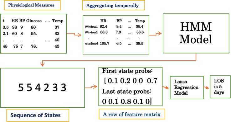
We propose a new feature representation based on the HMM model that can capture the temporal sequences and provide better prediction of the length of stay. Using a specified time resolution (e.g, 8 hours), a summary statistic for each feature (e.g, average, most recent, maximum, etc.) is chosen based on the time window (see Figure 2). A Gaussian HMM is then learned, which later will generate a series of states for each patient with its length corresponding to the number of time windows. The probabilities of the states for the first time window and last time window are used to form a new feature matrix. We hypothesized that HMM will be able to capture the latent underlying states of different patients better than the raw time series features. First and last state were tried out with the intuitive rationale that patients’ beginning and end states can better explain the variance in their length of stay^a. This feature matrix is then used as the input to a regression model to estimate the length of stay. A pictorial description of the steps involved in an HMM model with five states and time resolution of every eight hours for a specific patient is shown in Figure 1.

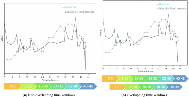
Figure 2:

Example of time windows with time resolution = 8 hours for a given patient in the dataset

Figure 1:

Steps involved in the prediction of length of stay of a given patient using HMM model with 5 states, and time resolution = 8 hours

Given the relatively small sample size, we also introduce preprocessing steps and aggregation techniques to achieve robustness, and improve learning of the parameters of the HMM model. Instead of mutually exclusive (non-overlapping) time windows, we propose the use of overlapping time windows to learn better state transition probabilities. Additional time frames are used that overlap with exactly half of the previous and next time windows. Thus, the time resolution can be chosen such that each time window is likely to have at least one new observation. Moreover, it can smooth over any sensitivity to the specified time resolution. A diagram of non-overlapping and overlapping scheme for a single patient in the dataset is shown in Figure 2 for a time resolution of 8 hours.

It is well-known that there is a marked heterogeneity between different ICUs based on the patient distributions, severity of illness, and durations of admission¹². Yet, learning an individualized HMM model for each ICU may not be feasible due to insufficient samples. For example, in the PhysioNet dataset, the Medical ICU had 1357 patients while Coronary ICU only had 527 patients. Thus, instead of training a single HMM model for patients of all ice types, we propose learning a different model for patients of each group of similar ICU units put together. This way, the learned parameters will have more samples and can guard against overfitting.

Experiment Design

The Physionet dataset was split into an 80% training and 20% testing. To ensure approximately equivalent length of stay distributions, the patients were binned based on their length of stay according to the intervals suggested in a previous work⁴. As a result, there are similar distributions of long-staying and short-staying patients in both training and test datasets. After the split, each feature was normalized to have zero mean and unit standard deviation on the training set, with the same normalization process applied to the test dataset. We also observed that the length of stay in days, as provided in the dataset, led to numerical imprecision in the HMM model. Thus, we converted the patients’ length of stay to hours to guard against numerical instability^b. We also considered only using the first 12 hours or the first 24 hour or the second 24 hour of data. The Root Mean Square Error (RMSE) for all these cases was lower than using all the 48 hours, probably due to the low frequency of updates for measurements, that resulted in insufficient data for the model to be able to learn a meaningful model.

Baseline Models. The predictive performance of our HMM model was evaluated against six common regression models: LASSO regression, ridge regression, Poisson regression, binomial regression, support vector regression (SVR) and only using SAPS-II scores as linear regression features. For these models, the feature matrix consists of summary statistics for each of the seven measurements noted in Table 1. The average, minimum, maximum, first, and last measurements were computed to yield a total of 35 features. We performed correlation analysis of the 35 features using the Pearson correlation coefficient and found some correlated features. Thus, we explored the application of PCA on the feature matrix to reduce redundant features and remove noise. However, in most runs, the number of PCA components needed to capture 95% of the variance was the same as the original features. Hyperparameter tuning for LASSO and ridge were performed using cross-validation of the training data.

HMM Model. We performed several experiments to identify the best configurations with respect to the (1) number of states (S); (2) overlapping or non-overlapping time windows; (3) aggregation of ICU types; (4) the summary measure for each time window (average or last) and (5) selection of timewindows probabilities to include in the final linear model. While there are two other parameters for our model, covariance structure and time resolution, they were chosen based on preliminary experiments. Using the diagonal covariance for the features, we found the HMM model performed better and the learned parameters were more stable. This is consistent with our exploratory analysis, as the selected features had little correlation and thus would not benefit from the more complex spherical covariance structure. Also, we chose the time resolution to match the availability of physiological measures while also minimizing the length of the sequence. We explored using 4, 6, and 8 hours as the time resolution, but found that 8 hours provided good predictive power and stable parameters. Thus, there were either 6 or 11 time frames for non-overlapping and overlapping time windows. We performed multiple experiments using only probabilities of the first time point, both first and last time point and all time points. Using both first and last time point probabilities gave the best results in terms of lowest average and median RMSE, and lowest RMSE variance across 300 runs. Basing our analysis on the same critera, we found that using last available measurement in an interval is better than using average of measurements.

For the purpose of this paper, we use an existing, open-source Python package

hmmlearn

^c to train our HMM model. Grid search was performed for the various parameters across five random splits of the training dataset. The best setting was chosen based on three different criteria. In addition to the lowest value for the cost function associated with the HMM optimization problem, we assessed the parameter value based on the LOS variance across all possible start and end state pairs (greater is better), and variance within each possible start and end state pairs (lower means the patients in that group were more similar).

For training the Gaussian HMM, a number of parameters are set randomly including the initial prior probability of each state, initial transition matrix, mean and precision of the Normal prior distribution, tolerance, and number of iterations. To mitigate the impact of the random initialization, we initialized multiple instances of the HMM model for a given split of data, and observed that the transition matrix and the prior vector do not change significantly over different parameter initializations (they only change in the order of 0.000001). Therefore, the number of iterations of parameter initializations for the HMM model was set to five.

Missing value imputation. Our dataset included many missing values. If a patient had no measurement for any of the seven features, the patient was not included in the experiment. For the baseline feature matrix, missing values were imputed with the mean of that feature across all time points, later the feature matrix was normalized^d. A slightly different approach was taken for the input to our HMM model. If the patient is missing a value for the very first time point for any given feature, the value of the first time point is imputed based on its five nearest neighbors (based on other patients available value). The value of k (k = 5) in the k-nearest neighbor algorithm was chosen as it yielded the lowest mean squared error based on the validation set. Since the first time point for every patient will be present, we used a push forward method to impute any other missing values.

Results

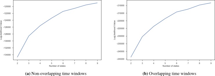
Number of States. A grid search was performed between 2 and 10 to find the optimal number of states while fixing the other free parameters of the model. Figure 3 shows the likelihood value as a function of the number of states, with higher value indicating a better “fit” to the observations. We observe a plateau in the log-likelihood for both the overlapping and the non-overlapping time windows around 8. However, the log likelihood was not the only criteria that we evaluated.

Figure 3:

Value of likelihood function vs number of states

The other criteria we used was to analyze the variance in the LOS of patients across the different start-end state pairs and within each start-end state pairs. The idea is that if there is a high variance across the average or median LOS in the start-end state pairs, this indicates that pairs have well captured the difference of short staying and long staying patients. Similarly, if the average variance of the LOS within each start-end state pair was small, the patients in the pair were homogeneous and may yield good predictors. Figure 4 shows an example of the plot for the overlapping time windows. We analyzed the variance of the median (Figure 4a) and mean LOS (Figure 4b) of the patients across the start-end state groups, and found that it reached a peak around 8 and 9. Moreover, the average variance within each start-end-pair (Figure 4c) was lower for 8 and 9. In conjunction with the loss function, this suggests that S = 8 is the optimal number of states for this dataset.

Figure 4:

Variance of length of stay (LOS) of patients based on the start-end state groups for varying number of states

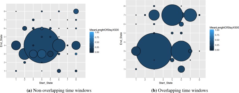
Overlapping Time Windows. We analyzed the impact of using overlapping time windows to train our HMM model. Figure 5 shows the mean length of stay of the patients denoted by color and the number of patients that fall into that group shown using radius of the circle. In overlapping case, we observe not only a more uniform distribution of the patients into the different start-end state pairs but also a larger variance in the mean length of stay. Thus, overlapping time windows can be more advantageous in terms of improving the predictive power.

Figure 5:

Distribution of patients into possible start-end state pairs with time resolution = 8 and S = 8 in overlapping and non overlapping cases

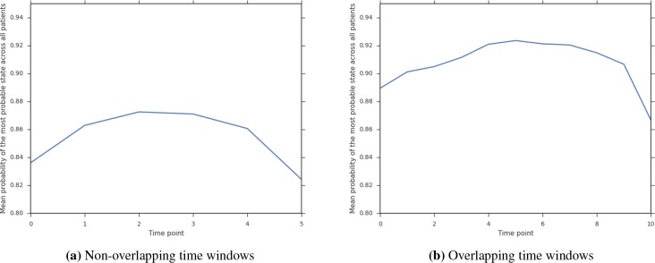
Overlapping windows also provide more certainty about the chosen states for each patient. Given the larger number of measurements per patient (6 vs 11), the HMM model can better estimate a patient’s sequence of states. Figure 6 shows the mean probability of the most probable state at that time point. For overlapping time windows, we observe that the model is more certain about the state for each patient across all the time frames (shown by higher probability).

Figure 6:

Certainty of chosen state with time resolution = 8 and S = 8 overlapping and non overlapping schemes

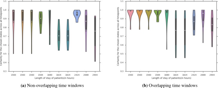
We further analyzed this effect on the patients who end up staying in the ICU for a long time, which even physicians struggle to predict¹. Figure 7 shows a violin plot based on the distribution of the probability of the most probable state. We can see that there is less variance across the certainty of the chosen state for the overlapping time windows and that the variance occurs for higher-stays.

Figure 7:

Certainty of chosen state over time windows for long staying patients with time resolution = 8 and S = 8 in overlapping and non overlapping schemes

We also investigated the robustness of the learned transition matrix and prior vector for the HMM model across different splits of training and test data. Since the states in one model do not necessarily correspond to the same states in other trained models, the Hungarian algorithm implemented in munkres package^e was applied on each possible pair of the five models. Once the best assignment of states for any pair of models was generated, the transition matrix and prior vector were permutated accordingly. The average amount of change in elements was then computed for each possible pair. For the transition matrix, the probabilities of shifting from one state into another, on average for different elements, changed only 0.07 and 0.04 on average from one model to another for non-overlapping and overlapping schemes respectively. The prior vector changed only 0.05 and 0.03 on average, from one model to another, for non-overlapping and overlapping schemes respectively. Thus, the learned parameters across different initializations with overlapping time windows were largely stable.

Combining ICU types. We analyzed the effect of combining several ICU units together into the same HMM model. This is compared against aggregating the patients together from all four ICU types and training a separate HMM model for each unit. We evaluate the statistical significance of our HMM method over the other baseline methods using a paired t-test across 30 runs. Table 2 summarizes the results of this experiment^f. We observed that the best combination was obtained by developing a model for Coronary Care Unit and Cardiac Surgery Recovery Unit patients (1,2), and another one for Medical ICU and Surgical ICU patients (3,4). This combination has the lowest p-value for both subgroups and the greatest mean of differences. Moreover, although training a separate model for each ICU yielded a low p-value, the mean of differences is relatively low compared to that of best combination. Also blindly putting all the patients resulted in the worst case, a p-value of one, while also significantly increasing the average RMSE compared to the best combination for both baseline RMSE and HMM RMSE (310.76 vs 247.76 and 317.34 vs 237.98). Thus, aggregating the similar ICUs helped stabilize the HMM learning and improved the predictive accuracy.

Table 2:

A performance comparison of different combination of ICU types. Two numbers are reported when two HMMs are used

ICU types Combined	p-value for RMSEs	RMSEs mean of difference
Only 1	0	-1.97
Only 2	0	-9.39
Only 3	0	-7.56
Only 4	0	-6.07
All ICUs	1	6.58
(1,2) (3,4)	0 (0)	-9.48 (-9.96)
(1,2,3) (4)	0 (0.0001)	-12.44 (-4.66)
(1,2,4) (3)	0.1801 (0)	-1.7 (-7.45)

Predictive Performance. Our model and the six baseline models were evaluated based on the root mean squared error (RMSE) for the test set. Five different train/test splits were performed and the average performance of the models are summarized in Table 3. We observe that among the baseline methods, Lasso regression consistently performs the best. However, our method consistently beats the baseline models across all different runs, except for the model based on SAPS-II score, that takes into account additional features not included in our HMM models and other baseline models. The best configuration of our HMM model used 8 states, overlapping time windows, 8-hour time resolution, diagonal covariance and two separate models for ICU types (1,2) and (3,4), using last in time measurement of each feature in any given interval as input of the HMM model, with its features being the probabilities of the first and last time points for different states.

Table 3:

RMSE of baseline models and HMM model

Model	RMSE
Lasso Regression	234.19
Ridge Regression	236.91
Poisson Regression	235.26
Negative Binomial Regresssion	235.01
Linear SVR	237.99
RBF SVR	236.97
HMM Method	228.12
SAPS-II	225.05

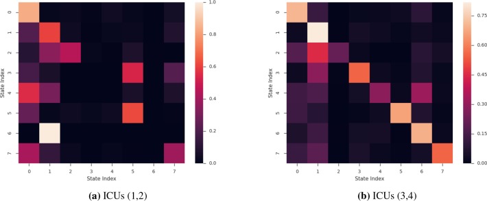
Model Interpretability. We explored the insights that can be drawn from the HMM-based model, namely for the best performing setting. Figure 8 displays the transition matrices, T, that are learned, one for ICUs 1 and 2, and the second for ICUs 3 and 4. From the two heatmaps, we notice that some of the diagonal values are large. This suggests that patients who end up in these states are trapped in them (unlikely to transition to another state). Patients in trapped states are neither getting better or worse and as such remain in the same state for all remaining time points. For example, for patients in ICU 1 or ICU 2 (Figure 8a), if they transition to state 0 at any point in time during their stay, there is very little chance of a transition to any other state. Further analysis comparing the average length of stay of patients who start in state 7 (the most common starting state) and end in state 0 revealed that they had an unusually high LOS compared to the patients who start in state seven and end up in any other state (6.43 days to 4.85 days respectively).

Figure 8:

Heatmap of transition probabilities matrix T for the best-performing HMM

A similar phenomenon holds true for the HMM model trained for ICU 3 and 4. As shown in Figure 8b, the “trapped” state is state one. For the patients who start in state six (the most common starting state), those who end up in state 1 have significantly higher LOS (9.60) compared to those who end up in the other seven states (6.07). This illustrative example shows how the learned parameters can be presented to the physician to make an educated and informed decision.

Discussion and Conclusion

In this paper, we presented an HMM approach to extract latent state features that are later used as regression features to predict the length of stay of patients in ICU. The HMM is learned using irregularly-sampled, multivariate physiological measurements. We introduced several design choices to improve the parameter learning of the HMM models. Our results indicate that the proposed method consistently outperforms most of the existing baseline models. The code for this paper can be found here^g.

While deep learning models can achieve better predictive performance⁴, they require considerably more training samples and can be difficult to interpret. We illustrated the interpretability of the learned latent states as well as the probability transition matrix. Together, they can offer a better understanding of the underlying patient patterns and trends. Moreover, the HMM-based model can succinctly represent the patient’s temporal trend and provide better patient representation.

One potential limitation of our study is the limited number of samples. Although this was mitigated by combining two similar ICUs together, the Physionet 2012 dataset is derived from a larger cohort of patients available in the MIMIC III dataset¹³. Thus a natural step is to confirm our current findings on the entire MIMIC III cohort. We expect that new insights and patterns will be learned through this process, potentially leading to developing a scalable, multi-task HMM-based model for better estimation of the different ICU parameters.

We also note that the learned HMM may still not be dynamic enough, as around 33% of patients start and finish in the same state. This problem also manifests itself in the presence of empty buckets for some start-end state pairs. From the medical perspective, it is unlikely that many of these patients fall into the same group at the beginning given their different health histories and trajectories. We can extend this work to consider a semi-supervision framework to encourage more variability in start-end state pairs, or even auxiliary information (e.g., demographics, socioeconomic status).

Even though the length of stay prediction is an extremely difficult task¹, we showed that an HMM can be used to track multiple physiologic measurements and their interactions over time and elegantly summarize these trends. To accurately learn the new patient representation, we introduced the overlapping time window and ICU type aggregation technique to achieve robust and stable parameter learning of the HMM model. We demonstrated our model’s improved predictive performance on a publicly available dataset of 4000 ICU patients. Future opportunities for improving the estimation progress includes incorporating more samples, developing a multi-task HMM model, and leveraging other patient information.

References

- 1.Nassar AP, Jr, Caruso P. ICU physicians are unable to accurately predict length of stay at admission: a prospective study. International Journal for Quality in Health Care. 2015;28(1):99–103. doi: 10.1093/intqhc/mzv112. [DOI] [PubMed] [Google Scholar]
- 2.Pe´rez A, Chan W, Dennis RJ. Predicting the length of stay of patients admitted for intensive care using a first step analysis. Health Services and Outcomes Research Methodology. 2006;6(3-4):127–138. doi: 10.1007/s10742-006-0009-9. [DOI] [PMC free article] [PubMed] [Google Scholar]
- 3.Maharlou H, Niakan Kalhori SR, Shahbazi S, Ravangard R. Predicting Length of Stay in Intensive Care Units after Cardiac Surgery: Comparison of Artificial Neural Networks and Adaptive Neuro-fuzzy System. Healthcare informatics research. 2018;24(2):109–117. doi: 10.4258/hir.2018.24.2.109. [DOI] [PMC free article] [PubMed] [Google Scholar]
- 4.Harutyunyan H, Khachatrian H, Kale DC, Galstyan A. Multitask learning and benchmarking with clinical time series data. arXiv preprint arXiv:170307771. 2017 doi: 10.1038/s41597-019-0103-9. [DOI] [PMC free article] [PubMed] [Google Scholar]
- 5.Gentimis T, Ala’J A, Durante A, Cook K, Steele R. Predicting Hospital Length of Stay Using Neural Networks on MIMIC III Data. In: Dependable, Autonomic and Secure Computing, 15th Intl Conf on Pervasive Intelligence & Computing, 3rd Intl Conf on Big Data Intelligence and Computing and Cyber Science and Technology Congress (DASC/PiCom/DataCom/CyberSciTech); 2017 IEEE 15th Intl. IEEE; 2017. pp. 1194–1201. [Google Scholar]
- 6.Silva I, Moody G, Scott DJ, Celi LA, Mark RG. Predicting in-hospital mortality of icu patients: The physionet/computing in cardiology challenge 2012. Computing in cardiology. 2012;39:245. [PMC free article] [PubMed] [Google Scholar]
- 7.Macedo E, Malhotra R, Claure-Del Granado R, Fedullo P, Mehta RL. Defining urine output criterion for acute kidney injury in critically ill patients. Nephrology Dialysis Transplantation. 2010;26(2):509–515. doi: 10.1093/ndt/gfq332. [DOI] [PMC free article] [PubMed] [Google Scholar]
- 8.Citi L, Barbieri R. PhysioNet 2012 Challenge: Predicting mortality of ICU patients using a cascaded SVM-GLM paradigm. Computing in Cardiology (CinC); IEEE; 2012. pp. 257–260. [Google Scholar]
- 9.Cooper B, Lipsitch M. The analysis of hospital infection data using hidden Markov models. Biostatistics. 2004 Apr;5(2):223–237. doi: 10.1093/biostatistics/5.2.223. [DOI] [PubMed] [Google Scholar]
- 10.Mannini A, Sabatini AM. Gait phase detection and discrimination between walking–jogging activities using hidden Markov models applied to foot motion data from a gyroscope. Gait & Posture. 2012;36(4):657–661. doi: 10.1016/j.gaitpost.2012.06.017. [DOI] [PubMed] [Google Scholar]
- 11.Sampathkumar H, Chen Xw, Luo B. Mining adverse drug reactions from online healthcare forums using hidden Markov model. BMC Med Inf & Decision Making. 2014;14:91. doi: 10.1186/1472-6947-14-91. [DOI] [PMC free article] [PubMed] [Google Scholar]
- 12.Ridley S, Burchett K, Gunning K, Burns A, Kong A, Wright M, et al. Heterogeneity in intensive care units: fact or fiction? Anaesthesia. 1997;52(6):531–537. doi: 10.1111/j.1365-2222.1997.109-az0109.x. [DOI] [PubMed] [Google Scholar]
- 13.Johnson AE, Pollard TJ, Shen L, Li-wei HL, Feng M, Ghassemi M, et al. MIMIC-III, a freely accessible critical care database. Scientific data. 2016;3:160035. doi: 10.1038/sdata.2016.35. [DOI] [PMC free article] [PubMed] [Google Scholar]