Medial Superior Temporal Area Neurons Respond to Speed Patterns in Optic Flow

Abstract

The speed of visual motion in optic flow fields can provide important cues about self-movement. We have studied the speed sensitivities of 131 neurons in the dorsal region of the medial superior temporal area (MSTd) that responded to either radial or circular optic flow stimuli. The responses of more than two-thirds of these neurons were strongly modulated by changes in the mean speed of motion in optic flow stimuli, with response profiles resembling simple filter characteristics. When we removed the normal gradient of speeds in optic flow (slower speeds in the center, faster speeds in the periphery), approximately two-thirds of the neurons showed changes in their responses. When the speed gradient was altered rather than eliminated, almost nine in 10 neurons preferred either a normal speed gradient or an inverted one (slower speeds near the periphery) over stimuli with no speed gradient. These speed gradient preferences do not come simply from different speed preferences in the central and peripheral segments of the stimulus area. Rather, these speed gradient preferences seemed to reflect interactions between simultaneously presented speeds within an optic flow stimulus. The sensitivity of MSTd neurons to patterns of speed, as well as patterns of direction, strengthens the view that these neurons are well suited to the analysis of optic flow. Sensitivity to speed gradients in optic flow might contribute to neuronal mechanisms for spatial orientation during self-movement and for representing the three-dimensional structure of the visual environment.

Optic flow fields are the global patterns of visual motion generated as an observer moves through the environment (Gibson, 1950). Neurons in the dorsal region of the medial superior temporal area (MSTd) of monkey extrastriate cortex have characteristics suggesting that they might contribute to the analysis of optic flow. Their receptive fields typically cover a quadrant of the visual field, providing access to the global visual motion created by observer movement (Tanaka et al., 1986; Komatsu and Wurtz, 1988). They respond to the planar, radial, and circular patterns, which are the components of optic flow (Saito et al., 1986; Sakata et al., 1986; Tanaka and Saito, 1989; Tanaka et al., 1989; Andersen et al., 1990; Wurtz et al., 1990; Duffy and Wurtz, 1991a,b; Orban et al., 1992; Graziano et al., 1994; Lagae et al., 1994), and many change their responses when the center of motion in optic flow is shifted in the visual field to simulate different headings of observer movement (Duffy and Wurtz, 1995). Finally, some MSTd neurons compensate for the effect of pursuit eye movements that accompany observer movement through the environment (Bradley et al., 1996).

Speed of motion also varies systematically in optic flow stimuli. As an observer moves forward, the pattern of radial expansion typically contains slower motion in the center and faster motion at the edge. Although previous studies have characterized the MSTd neuronal responses to patterns of motion direction, relatively little is known about their responses to patterns of motion speed.Tanaka et al. (1989) showed that withdrawing the speed gradient reduced the response of 34 neurons responding to expanding stimuli by ∼20%.Duffy and Wurtz (1991a) studied 16 neurons and found little effect of speed in all but 3. Orban et al. (1995) found that the speed tuning of 14 neurons could be regarded as being bandpass and that removing the pattern of speeds had little effect. Because speed patterns in optic flow can provide important cues about observer movement (Gibson, 1966;Rogers and Graham, 1979; Cutting et al., 1992), the insensitivity to speed patterns by MSTd neurons would represent an important exception to their suitability for optic flow field analysis.

In light of this relatively limited information on the effects of speed on MSTd neurons, and the importance of speed to optic flow, we studied preferred speeds and the effect of altering speed gradients on a larger sample of MSTd neurons that responded to either expanding or rotating optic flow stimuli. In a sample of 131 neurons, we found that different neurons were tuned to respond to different bands of stimulus speeds, and that the structure of the speed gradient was an important stimulus characteristic in many of these neurons. We believe that this sensitivity of MSTd neurons to patterns of speed, as well as patterns of direction, strengthens the view that these neurons are well suited to contribute to optic flow field analysis.

MATERIALS AND METHODS

Behavioral and neurophysiological techniques. The procedures used in these studies are identical to those reported recently (Duffy and Wurtz, 1995) and are described here only briefly. All protocols were approved by the Institute Animal Care and Use Committee and complied with Public Health Service policy on the humane care and use of laboratory animals.

We recorded the activity of single cortical neurons in two adult rhesus monkeys (Macaca mulatta, 79N and 26K). Scleral search coils were placed in both eyes (Judge et al., 1980), and recording cylinders were placed over trephine holes (anteroposterior, −2; mediolateral, ±15) to access the medial superior temporal area (MST) in both hemispheres. During testing, the monkeys sat in a primate chair while performing a visual fixation task for liquid reward. They fixated a red spot on a 100° × 100° tangent screen 50 cm in front of them, their eye position monitored with the magnetic search coils (Robinson, 1963). Each trial began with the appearance of the red fixation point (light-emitting diode, −0.25° in diameter, 2.7 cd/m²) at the center of the screen, on which the monkey had to fixate within 500 msec and maintain fixation (±2.5°) for up to 3.5 sec. The visual motion stimuli were then projected onto the screen in a pseudorandom sequence, with stimulus durations of 1 sec and interstimulus intervals of 1–1.5 sec.

The activity of single neurons was digitized using a window discriminator and stored with stimulus and behavioral event markers using the REX system (Hays et al., 1982). We recorded neuronal activity using epoxy-coated tungsten microelectrodes that were advanced with a hydraulic microdrive. Neural activity was monitored to locate the depth of physiological landmarks, and studies were initiated whenever neuronal discharges were clearly isolated.

Neuronal response amplitudes were measured as the mean neuronal discharge rate evoked by six repetitions of the 1 sec presentation of each visual motion stimulus. The responses to the visual motion stimuli were compared with activity in the same period of control trials. These control trials were pseudorandomly interleaved with the visual motion trials and consisted of visual fixation without a visual motion stimulus. Differences between stimulated and control trials were tested for statistical significance using Student’s t test (p < 0.01).

At the end of the experiment, electrolytic marking lesions were made along penetration tracks in three guide tubes in each hemisphere. These marks were identified in histological sections 50 μm thick, with every fourth and fifth section stained with Nissl and Gallyas methods. Drawings were made of the sections to locate the electrolytic lesions, relative to anatomic landmarks, to extrapolate the position of the recording sites. These drawings indicate that at least 90% of the neurons studied were in the densely myelinated zone on the anterior bank of the superior temporal sulcus that is included in the MSTd (Komatsu and Wurtz, 1988). The remaining neurons were farther down the anterior bank closer to the lateral region of MST (MSTl), but had the same physiological characteristics.

Visual stimuli. The visual stimuli consisted of 360 white dots on a dark background, randomly distributed at onset, and then moving in the specified pattern. All stimuli covered the 100° × 100° tangent screen with the center of expansion–contraction for radial stimuli, and the center of rotation for circular stimuli, positioned over the fixation point at the center of the screen. Thirteen stimuli were used for preliminary classification of each neuron’s response; these included: eight directions of planar translation (uniform motion in one of eight directions at 45° intervals), two directions of radial motion (inward or outward), two directions of circular motion (clockwise or counterclockwise), and stationary dots. The radial or circular stimulus that evoked the strongest response was identified, without regard to the presence of planar translation responses, and that motion pattern was used in the subsequent speed studies.

In the radial and circular stimuli, dot speed increased with distance from the center of the pattern to create what we term normal speed gradient stimuli. The radial algorithm moved dots inward to, or outward from, the fixation point at the center of the screen, with dot speed increasing as a function of sine(t) × cosine(t), where t is the viewing angle from fixation at the center of the stimulus to a given dot (Fig. 1). This generated a simulation of translational motion away from, or toward, a frontoparallel plane. The circular algorithm moved dots clockwise or counterclockwise around the fixation point at the center of the screen, with dot speed increasing as a tangent function of distance from the center. This generated a simulation of rotational motion with reference to a frontoparallel plane.

Fig. 1.

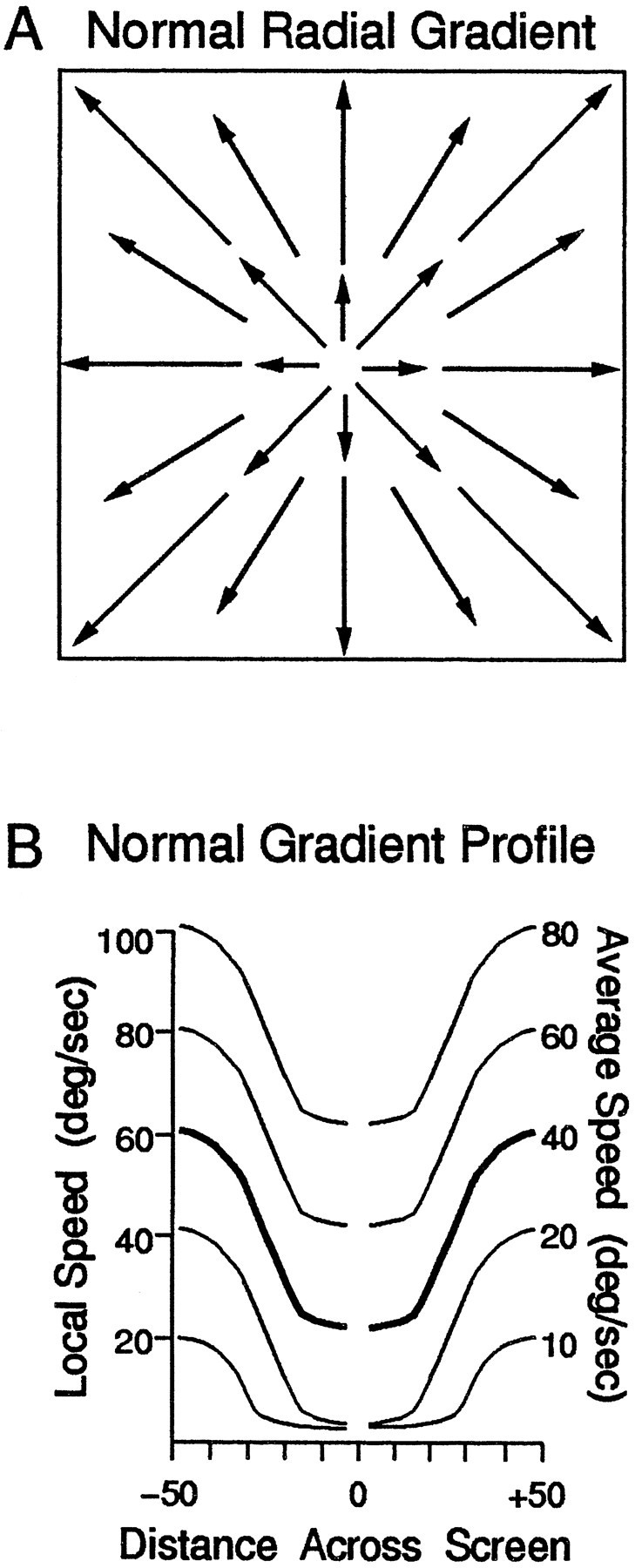
Radial outward motion with a normal speed gradient profile having slower motion near the center and faster motion near the periphery. A, Schematic diagram of the stimuli as projected on the 100° × 100° screen. Arrowsrepresent the direction and speed of dot motion, in this case a radial pattern with faster motion at the edges of the stimulus. Each neuron was tested with the radial (inward or outward) or the circular (counterclockwise or clockwise) stimulus that evoked the strongest response. B, The speed profiles in the five radial stimuli; each profile is shown as a symmetric pair of curves, indicating the pattern of increasing dot speed with distance from the center of the stimulus. The abscissa represents distance from the center of the stimulus, the left ordinate indicates the speed at each location in the stimulus, and the right ordinate indicates the average speed in each stimulus. The gap around the zero position indicates that no dots appeared at the exact center of the screen, because they would be stationary. Speed in radial stimuli is a sine × cosine function of viewing angle from centered fixation to a given dot. Theheavy lines indicate the speed profile in our standard stimulus. Corresponding curves for circular stimuli would be straight lines for dot speed as a linear function of distance from the center of the stimulus.

In the normal gradient stimulus set, the radial and circular stimuli had a mean speed of 40°/sec (Fig. 1B, bold line). This mean speed refers to the speed of the dots at the halfway point between the center and edge of the stimulus. This value was chosen because it yielded subjective comparability of the overall speed in radial, circular, and planar stimuli. Because the dots were evenly distributed, and there is more area beyond the halfway point, the numerical average of dot speeds was above this value. Lower and upper limits were imposed on the dot speeds to minimize apparent stationarity of slow dots (e.g., near the center of outward radial patterns) and the streaking of fast dots (e.g., near the edges of outward radial patterns).

To test for effects of the normal speed gradient, we created nongradient stimuli lacking the dependency of dot speed on distance from the center of the stimulus, maintaining a uniform speed for all dots in a stimulus (Fig. 4A). These uniform speeds matched the mean speeds in the normal gradient speed stimuli. To explore more fully the effects of speed gradients, we applied a scaling factor to the function relating dot speed to distance from the center of the stimulus (Fig. 6). Negative scaling factors (−1.0, −1.5, and −2.0) created inverted gradients in which dot speeds decreased with increasing distance from the center of the stimulus (see Fig.6A). Positive scaling factors created normal (1.0) or exaggerated (1.5 and 2.0) gradients in which dot speeds increased with increasing distance from the center of the stimulus (see Fig.6B). (The nongradient stimuli were implemented using a scaling factor of zero.) This approach was chosen so that all of the local dot speeds were changed while the mean speed (at the halfway point between the center and the edge) remained as a constant, pivotal value.

Fig. 4.

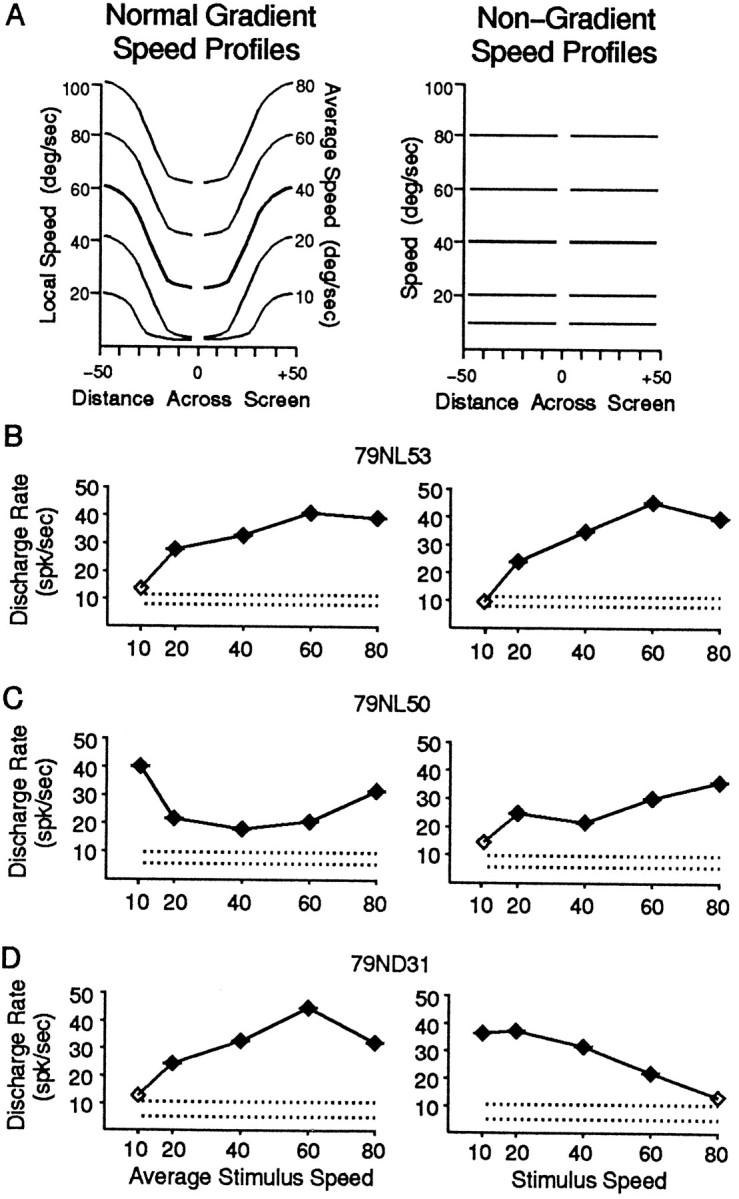
The effects of removing the speed gradient in optic flow stimuli as seen in three neurons that show the range of relationships between responses to normal gradient (left) and nongradient (right) stimuli.A, Stimulus speed profiles showing the relationship between dot speed and location varying as a sine × cosine function in the normal gradient radial stimuli (left) and as a constant speed in nongradient stimuli (right).B, A neuron that showed similar responses across stimulus speeds, regardless of whether the stimuli were the normal gradient speed stimuli (left) or the nongradient speed stimuli (right). C, A neuron that showed different responses at the slowest stimulus speeds, depending on the speed gradient. The 10°/sec stimulus evoked the strongest response with normal gradient stimuli (left) and the weakest response with nongradient stimuli (right).D, A neuron that showed entirely different response profiles depending on the speed gradient. This neuron showed a preference for fast speeds with normal gradient stimuli (left), and a preference for slow speeds with nongradient stimuli (right).

Fig. 6.

Differences in the responses of MSTd neurons to optic flow field stimuli having different speed gradients but the same average speed. A, Graph of the local speeds in the negative gradient speed stimuli, with distance from the center (abscissa) plotted against local speed of dots at that point (left ordinate). The right ordinate indicates the multiplier applied to the normal sine × cosine function that generates these speed gradients. The negative values of these multipliers converted normal gradients, having increasing speed with increasing distance from the center, to negative gradients having decreasing speed with increasing distance from the center. The zero multiplier eliminated the speed gradient to create a nongradient stimulus. B, Graph of the local speeds in the positive gradient speed stimuli, with distance from the center plotted against local speed of dots at that point. Same organization as in A. C, D, Two neurons showing the most common response profiles observed in these studies. The speed gradient multiplier is on the abscissa, and the average response amplitude evoked by that stimulus is on the ordinate.C, The responses of a neuron that showed no significant activation by negative gradient stimuli, and strong activation by positive gradient stimuli. D, The responses of a neuron that showed strong activation by negative gradient stimuli, and weak activation by positive gradient stimuli.

We also made stimuli to explore the basis of speed gradient preferences by testing local speed tuning in different parts of the stimulus area. In creating stimuli that covered only the central 50°² of the screen or the area just beyond it, we imposed a software mask over the appropriate part of the nongradient speed stimuli (Fig. 8). Thus, the total number of dots differed depending on which region was presented, but dot density within the stimulated region was maintained.

Fig. 8.

Comparison of stimulation of center and peripheral areas separately and together for two neurons with strong gradient preferences. Schematic diagrams of the stimuli are shown on theleft, with the responses of two neurons illustrated in the middle and on the right.A, Nongradient speed stimuli containing dot motion at a uniform speed over the central 100° × 100° of the visual field. The nongradient responses are shown with speed (abscissa) plotted against average response amplitude (ordinate). Both neurons showed larger amplitude responses for faster speeds. B, Nongradient speed stimuli were presented in the central 50° × 50° of the stimulus area, and the periphery remained in darkness. The responses of these neurons continue to show larger amplitude responses for faster speeds. C, Nongradient speed stimuli were limited in the stimulus segment outside of the central 50° × 50° of the stimulus area, and the central segment remained in darkness but for the presence of the fixation target. Both neurons continue to show larger amplitude responses for faster speeds. The results inB and C indicate that the response to speed gradients does not appear to reflect different speed preferences in the central and peripheral regions of the field. D, The seven speed gradient stimuli described in Figure 6,A and B, were presented over the central 100° × 100° of the visual field. The neuronal responses are illustrated with the speed gradient multipliers (abscissa) plotted against the average response amplitude evoked by that stimulus (ordinate). The neuron in the middle column shows a preference for negative gradient stimuli, and the one on theright shows a preference for positive gradient stimuli. Very similar speed preferences of these neurons are associated with very different speed gradient preferences.

To test for effects of simultaneously presented speeds, each covering the entire stimulus area, we used the transparent superimposition of a number of normal gradient speed stimuli. This created multiple speed planes with motion parallax effects generated by the motion of each plane relative to that of the other planes (Fig. 12.) The number of dots in each plane was adjusted so that each of the planes had equal numbers of dots, and the total number of dots remained 360.

Fig. 12.

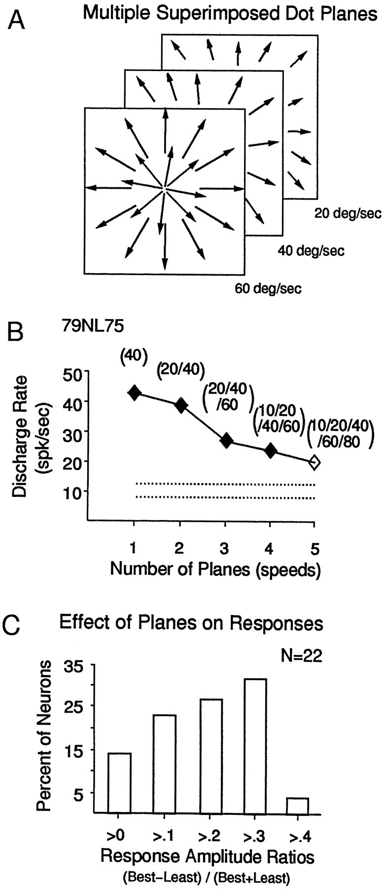
Sensitivity to transparently superimposed optic flow patterns of different average speeds. A, Schematic diagram of three radial patterns with coextensive, transparently superimposed speed gradients, each having increasing speed with increasing distance from the center of the stimulus. B, Responses of an MSTd neuron to multiple speed planes plotted as the number of speed planes (abscissa) versus the mean response amplitude (ordinate). Speeds of each plane are shown inparentheses. Response amplitude decreased with increasing numbers of superimposed speed planes. C, Bar graph showing the percentage of neurons that showed the indicated strength of response preferences for the five multiple-plane stimuli. More than one-third (36%, or 8 of 22) of the neurons showed substantial effects of the number of stimulus planes.

RESULTS

We studied 131 MSTd neurons, first determining the responses of each cell to the visual motion components of optic flow. These component stimuli consisted of 12 patterns covering the central 100° of the visual field: eight planar motion stimuli (eight directions at 45° intervals around 360°), two radial motion stimuli (inward and outward from the fixation point), and two circular motion stimuli (counterclockwise and clockwise around the fixation point). All of these neurons gave significant responses to radial and/or circular motion, with some also responding to planar motion or to radial, circular, and planar motion. Subsequent studies were conducted using the preferred radial or circular stimulus for that neuron.

Effects of mean speed in normal gradient stimuli

We varied the mean speed of radial or circular motion using the same five mean speeds between 10 and 80°/sec for all neurons. In all of these stimuli, we maintained the normal gradient of speed profiles (slower motion in the center) as shown for the example of outward radial motion in Figure 1. More than two-thirds of the neurons that showed some responses to these stimuli (68%, or 83 of 122 neurons) showed strong speed preferences; the amplitude of their response to one speed was at least twice that to another speed. The curves relating response amplitude to mean speed (Fig. 2) showed a variety of shapes that we placed into five categories, which resemble five simple filters. If no response was significantly greater than any other, the neuron was classified as having a flat response profile (broad band; Fig. 2A). If the largest response was at one end of the curve and the smallest response was at the other end, the neuron was classified as having either an increasing or decreasing response profile (low-pass or high-pass; Fig. 2B,C). If the intermediate mean speeds evoked the smallest or largest response, the neuron was classified as having a trough or peak response profile, respectively (bandpass or band-reject; Fig. 2D,E). These response profile classifications do not bear a one-to-one correspondence with classification by optimal stimulus speed (e.g., neurons preferring the fastest speed might show a high-pass or band-reject profile).

Fig. 2.

Five MSTd neurons that illustrate the variety of response profiles to flow fields with different average speeds. These cells all responded best to outward radial motion. The spike density histograms (left) and graphs of mean response amplitude (right) represent averages across six presentations of each stimulus. In the spike density histograms, the abscissa indicates time, with the 1 sec stimulus duration shown as the heavy line below each histogram. The vertical lineindicates neuronal discharge rate, marking stimulus onset, and a response amplitude of 75 spikes/sec. In the graphs, the abscissa indicates the average speed, and the ordinate indicates neuronal discharge rate. The two dashed lines show the average activity level ±1 SD during the unstimulated control trials.Filled symbols mark activity levels that are significantly different from the control activity level (Student’st test; p < 0.01), and theopen symbols mark activity that was not significantly different from control. A, Responses of a neuron that showed no substantial change in activity evoked by stimuli having different average speeds. B, C, Neurons that showed decreasing or increasing response amplitude with increasing average stimulus speed. D, E, Neurons that showed increasing, then decreasing (or the reverse), response amplitude with increasing stimulus speed.

Across the sample, speed had similar effects on the responses to both radial and circular stimuli, and Figure 3A shows the frequency of the five response classes shown in Figure 2. The most common speed response profile is that showing increasing response with increasing mean speed (42% of radial neurons and 38% of circular neurons). The frequency of optimal speed preferences is shown in Figure3B, with the most commonly preferred speeds being the fastest and slowest (64% of radial neurons and 66% of circular neurons). Although we usually tested neurons only to their preferred radial or circular stimuli, those that responded to both had comparable speed profiles to both stimulus patterns. Figure 3C shows the speed profiles of such a neuron that showed preferences for slower stimulus speeds for both radial (left) and circular (right) motion.

Fig. 3.

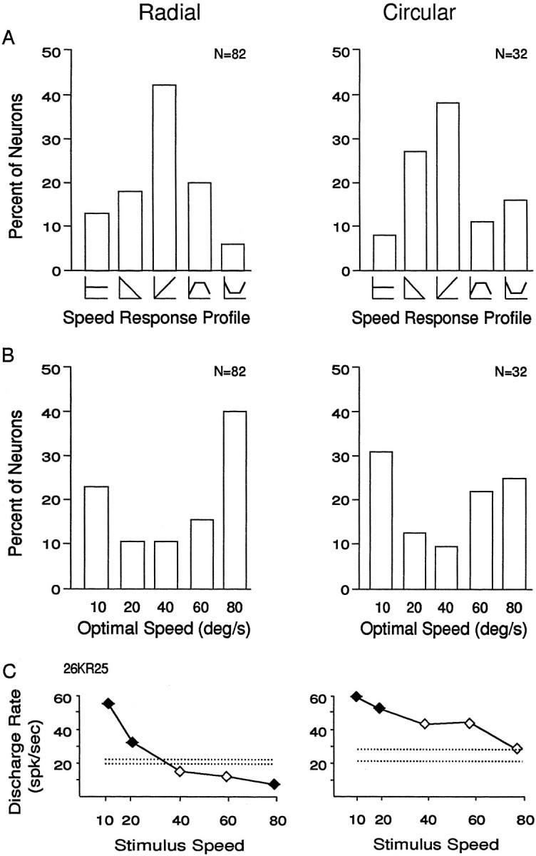
Comparison of speed preferences to radial (left column) and circular (right column) stimuli. A, Percentage of neurons tested with radial and circular stimuli that had each of the five varieties of speed response profiles. A total of 122 neurons showed some response to these stimuli; the 114 neurons that showed at least one statistically significant response were classified into one of five groups. In 13% (11 of 82) of neurons studied with radial stimuli and in 6% (2 of 32) of neurons studied with circular stimuli, no response was statistically significantly greater than any other response; those neurons were considered to have a flat response profile (first bar). In 61% (50 of 82) of neurons studied with radial stimuli and in 66% (21 of 32) of neurons studied with circular stimuli, the strongest response was at one end of the speed range, and the weakest response at the other end, with more neurons in each group preferring faster speeds. The remaining 26% (21 of 82) of neurons studied with radial stimuli and 28% (9 of 32) of neurons studied with circular stimuli either had the smallest response at one end and the peak response at an intermediate speed, or the peak response at one end and the smallest response at an intermediate speed. The classes of response profiles occurred with equal frequency for radial and circular stimuli.B, Percentage of neurons tested with radial and circular stimuli that showed the largest amplitude response at each of the stimulus speeds. The optimal speed (abscissa) was determined by averaging the responses to six stimulus presentations and selecting the speed that evoked the largest average response. A total of 122 neurons were tested with these stimuli, 93% (114 of 122) of which showed statistically significant responses to at least one stimulus. In both the radial and circular groups, the slowest and fastest speeds more commonly evoked the strongest responses, but in both groups there were substantial numbers of neurons preferring each of the speeds.C, Example of a neuron that responded to both radial and circular optic flow stimuli showing the similar preference for slower stimulus speeds for both stimuli. Same format for the graphs as in Figure 2.

Thus, we have made the following observations: (1) the responses of more than two-thirds of the MSTd neurons are strongly modulated by changes in the mean speed of the stimulus gradient; (2) this modulation is equally present for neurons preferring radial or circular stimuli; and (3) the profile of this modulation with change of speeds can be regarded as falling into classes resembling simple filter characteristics.

Effects of speed gradients in optic flow stimuli

In normal gradient stimuli, speed varies as a function of viewing angle from fixation at the center of the stimulus to a given dot: a sine × cosine function for radial stimuli and a tangent function for circular stimuli. To determine whether these speed gradients influence MSTd responses, we created radial and circular stimuli without the normal gradient; i.e., stimuli with the same speed of dot motion throughout the stimulus (Fig. 4A). We see these stimuli with and without the speed gradient as looking alike, but with a clear sense that there are speed differences between them.

We compared the response of 105 neurons to normal gradient and nongradient stimuli at five mean speeds. Overall, the nongradient stimuli evoked only slightly less responsiveness than did the gradient stimuli; approximately two-thirds still showed a response that was at least twice the amplitude of the weakest response (62%, or 58 of 94 for the nongradient stimuli compared with 68% for the gradient stimuli). Figure 4B shows an example of a neuron that responded similarly to the normal gradient (left) and nongradient (right) stimuli. Nevertheless, some neurons showed substantial differences between their responses to normal gradient and nongradient stimuli. For example, the neuron in Figure4C shows a decrease in the response to the lowest speed when the stimulus had no gradient, and the neuron in Figure4D shows a different profile of responses, with a decrease at the fastest speed and an increase at the slowest speed for a nongradient stimulus.

Figure 5 shows the extent of these response differences between normal gradient and nongradient stimuli for our sample of neurons. The preference for faster and (to a lesser extent) slower speeds seen for gradient stimuli is preserved for nongradient stimuli (Fig.5A). When the number of speeds at which the response differs for the normal gradient and the nongradient stimuli are compared (Fig.5B), we find that almost two-thirds of the neurons (64%, or 67 of 105) show significant differences in their responses to at least one of the five speeds. Figure 5C shows the magnitude of the response differences between gradient and nongradient stimuli. Two-thirds of the neurons (69%, or 73 of 105) had speeds at which the larger of the responses to either stimulus was more than one and a half times the amplitude of the smaller response. Thus, in two-thirds of the neurons, the presence of a speed gradient produced substantial changes in neuronal responses.

Fig. 5.

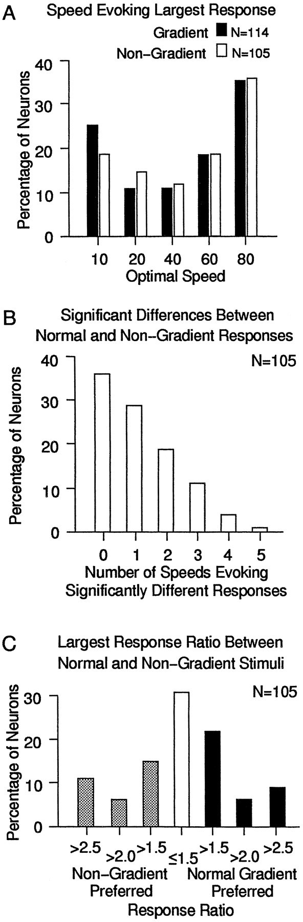
Comparison of responses to normal gradient and nongradient stimuli in the sample of MSTd neurons. A, The percentage of neurons that showed their largest amplitude responses to the indicated speed of nongradient stimuli (open bars) and normal gradient stimuli (solid bars). The graph combines the results for radial and circular motion in Figure3B for the gradient bars and uses the same format as Figure 3B. Removing the gradient had little effect on the overall preference for the fastest and slowest stimulus patterns.B, Percentage of neurons (ordinate) showing statistically significant differences between normal gradient and nongradient responses for the number of speeds indicated on the abscissa. Approximately one-third (36%, or 38 of 105) show no significant differences, almost half (46%, or 48 of 105) show one or two significant differences, and 18% (19 of 105) show three or more differences, usually at one end of the speed range. C, Percentage of neurons showing response magnitude differences expressed as a ratio between normal and nongradient stimuli. The ratio for each cell is at the speed yielding the largest ratio for that neuron. The sample is about evenly divided between those that prefer normal gradients (37%, or 39 of 105; filled bars), those without strong preferences (31%, or 32 of 105; open bar), and those that prefer nongradients (32%, or 34 of 105;shaded bars).

Because eliminating the speed gradient alters the responses of many MSTd neurons, we next determined whether maintaining the gradient but varying its shape also would alter the responses. We used the same mean speed, but for negative speed gradients, the speed decreased with increasing distance from the center of the stimulus (inverted gradients; Fig. 6A), whereas for positive gradients, the speed increased with increasing distance from the center (normal or exaggerated gradients; Fig. 6B). The speed gradients were altered by multiplying the effect of distance from the center by a value from −2 to +2, creating seven speed gradient stimuli covering a segment of the range of naturalistic speed gradients. Figure 6,C and D, shows the responses of two neurons that show the most common response profiles observed. The neuron in Figure6C shows strong responses to the positive speed gradients, in contrast to the neuron in Figure 6D, which shows a clear preference for negative speed gradients.

In 122 MSTd neurons, we found a fairly uniform preference for negative and positive speed gradients (Fig. 7A). All seven gradients are well represented in the sample, with 89% of the neurons preferring either a negative or positive gradient over stimuli with no speed gradient. A somewhat greater number of neurons preferred positive gradients (53%, or 65 of 122) over negative gradients (36%, or 44 of 122), which suggests that the population of neurons might be skewed toward the more commonly encountered self-movement flow fields. To measure the magnitude of the gradient effect, we compared the largest response amplitude to the smallest response amplitude across the seven speed gradients. Figure 7B shows the distribution of the ratios of the largest versus the smallest responses among neurons preferring negative gradients (shaded bars) and neurons preferring positive gradients (filled bars). In both groups, almost half of the neurons (45% for neurons preferring negative gradients, 40% for neurons preferring positive gradients) showed contrast ratios greater than 0.25; i.e., the largest response was more than 1.5 times the amplitude of the smallest response.

Fig. 7.

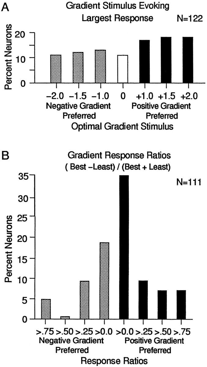
Effect of altering speed gradients on the sample of neurons studied. A, Bar graph showing the percentage of neurons preferring each altered gradient stimulus. More than half of the neurons (53%, or 65 of 122) preferred positive gradients (filled bars), approximately one-third (36%, or 44 of 122) preferred negative gradients (shaded bars), and the remainder (11%, or 13 of 122) preferred the nongradient stimulus. B, Bar graph showing the percentage of neurons with different magnitude responses to the gradient stimuli. The ratio of the largest and smallest responses to the speed gradient stimuli is plotted along the abscissa. Neurons preferring the positive gradients (filled bars) and negative gradients (shaded bars) show a range of contrast ratios, reflecting a continuum from subtle to strong preferences for the stimulus evoking the largest response.

Taken together, these results show that approximately two-thirds of MSTd neurons show substantial effects of eliminating speed gradients and that almost 9 of 10 neurons prefer a positive or inverted speed gradient to stimuli without a speed gradient. This indicates that the spatial distribution of speed across these radial and circular optic flow stimuli can have substantial effects on many MSTd neurons.

Potential explanations of gradient preferences

Speed gradient preferences could result from local differences in speed tuning profiles, such as a preference for slow motion in the center of the stimulus and fast motion in the periphery. To test this hypothesis, we presented stimuli separately to the central 50°² stimulus segment and the peripheral segment outside that area, dividing the stimuli approximately at the point at which local speeds are the same in all of the speed gradients (the pivotal points in Fig. 6A,B). Figure 8 illustrates the results of such experiments in two neurons having distinctly different speed gradient preferences. Both neurons showed increasing responses with increasing speeds in nongradient stimuli covering the full stimulus area (Fig. 8A), and continued to show this same increase whether the stimulus was limited to the central segment of the field (Fig. 8B) or to the peripheral segment (Fig. 8C). Thus, these neurons show no evidence of the kind of substantial differences in central and peripheral speed tuning that would seem necessary to account for the normal speed gradient preferences. This point is reinforced by noting that these neurons had very different speed gradient preferences; neuron 26KL22 showed a strong preference for negative speed gradients (Fig. 8D, left), whereas neuron 26KR5 showed a strong preference for positive speed gradients (Fig. 8D, right).

None of the 48 neurons tested had substantially different speed profiles in the central and peripheral segments. However, we saw substantial differences in overall response amplitude with six neurons showing no significant responses to stimulation of the peripheral segment. The scatter plot in Figure 9 shows the responses of the remaining 42 neurons as the slope from a least squares fit to the response profiles evoked by stimuli in the central (abscissa) and peripheral (ordinate) stimulus segments. Although this measure is insensitive to the details of a few of the response profiles included, it demonstrates the comparability of the responses evoked from the central and peripheral segments (the regression line for the sample has a slope of 0.78; r = 0.77). Thus, we see no evidence of a spatial segregation of speed preferences (e.g., preferring slow motion in the center and faster motion in the periphery) as the basis of speed gradient preferences in MSTd neurons.

Fig. 9.

Comparison of the responses to stimuli restricted to the central or to the peripheral segments of the stimulus for the sample of neurons studied. The scatter plot shows the slopes of the response profiles to stimuli in the central (abscissa) and peripheral (ordinate) stimulus segments. The slopes for central and peripheral movement responses from each neuron were derived from a least squares fit to the response profiles such that they are in units of change in discharge rate/change in stimulus speed. The regression line for the sample has a slope of 0.78 (r= 0.77), reflecting generally similar strengths of speed preferences in the central and peripheral segments.

One factor that might contribute to speed gradient preferences is interactions between responses that are simultaneously evoked from stimuli in different parts of the stimulus area, such as those between the central and peripheral segments. To test this hypothesis, we presented the five speeds of central motion either with no stimuli in the periphery or with slow motion in the periphery. Figure 10 shows the results of such studies in two neurons with nongradient full-field (Fig. 10A), central (Fig. 10B), and peripheral (Fig. 10C) responses, as well as responses to the combination of slow motion (10°/sec) in the periphery with the five speeds tested in the center (Fig. 10D). The middle column shows the responses of a neuron that preferred positive gradient stimuli and that had similar preferences for higher speeds in both central and peripheral stimuli but gave no responses when the periphery contained slow motion, even though the central segment contained the otherwise preferred fast motion. In contrast, the neuron in the right column preferred negative gradient stimuli and had similar preferences for faster speeds in both central and peripheral stimuli, but this neuron’s strongest responses were recorded when the periphery contained slow motion and the central segment contained fast motion. The peripheral stimulus, therefore, clearly can alter the response to different speeds of motion in the central segment.

Fig. 10.

Alteration of responses of two neurons to central segment stimulation by simultaneous stimulation of the peripheral segment. Schematic diagrams of the stimuli are shown on theleft, and the response profiles of two neurons are shown in the middle and on the right with speed (abscissa) plotted against average response amplitude (ordinate).A, Nongradient speed stimuli containing dot motion at a uniform speed over the central 100° × 100° of the visual field. Both neurons show increasing response amplitude with faster stimuli.B, C, Stimuli containing dot motion within the central 50° × 50° of the stimulus, or motion outside the central 50° × 50°. Both neurons show increasing response amplitude with faster speeds in either the central or the peripheral stimulus segment.D, Stimuli containing slow (10°/sec) dot motion outside the central 50° × 50° of the stimulus, and five different speeds within the central 50° × 50° of the stimulus. The neuron in the middle column shows no significant responses to these stimuli, even though central stimulation alone evoked strong responses. The neuron in the right column shows its strongest responses to the combination of fast stimuli in the center and slow motion in the periphery.

To examine such effects more fully, we studied 44 neurons with speed testing in the central segment at our usual five speeds, while either slow motion (as in Fig. 9D) or fast motion was presented in the periphery. The results from the sample are summarized in Figure 11as the slopes of the response profiles for the five speeds in the central segment presented with either slow motion (abscissa) or fast motion (ordinate) in the periphery. The wider distribution of points in Figure 11, with a relatively flat regression line (slope = 0.26) and low correlation coefficient (r = 0.36) (i.e., compared with Fig. 9), reflects substantial differences between the responses to central stimulation when the peripheral segment contained slow versus fast motion. Some neurons appeared activated by fast motion in the periphery, whereas others appeared to be suppressed, and the same is true for slow motion in the periphery. Thus, MSTd neurons have different responses to a local speed stimulus depending on the speed of motion elsewhere in the stimulus, an effect that might contribute to the speed gradient preferences of these neurons.

Fig. 11.

Alteration of the response to stimuli in the central segment by stimuli presented in the peripheral segment. The slopes for slow and fast peripheral movement responses from each neuron were derived from a least squares fit to the response profiles such that they are in units of change in discharge rate/change in central stimulus speed. The scatter plot shows these slopes for the response profiles evoked by central segment stimuli with slow motion in the peripheral segment (abscissa) versus fast motion in the peripheral segment (ordinate). The lack of a clear relationship between the responses to the same central segment stimuli with different speeds in the peripheral segment (sample slope = 0.26; r= 0.37) suggests the presence of interactions between central and peripheral stimuli.

With the stimuli used so far, we have been able to demonstrate speed interactions between spatially segregated parts of the stimulus area. To determine whether such spatial segregation of speeds is needed to elicit speed interactions, we combined different speeds as transparently overlapping planes of optic flow, with each plane having a different mean speed. Such stimuli are shown schematically in Figure12A, with the radial pattern of three nongradient speed planes (20°/sec, 40°/sec, and 60°/sec) shown to indicate transparent overlap throughout the 100°² stimulus area. Figure 12B shows that the responses of a neuron to such overlapping stimuli decrease with increasing numbers of speed planes.

We tested 22 neurons with stimuli containing multiple speed planes and summarized the magnitude of response variation as contrast ratios across multiple-plane stimuli (Fig. 12C). A total of 41% (9 of 22) of the neurons tested showed clear effects of the number of speed planes, with multiple-plane stimuli evoking responses with contrast ratios of more than 0.3 (Fig. 12C, right bar). In the sample, as many neurons preferred decreasing numbers of planes as preferred increasing numbers of planes. Thus, when a number of speeds are presented simultaneously in the same area, MSTd neurons do not respond merely to some preferred speed. Rather, their responses reflect, at least to some degree, the variety of different speeds presented.

The effects of the number of speed planes might rely on the particular speeds in the multiple speed plane stimuli or on the magnitude of the speed difference between those speeds. Figure 13 compares the response to the speed of a single speed plane (A) with the response to the differences between two simultaneously presented speed planes (B) for the same neuron shown in Figure12B. Figure 13A shows the responses to normal gradient stimuli with different mean speeds, whereas Figure13B shows the responses of the same neuron to thedifference between the speeds of two transparently overlapping planes. This neuron gave approximately the same response to all but the slowest single plane stimulus (Fig. 13A), but it showed consistently decreasing responses as speed differences increased between the two-plane stimuli (Fig. 13B). The responses to the difference in the mean speed of two-plane stimuli are not equivalent to the averaged response to those mean speeds in single-plane stimuli. However, the decline in response amplitude with increasing difference between speeds in two-plane stimuli closely resembles the profile for multiple-plane responses in that neuron (Fig.12B). This similarity is consistent with a response of this neuron to the relative motion within the optic flow stimulus.

Fig. 13.

Comparison of the response to the speed of a single speed plane (A) and the speed of the difference between two speed planes (B). A, Responses of the same neuron shown in the previous figure (ordinate) versus mean speed in the normal gradient stimuli (abscissa).B, Responses of the same neuron shown in the previous figure, here as mean response amplitude (ordinates) versus mean speed in the nongradient stimuli (left abscissa) or speed differences in the two-plane stimuli (right abscissa). Speeds of each plane are shown in parentheses. This neuron showed roughly equivalent responses to all but the slowest single-plane stimuli (A), but decreasing responses with greater speed differences in the two-plane stimuli (B), so that the single-plane responses are not clearly similar to responses obtained in two-plane or multiple-plane stimuli. However, there is good agreement between the two-plane responses (right) and the multiple-plane responses (Fig.12B).

We found that neurons that show sensitivity to the relative motion with increasing numbers of planes (Fig. 12B) showed similar profiles of relative motion sensitivity to the speed difference between two superimposed planes of motion (Fig. 13B). Such similarities were evident in seven of the nine neurons that had contrast ratios greater than 0.3 for multiple-plane responses (Fig.12C). Thus, the effects of multiple speed planes can be mimicked by presenting two planes having the same overall differences in speed that are presented in the multiple speed planes stimuli. This does not appear to reflect preferences for a particular speed as much as a preference for a combination of speeds, a preference that might be related to interactions between simultaneously presented speeds.

DISCUSSION

Speed preferences of MSTd neurons

We first examined the sensitivity of MSTd neurons to the pattern of speed in optic flow stimuli by varying the mean speed within the stimuli from 10 to 80°/sec. The radial stimuli would approximate the visual experience of an observer (at our viewing distance of 50 cm from the stimulus) moving forward at speeds from 0.2 to 1.5 m/sec, a range that is included in naturalistic experience. More than two-thirds of the MSTd neurons were strongly modulated by changes in the mean speed of the stimulus, and this modulation was similar in neurons preferring radial stimuli and circular stimuli. The shape of the response profile to stimulus speeds varied across the sample of neurons, but they could be placed into five classes resembling simple filter characteristics. The most common response profile showed increasing response amplitude with increasing mean speed. These findings establish the effect of stimulus speed on the responses of many MSTd neurons, just as previous experiments established the effects of the direction of stimulus motion.

The range of MSTd speed preferences we observed is consistent with those demonstrated by Orban et al. (1995). However, they reported optimal responses mainly in the range of 15–20°/sec, whereas our results (Fig. 3B) suggest that a substantial number of MST neurons prefer faster speeds. It is worth noting that Maunsell and Van Essen (1983) found that neurons in the middle temporal area (MT) also show a broad range of speed preferences, with some neurons preferring slower speeds (10–50°/sec) and others preferring faster speeds (>100°/sec). This conclusion is supported by the broad range of speed preferences demonstrated by Cheng et al. (1994) in MT and V4 neurons.

Our MSTd speed profiles are similar to those reported for striate cortex by Orban et al. (1981), who described speed profiles by analogy to filter characteristics, specifically low-pass, high-pass, and bandpass filters. However, MSTd neurons show an additional profile that can be termed band-reject (Figs. 2E, 3A), in an extension of the analogy to filters. The number of these neurons is small (11% of the total), but their presence might be taken as completing the spectrum of simple filters and might be viewed as supporting a filter model of these responses. The low-pass and high-pass filters provide orthogonal representations of stimulus speed that might interact to create other response characteristics, such as the more selective bandpass and band-reject filters. The band-reject filters are also noteworthy because they might play a role in refining MSTd responses, since a complete set of simple filters provides a greater potential for focusing bandwidth to complex stimuli. The range of MSTd response profiles is also consistent with the observation that response profile shape varies along a continuum in MT (Maunsell and Van Essen, 1983).

The most salient point is that many MSTd neurons are sensitive to the mean speed of the optic flow stimulus, which is in contrast to the impression given by several previous studies of MSTd, including our own (Duffy and Wurtz, 1991a), based on much smaller samples of neurons.

Effects of speed gradients

To assess the effects of speed gradients, we created stimuli with the same radial and circular patterns of motion direction, but with no speed gradient (Fig. 4), inverted speed gradients (faster motion in the center than in the periphery; Fig. 6A), or exaggerated gradients (much slower motion in the center; Fig.6B). Approximately two-thirds of the MSTd neurons showed substantial effects of eliminating speed gradients, and almost 9 of 10 neurons preferred a positive gradient or inverted speed gradient to stimuli having no speed gradient. This indicates that the spatial distribution of speed across optic flow stimuli has substantial effects on many MSTd neurons and could contribute to the role these neurons play in the analysis of optic flow.

This conclusion differs from those of previous studies in ways that may be accounted for by differences in the experiments and in the size of the sample of neurons. In the first study of speed gradient effects on MSTd neurons (Tanaka et al., 1989), one of eight radial segments in an expansion/contraction stimulus was modified to eliminate the local speed gradient, and little effect was observed. We were able to present a series of gradient stimuli that cover more of the natural range of speed gradients in optic flow, and this may have revealed effects that otherwise would not be apparent. In addition, our sample contained some MSTd neurons with relatively little sensitivity to speed, raising the possibility that studies with smaller sample sizes might have included such neurons.

We altered speed in optic flow stimuli to determine whether MSTd neurons might use this parameter as a cue for self-movement perception. However, these stimuli might also be interpreted as simulating the movement of large objects at various speeds relative to a stationary observer. Our findings revealed a third potential role for MSTd neurons: the analysis of visual motion cues about the three-dimensional structure of the environment. For example, MSTd neurons preferring positive speed gradients might be most active when nearby features of the scene are in the peripheral visual field (i.e., the trees lining the approach to the house in Fig. 14A) with remote features in the central visual field (i.e., the house in Fig.14A). In contrast, neurons preferring negative speed gradients might be most active when nearby features are in the central visual field (i.e., the house in Fig. 14B) with remote features in the periphery (i.e., the trees in Fig.14B). This interpretation suggests that MSTd neurons might contribute to previously demonstrated perceptual capacities to discriminate between differently structured environments based on the visual motion in optic flow (Braunstein and Andersen, 1981; Harris et al., 1992). These findings are also consistent with the notion that MSTd neurons could serve as the hypothesized higher-order elements needed to integrate speed and direction information from optic flow to support visual space perception (Nakayama and Loomis, 1974).

Fig. 14.

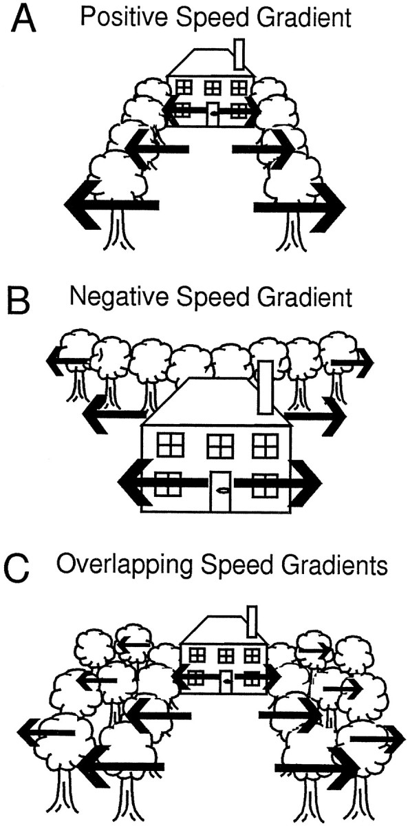
Schematic illustrations of naturalistic circumstances in which an observer moving toward the center of the scene would encounter positive (A), negative (B), and overlapping (C) speed gradients.A, When nearby features of the scene are in the peripheral visual field (the trees lining the approach to the house), and increasingly remote features are closer to the center of the visual field (the house), the observer would encounter a positive speed gradient. As indicated by the length of the arrows, the speed of feature motion would increase from the center to the periphery. B, When nearby features of the scene are in the central visual field (the house) and remote features are in the periphery visual field (the trees), the observer would encounter a negative speed gradient. As indicated by the length of thearrows, the speed of feature motion would decrease from the center to the periphery. C, When remote features are in the central visual field (the house), and the peripheral visual field contains features at substantially varying distances (the trees), the observer sees overlapping positive speed gradients. As indicated by the length of the arrows, there would be a general increase in speed of feature motion from the center to the periphery. In addition, the overlapping gradients would create motion parallax in the scene, as indicated by the decreasing length ofarrows over trees positioned at increasing distances from the observer.

Speed interactions in MSTd neurons

A simple explanation of speed gradient preferences would be that central and peripheral stimulus segments have different speed preferences (e.g., preferring slow movement in the center and fast movement in the periphery). We compared responses evoked by stimuli in the central 50°² of the stimulus area with those evoked by stimuli outside that area and found no substantial differences in their speed profiles (Fig. 9). Furthermore, neurons with very different gradient preferences were found to have very similar central and peripheral speed profiles (Fig. 8A–D).

The absence of support for the simplest explanation of speed gradient preferences prompted us to consider whether interactions between speeds simultaneously presented in the central and peripheral stimulus segments might shape the responses of these neurons. To test this hypothesis, we compared the speed profiles evoked by stimuli in the central segment when presented along with either slow or fast motion in the periphery. In most of the neurons tested with these stimuli, there were substantial differences between responses to stimuli presented in the central segment, depending on the speed of motion in the periphery (Figs. 10, 11). Such interactions could contribute to speed gradient preferences by altering responses to particular combinations of central and peripheral speeds.

Because these experiments suggested that speed gradient preferences might rely on interactions between simultaneously presented speed stimuli, we wanted to determine whether those interactions required some particular spatial structure of the stimuli (e.g., slow motion in the center and fast motion in the periphery). To test this possibility, we presented different speeds together as transparently overlapping speed planes each covering the entire stimulus area (Fig.12A). We found that 41% of the neurons showed substantial changes in response amplitude as the number of speed planes increased from one to five (Fig. 12B,C), with similar effects induced by increasing the magnitude of the speed difference between two overlapping speed planes (Fig. 13). Thus, there is evidence for speed interactions even in the absence of the spatial separation of speeds in the stimulus.

The perceptual utility of neuronal sensitivity to the overlap of multiple speed planes might relate to the motion parallax in these stimuli. Figure 14C illustrates how a visual scene with substantial depth of field (i.e., the trees at various distances from the approach to the house) presents spatially overlapping features at different speeds. Motion parallax can reflect the three-dimensional structure of the environment (Gibson, 1966) and support detection of heading direction during self-movement (Rogers and Graham, 1979;Cutting et al., 1992), possibly relating the speed and direction preferences of MSTd neurons. Our experiments provide some clues about motion interactions that might underlie speed gradient and speed overlap preferences in MST neurons. However, further studies in which these preferences and interaction effects are tested together in a substantial number of neurons would be required to characterize the underlying mechanisms.

REFERENCES

- 1.Andersen RA, Snowden RJ, Treue S, Graziano M. Hierarchical processing of motion in the visual cortex of monkey. Cold Spring Harb Symp Quant Biol. 1990;55:741–748. doi: 10.1101/sqb.1990.055.01.069. [DOI] [PubMed] [Google Scholar]
- 2.Bradley DC, Maxwell M, Andersen RA, Banks MS, Shenoy KV. Mechanisms of heading perception in primate visual cortex. Science. 1996;273:1544–1547. doi: 10.1126/science.273.5281.1544. [DOI] [PubMed] [Google Scholar]
- 3.Braunstein ML, Andersen GJ. Velocity gradients and relative depth perception. Percept Psychophys. 1981;29:145–155. doi: 10.3758/bf03207278. [DOI] [PubMed] [Google Scholar]
- 4.Cheng K, Hasegawa T, Saleem KS, Tanaka K. Comparison of neuronal selectivity for stimulus speed, length, and contrast in the prestriate visual cortical areas V4 and MT of the macaque monkey. J Neurophysiol. 1994;71:2269–2280. doi: 10.1152/jn.1994.71.6.2269. [DOI] [PubMed] [Google Scholar]
- 5.Cutting JE, Springer K, Braren PA, Johnson SH. Wayfinding on foot from information in retinal, not optical, flow. J Exp Psychol Gen. 1992;121:41–72. doi: 10.1037//0096-3445.121.1.41. [DOI] [PubMed] [Google Scholar]
- 6.Duffy CJ, Wurtz RH. Sensitivity of MST neurons to optic flow stimuli. I. A continuum of response selectivity to large-field stimuli. J Neurophys. 1991a;65:1329–1345. doi: 10.1152/jn.1991.65.6.1329. [DOI] [PubMed] [Google Scholar]
- 7.Duffy CJ, Wurtz RH. Sensitivity of MST neurons to optic flow stimuli. II. Mechanisms of response selectivity revealed by small-field stimuli. J Neurophys. 1991b;65:1346–1359. doi: 10.1152/jn.1991.65.6.1346. [DOI] [PubMed] [Google Scholar]
- 8.Duffy CJ, Wurtz RH. Response of monkey MST neurons to optic flow stimuli with shifted centers of motion. J Neurosci. 1995;15:5192–5208. doi: 10.1523/JNEUROSCI.15-07-05192.1995. [DOI] [PMC free article] [PubMed] [Google Scholar]
- 9.Gibson JJ. The perception of the visual world. Houghton Mifflin; Boston: 1950. [Google Scholar]
- 10.Gibson JJ. The senses considered as perceptual systems. Houghton Mifflin; Boston: 1966. [Google Scholar]
- 11.Graziano MSA, Andersen RA, Snowden RJ. Tuning of MST neurons to spiral motion. J Neurosci. 1994;14:54–67. doi: 10.1523/JNEUROSCI.14-01-00054.1994. [DOI] [PMC free article] [PubMed] [Google Scholar]
- 12.Harris M, Freeman T, Hughes J. Retinal speed gradients and the perception of surface slant. Vision Res. 1992;32:587–590. doi: 10.1016/0042-6989(92)90252-e. [DOI] [PubMed] [Google Scholar]
- 13.Hays AV, Richmond BJ, Optican LM. A UNIX- based multiple process system for real-time data acquisition and control. WESCON Conference Proceedings. 1982;2:1–10. [Google Scholar]
- 14.Judge SJ, Richmond BJ, Chu FC. Implantation of magnetic search coils for measurement of eye position: an improved method. Vision Res. 1980;20:535–538. doi: 10.1016/0042-6989(80)90128-5. [DOI] [PubMed] [Google Scholar]
- 15.Komatsu H, Wurtz RH. Relation of cortical areas MT and MST to pursuit eye movements. I. Localization and visual properties of neurons. J Neurophysiol. 1988;60:580–603. doi: 10.1152/jn.1988.60.2.580. [DOI] [PubMed] [Google Scholar]
- 16.Lagae L, Maes H, Raiguel S, Xiao D-K, Orban GA. Responses of macaque STS neurons to optic flow components: a comparison of areas MT and MST. J Neurophysiol. 1994;71:1597–1626. doi: 10.1152/jn.1994.71.5.1597. [DOI] [PubMed] [Google Scholar]
- 17.Maunsell JHR, Van Essen DC. Functional properties of neurons in middle temporal visual area of the macaque monkey. I. Selectivity for stimulus direction, speed, and orientation. J Neurophysiol. 1983;49:1127–1147. doi: 10.1152/jn.1983.49.5.1127. [DOI] [PubMed] [Google Scholar]
- 18.Nakayama K, Loomis JM. Optical velocity patterns, velocity-sensitive neurons, and space perception: a hypothesis. Perception. 1974;3:63–80. doi: 10.1068/p030063. [DOI] [PubMed] [Google Scholar]
- 19.Orban GA, Kennedy H, Maes H. Response to movement of neurons in areas 17 and 18 of the cat: velocity sensitivity. J Neurophysiol. 1981;45:1043–1058. doi: 10.1152/jn.1981.45.6.1043. [DOI] [PubMed] [Google Scholar]
- 20.Orban GA, Lagae L, Verri A, Raiguel S, Xiao D, Maes H, Torre V. First-order analysis of optical flow in monkey brain. Proc Natl Acad Sci USA. 1992;89:2595–2599. doi: 10.1073/pnas.89.7.2595. [DOI] [PMC free article] [PubMed] [Google Scholar]
- 21.Orban GA, Lagae L, Raiguel S, Xiao D, Maes H. The speed tuning of medial superior temporal (MST) cell responses to optic-flow components. Perception. 1995;24:269–285. doi: 10.1068/p240269. [DOI] [PubMed] [Google Scholar]
- 22.Robinson DA. A method of measuring eye movement using a scleral search coil in a magnetic field. IEEE Trans Biomed Eng. 1963;10:137–145. doi: 10.1109/tbmel.1963.4322822. [DOI] [PubMed] [Google Scholar]
- 23.Rogers B, Graham M. Motion parallax as an independent cue for depth perception. Perception. 1979;8:125–134. doi: 10.1068/p080125. [DOI] [PubMed] [Google Scholar]
- 24.Saito H-A, Yukie M, Tanaka K, Hikosaka K, Fukada Y, Iwai E. Integration of direction signals of image motion in the superior temporal sulcus of the macaque monkey. J Neurosci. 1986;6:145–157. doi: 10.1523/JNEUROSCI.06-01-00145.1986. [DOI] [PMC free article] [PubMed] [Google Scholar]
- 25.Sakata H, Shibutani H, Ito Y, Tsurugai K. Parietal cortical neurons responding to rotatory movement of visual stimulus in space. Exp Brain Res. 1986;61:658–663. doi: 10.1007/BF00237594. [DOI] [PubMed] [Google Scholar]
- 26.Tanaka K, Saito H. Analysis of motion of the visual field by direction, expansion/contraction, and rotation cells clustered in the dorsal part of the medial superior temporal area of the macaque monkey. J Neurophysiol. 1989;62:626–641. doi: 10.1152/jn.1989.62.3.626. [DOI] [PubMed] [Google Scholar]
- 27.Tanaka K, Hikosaka K, Saito H-A, Yukie M, Fukada Y, Iwai E. Analysis of local and wide-field movements in the superior temporal visual areas of the macaque monkey. J Neurosci. 1986;6:134–144. doi: 10.1523/JNEUROSCI.06-01-00134.1986. [DOI] [PMC free article] [PubMed] [Google Scholar]
- 28.Tanaka K, Fukuda Y, Saito H. Underlying mechanisms of the response specificity of expansion/contraction and rotation cells in the dorsal part of the medial superior temporal area of the macaque monkey. J Neurophysiol. 1989;62:642–656. doi: 10.1152/jn.1989.62.3.642. [DOI] [PubMed] [Google Scholar]
- 29.Wurtz RH, Yamasaki DS, Duffy CJ, Roy J-P. Functional specialization for visual motion processing in primate cerebral cortex. Cold Spring Harb Symp Quant Biol. 1990;55:717–727. doi: 10.1101/sqb.1990.055.01.067. [DOI] [PubMed] [Google Scholar]