Spatial Relationships among Three Columnar Systems in Cat Area 17

Abstract

In the primary visual cortex, neurons with similar response properties are arranged in columns. As more and more columnar systems are discovered it becomes increasingly important to establish the rules that govern the geometric relationships between different columns. As a first step to examine this issue we investigated the spatial relationships between the orientation, ocular dominance, and spatial frequency domains in cat area 17. Using optical imaging of intrinsic signals we obtained high resolution maps for each of these stimulus features from the same cortical regions. We found clear relationships between orientation and ocular dominance columns: many iso-orientation lines intersected the borders between ocular dominance borders at right angles, and orientation singularities were concentrated in the center regions of the ocular dominance columns. Similar, albeit weaker geometric relationships were observed between the orientation and spatial frequency domains. The ocular dominance and spatial frequency maps were also found to be spatially related: there was a tendency for the low spatial frequency domains to avoid the border regions of the ocular dominance columns. This specific arrangement of the different columnar systems might ensure that all possible combinations of stimulus features are represented at least once in any given region of the visual cortex, thus avoiding the occurrence of functional blind spots for a particular stimulus attribute in the visual field.

A characteristic feature of the cortex is that neurons with similar response properties are clustered together in columns extending radially through the whole thickness of the cortex. In the visual cortex it has been recognized early on that neurons are grouped according to their key response properties, orientation preference, and ocular dominance (Hubel and Wiesel, 1962,1963). The observation of multiple columnar systems in the primary visual cortex gave rise to the question of how these different columns are arranged within the cortex. Mainly on the basis of electrophysiological and anatomical observations, Hubel and Wiesel (1977) proposed a model for the functional architecture of monkey primary visual cortex, the so called “ice-cube” model. Key to this model is the concept of a modular organization: the visual cortex was proposed to be composed of a large number of more or less identical elementary processing units, with each of these modules containing the complete machinery for the analysis of a small part of the visual field with respect to all possible stimulus features. Later, with the detection of the cytochrome oxidase blobs as a specialized system devoted to the processing of color information in primates, the ice-cube model was extended to include blobs within each module (Livingstone and Hubel, 1984).

In recent years increasing evidence has accumulated that in addition to orientation, ocular dominance, and color selectivity neurons in the visual cortex are organized in columns with respect to other stimulus parameters, such as direction of movement (Payne et al., 1981; Tolhurst et al., 1981; Swindale et al., 1987; Shmuel and Grinvald, 1996; Weliky et al., 1996), spatial frequency (Tootell et al., 1981, 1988; Shoham et al., 1997), disparity (LeVay and Voigt, 1988), and stimulus on- or offset [so far shown only for LGN-afferents (McConnell and LeVay, 1984; Zahs and Stryker, 1988; Gordon et al., 1993)]. The concept of a modular architecture in a strict sense is challenged by the discovery of this multitude of columns in the visual cortex, because it is difficult to imagine how every elementary processing unit could house the different types of columns in a way that all possible combinations of stimulus features are represented at least once in each module. If a combination of stimulus representations were missing in a module, a blind spot for this specific stimulus at this particular location in the visual field would result. It is therefore important to determine how the various columnar systems are spatially related to each other.

In the visual cortex of macaques, geometric relationships between ocular dominance and orientation columns have been demonstrated (Bartfeld and Grinvald, 1992; Obermayer and Blasdel, 1993; Blasdel et al., 1995). In cat visual cortex the layout of ocular dominance columns is much more irregular than in the macaque. We were thus wondering whether geometric relationships between ocular dominance and orientation columns would also exist in the cat. When we first imaged ocular dominance and orientation columns in the cat we suggested that the centers of pinwheels may lie in the middle of ocular dominance columns just like in the macaque, but we pointed out that additional experiments were required (Bonhoeffer et al., 1995; Hübener et al., 1995). Here we report the results of such experiments establishing our suggestion, which has been independently confirmed recently (Crair et al., 1997). Moreover, the visual cortex of the cat contains another functional map that seemed interesting to us in this respect. A spatial frequency map has been demonstrated by Tootell et al. (1981) using the 2-deoxyglucose technique, and we have recently shown, using optical imaging, that the spatial frequency map is actually a spatiotemporal frequency map composed of two sets of distinct functional domains (Shoham et al., 1997).

Here we use optical imaging of intrinsic signals (Grinvald et al., 1986; Frostig et al., 1990; Ts’o et al., 1990) to analyze the geometric relationships between orientation, ocular dominance, and spatial frequency domains in cat area 17.

Preliminary results have been published previously in abstract form (Hübener et al., 1995; Shoham et al., 1995).

MATERIALS AND METHODS

Optical imaging of intrinsic signals was used to visualize functional maps in the primary visual cortex (area 17) of 13 cats ranging in age from 2 to 5 months. Most experiments were performed on 2- or 3-month-old cats. The rationale for using young animals was that the signal-to-noise ratio of the optical signals was often larger than in adult animals. This was particularly true when ocular dominance and spatial frequency maps were imaged. A comprehensive description of the techniques used in this study can be found in Bonhoeffer and Grinvald (1996).

Optical imaging. Animals were initially anesthetized with ketamine (15–30 mg/kg, i.m.) and xylazine (1.5–2 mg/kg, i.m.) supplemented by atropine (0.15 mg/kg, i.m.). A tracheotomy was performed, and the cats were artificially respirated (40–50% N₂O, 50–60% O₂, 0.8–1.5% halothane). Electrocardiogram, electroencephalogram, arterial oxygen saturation (SpO₂), and rectal temperature were monitored throughout the experiment. The end-tidal CO₂ was measured and kept at ∼3.5% by adjusting the rate and volume of the respirator. Relaxation was accomplished by intravenous infusion of gallamine triethiodide (30 mg · kg⁻¹ · hr⁻¹). The pupils were dilated with atropine (0.5%), and the nictitating membranes were retracted with neosynephrine (2%). The eyes were refracted carefully with a refractometer and corrected with appropriate contact lenses to focus them onto a tangent screen 1 m in front of the animal. A trepanation between Horsley–Clarke coordinates P4 and P10 was performed above area 17 of each hemisphere. A stainless steel chamber was cemented onto the skull, and the inner margin of the chamber was sealed with wax. After careful removal of the dura the chamber was filled with silicone oil and sealed with a coverglass.

The cortex was illuminated with red light (peak transmission: 707 nm) by means of two flexible light guides. A Peltier cooled, slow-scan CCD camera (Princeton Instruments, Trenton, NJ, or Theta System–ORA 2001, Optical Imaging, Germantown, NY) equipped with a tandem lens arrangement (Ratzlaff and Grinvald, 1991) was adjusted with its image plane parallel to and 500 μm below the cortical surface. Images were acquired while the animal was visually stimulated, with each individual stimulus presentation lasting 3 sec. During this period five frames, each 600 msec long, were captured, digitized (12 bit), and written to the computer’s hard drive.

Visual stimulation. Large field stimuli (80° wide, 60° high) were generated with the program “Stim” (Kaare Christian, The Rockefeller University) and projected onto a frosted glass screen with a video projector. Stimuli consisted of high-contrast (90%) square-wave gratings presented at four orientations and two spatial frequencies (usually 0.2 cycles/degree and 0.6 cycles/degree) in a pseudo-random sequence. During each presentation the grating was moved back and forth at different speeds (10°/sec and 3.3°/sec) that were chosen to keep the temporal frequency constant for all stimuli (at 2 Hz). Computer-controlled shutters in front of the eyes allowed for randomly alternating monocular stimulation. Each individual stimulus cycle consisted of 3 sec of moving stimulus, during which data were acquired, followed by a period of 7 sec to allow the signal to return to baseline. During this 7 sec period the grating that was to be drifted during the next stimulus cycle was placed on the screen and held stationary. This standing–moving sequence was chosen to avoid unwanted stimulus-on responses during the data acquisition period. Depending on the noise level of the functional maps, each stimulus was repeated between 32 and 160 times. The responses to 16 identical stimuli were accumulated on line, with the resulting reflectance image serving as the basic data set for the computation of functional maps.

Computation of functional maps. In most cases we discarded the first frame captured during each stimulus presentation, because it usually contained almost no stimulus-related signal. As the next step in data analysis, “single-condition maps” were calculated in the “cocktail blank” mode (Bonhoeffer and Grinvald, 1993). To this end the reflectance image obtained with one stimulus (in fact 16 repetitions of one stimulus; see above) was divided by the sum of the images obtained with all stimuli. Then, after verifying that all single-condition maps for a particular stimulus were reproducible, they were averaged to improve the signal-to-noise ratio. Iso-orientation maps were computed analogous to the single-condition maps; that is, the sum of the images acquired with one orientation was divided by the sum of the images acquired with all orientations. The iso-orientation maps were then used to generate a map visualizing the layout of orientation preference across the visual cortex. These color-coded orientation preference maps were calculated by vectorially summing, for each pixel, the responses to all orientations and displaying the angle of the resulting vector in color (Blasdel and Salama, 1986). Differential ocular dominance maps were calculated by adding all single-condition maps obtained with stimulation of the contralateral eye and dividing the result by the sum of the maps of the ipsilateral eye. Similarly, spatial frequency maps were computed by dividing the sum of the single-condition maps of one spatial frequency by the sum of the maps of the second spatial frequency.

Quantitative analysis of geometric relationships. The geometric relationships between the different columnar systems were assessed with a detailed quantitative analysis. The intersection angles of iso-orientation lines with ocular dominance borders were determined by computing, for both maps, the gradient fields. The angular difference between the two gradient fields corresponded to the intersection angles at the different locations of the map. This calculation was applied only to pixels located on borders between ocular dominance columns. In a similar way we computed the intersection angles between iso-orientation lines and borders between spatial frequency domains.

To determine the positions of the pinwheel-centers with respect to the ocular dominance and spatial frequency domains, we first had to locate the pinwheel-centers. To this end, for each point in the vectorial orientation preference map we calculated the sum of the absolute values of divergence and curl. Next we searched for local maxima in the resulting array and sorted these maxima in descending order of value. Then we applied a threshold to discard, under visual control, all maxima below a certain value that were not located on pinwheel-centers. With this standardized procedure we were able to find the exact positions of all pinwheel-centers in the orientation preference maps. The center and border regions of ocular dominance columns were defined by way of the pixel values in the differential maps. Each map was divided into 10 regions of equal area, with those parts encompassing the pixels with the lowest or highest values corresponding to the centers of the contralateral or ipsilateral eye columns. Thus, the combined center regions made up 20% of the area of an ocular dominance map. Accordingly, the border regions were defined as 20% of the area of a map with intermediate pixel values. The center and border regions of the spatial frequency domains were defined in the same manner. It should be noted that this definition of the “centers” of domains is a functional rather than a geometrical one.

To analyze the relationships between low spatial frequency domains [and thus the cytochrome oxidase blobs (Shoham et al., 1997)] and ocular dominance columns we first located the centers of the low spatial frequency domains. To this end we used an algorithm searching for local minima in the low-pass-filtered spatial frequency map. The relative frequencies of these centers in different regions of the ocular dominance maps were then determined.

All statistical testing was done under the assumption of two-tailed distributions; the average values are given as mean ± SEM.

RESULTS

Ocular dominance columns

To visualize ocular dominance columns with optical imaging, we presented grating stimuli of four different orientations to each eye separately in a randomly interleaved manner. All orientations were presented at two spatial frequencies. Figure1A–H shows the resulting eight iso-orientation maps from one such experiment. In each map the dark patches are those regions of the cortex that were activated by the respective stimulus. Iso-orientation domains obtained with monocular stimulation appear as round or elongated and sometimes irregularly shaped patches with a width of ∼0.5 mm and a center-to-center spacing of ∼1 mm. A comparison of the contra- and ipsilateral orientation maps at a given orientation reveals that the two corresponding maps have a different layout, reflecting the well known segregation into ocular dominance columns. A more detailed inspection of these pairs of maps reveals that most of the orientation domains in one of the maps are located in close proximity to domains in the map of the other eye. To facilitate comparison of the contra- and ipsilateral orientation maps at one orientation we have outlined the patches in the 135° map of the contralateral eye (Fig.1D) and overlaid these outlines on the ipsilateral orientation map (Fig. 1H). As can be seen, the maps are clearly different, but in some instances patches in the contralateral orientation map are partially overlapping with patches in the ipsilateral orientation map. Such regions of overlap are thus more or less equally well activated by stimulation via the left or the right eye.

Fig. 1.

Monocular stimulation of the contra- and ipsilateral eye produces different activity patterns in cat area 17.A–H, Iso-orientation maps obtained after monocular stimulation with gratings of four different orientations. Thedark patches denote regions that were activated by the respective stimulus. Active regions in the contralateral 135° map shown in D were outlined and transferred to the corresponding ipsilateral map in H to facilitate comparison. Both maps are clearly different, thus suggesting also a segregation according to ocular dominance. I, Cortical blood vessel pattern of the imaged region. A, Anterior;P, posterior; M, medial;L, lateral. Scale bar, 1 mm.

From the eight maps shown in Figure 1 we then calculated two functional maps: the orientation-preference “angle map” (Fig.2A) and the ocular dominance map (Fig. 2B). For the orientation-preference map we first added the contra- and ipsilateral orientation maps for each of the four orientations and then used vector addition to produce the angle map in which the preferred orientation is color-coded according to the oriented bars shown in Figure2A (right). The patchy character of the orientation columns becomes obvious again. As described previously (Bonhoeffer and Grinvald, 1991, 1993; Bonhoeffer et al., 1995), the leading theme of the spatial organization of the orientation domains in cat visual cortex is that they are arranged in a pinwheel-like manner around singularity points. Many of these pinwheels, approximately half with clockwise and half with counterclockwise succession of orientation domains, can be identified in the map shown in Figure2A.

Fig. 2.

Orientation preference “angle map” and ocular dominance map from the same patch of cortex. A, Orientation preference map calculated from the iso-orientation maps shown in Figure 1. The angle of the preferred orientation is color-coded according to the key shown on the right. As described previously, orientation domains are organized in a pinwheel-like manner. B, Ocular dominance map. Blackcodes for contralateral and white for ipsilateral eye preference. The layout of the ocular dominance map is clearly different from that of the iso-orientation maps shown in Figure 1. Scale bar, 1 mm.

The ocular dominance map (Fig. 2B) was calculated by adding up all four iso-orientation maps of the contralateral eye and dividing the result by the sum of the four maps of the ipsilateral eye. Thus, in this map black codes for contralateral eye preference, and white codes for ipsilateral eye preference. One can see immediately that the layout of the ocular dominance map differs strongly from that of the iso-orientation maps shown in Figure 1. The ocular dominance columns have the shape of curved bands running across the cortex over a distance of a few millimeters. The width of individual bands in this map is fairly constant, in most instances between 0.4 and 0.5 mm. We observed, however, a considerable amount of variability between maps from different cats, as can be seen in Figure3, which shows ocular dominance maps from two other animals. In these maps the spacing of the ocular dominance columns is wider on average; in some cases the bands have a width of up to 1 mm. Compared with the ocular dominance map presented in Figure 2the general layout of the maps shown in Figure 3 seems to be more irregular, with strong fluctuations in the width of individual bands giving them a beaded appearance.

Fig. 3.

Variability in the width and shape of ocular dominance bands between animals. A, B, Ocular dominance maps from two additional cats. Black regions were activated stronger by the contralateral eye. Compared with the map shown in Figure 2, the spacing of the columns is wider, and the overall layout seems to be more irregular.C, D, The same maps as shown inA and B, respectively, but now with a reversed gray scale: black regions were activated stronger by the ipsilateral eye. The coding was reversed to facilitate comparison between regions activated by the contra- and ipsilateral eye. There do not seem to be strong differences between the size of the cortical representations of the two eyes. Scale bar, 1 mm.

In previous studies that have used anterograde transport or 2-deoxyglucose mapping to visualize ocular dominance columns in cat area 17, it has been observed that the columns are often arranged in parallel and perpendicularly to the border between areas 17 and 18 (Shatz et al., 1977; LeVay et al., 1978; Shatz and Stryker, 1978;Löwel and Singer, 1987; Anderson et al., 1988; Löwel, 1994). Although we noticed hints for such a preferential alignment in some of our maps (on example is shown in Fig. 3B,D), our general impression is that the bands do not have a specific orientation. In the latter studies it has also been observed that both eyes are not represented equally within each hemisphere. Columns of the ipsilateral eye were found to be smaller and more sharply delineated, whereas contralateral eye columns were less distinct because of a higher level of interband labeling. One has to be cautious in the interpretation of maps derived from optical imaging with respect to the relative proportions of contra- and ipsilateral eye dominance. We calculated our ocular dominance maps by dividing the activity maps of one eye by the activity maps of the other eye, thus making it impossible to make any statements about the absolute levels of activation. However, pronounced differences in size between areas with contra- or ipsilateral eye preference would not have escaped this method of analysis. We did not see such differences (compare Fig. 3,A and B with C and D, respectively), which is not too surprising given the fact that we imaged the representation of the central part of the visual field, a region where, according to Anderson et al. (1988), the size of columns of both eyes is similar.

Relationship between ocular dominance and orientation maps

Having obtained the orientation-preference and ocular dominance maps from the same region of cortex, it became possible to examine the question of whether there are spatial relationships between these maps. In Figure 4A both maps derived from the experiment shown in Figure 2 are superimposed. The colored lines in this illustration are iso-orientation lines that were obtained from the orientation-preference map shown in Figure2A. All cortical points along a line of a given color respond best to the same orientation. The pinwheel-centers are clearly discernible as those points where lines of all colors converge. The thick black lines denote the borders between ocular dominance columns, with those of the contralateral eye marked with gray and those of the ipsilateral eye marked with white. Because both maps do not have a very rigid structure it is difficult to find specific geometric relationships between the two systems at first glance. However, a closer inspection reveals that relationships do exist. First, it turns out that the majority of the iso-orientation lines that connect neighboring pinwheel-centers cross the border between adjacent ocular dominance columns. This simply means that most orientation domains are split into two halves, one with contralateral and one with ipsilateral eye-preference. Second, and related to this, the iso-orientation lines have a clear tendency to intersect the borders between ocular dominance columns at right angles. This can be clearly seen in Figure4B, which shows an enlarged detail from the map in Figure 4A. Although the portions of the ocular dominance columns visible here make rather sharp turns, the nearly orthogonal relationship between iso-orientation lines and ocular dominance borders is maintained. Thus, when moving along an ocular dominance column border the preferred orientation changes rapidly, while it stays relatively constant when moving perpendicular to it. Because the pinwheel-centers are such a prominent feature of the orientation preference maps, it seems natural to ask where they are located with respect to the ocular dominance columns. As can be seen in Figure 4A, in many cases the pinwheel-centers lie in the middle of ocular dominance columns.

Fig. 4.

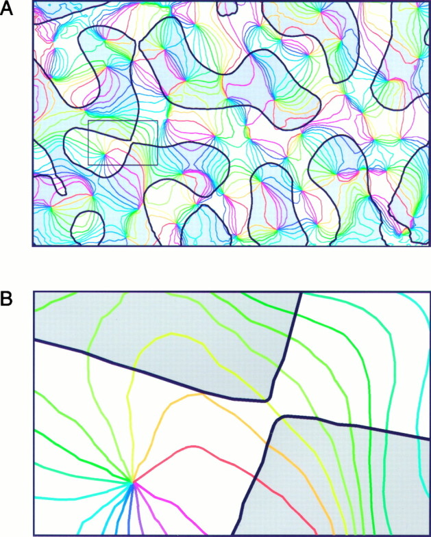
Relationship between ocular dominance and orientation maps. A, The colored iso-orientation lines were derived from the orientation preference map shown in Figure 2. All points on lines with a given color prefer the same orientation. The contours of the ocular dominance columns were obtained from the ocular dominance map of the same cortical region, using an objective automated procedure; gray denotes contralateral eye dominance. On closer inspection it becomes clear that both systems are spatially related: many iso-orientation lines cross the borders between ocular dominance columns close to right angles, and the pinwheel-centers are preferentially located in the middle of the ocular dominance columns.B, Enlarged detail from A (seesmall rectangle on the left side of the map), showing that the tendency for perpendicular intersections is maintained even in regions where the ocular dominance bands make sharp turns.

To quantify the geometric relationships between the orientation and ocular dominance maps we measured the angles between iso-orientation lines and ocular dominance column borders as described in Materials and Methods. It should be noted that the algorithm we used does not determine these angles only for the iso-orientation lines shown in Figure 4. To avoid a sampling bias attributable to the fact that only discrete iso-orientation lines are shown in this figure, we calculated the intersection angle for every point on the borders between ocular dominance columns. The distributions of these angles for maps imaged in three cats are shown in Figure 5. In all cases there is a clear shift toward right angles. One might argue that because of simple geometric reasons a higher proportion of right angles is always to be expected when the relationship between a circular pattern (the radially arranged orientation domains) and a linear pattern (the ocular dominance columns) is analyzed. One straightforward way to test this is to analyze the relationship between maps originating from different animals, that is, to overlay an orientation map from one cat with an ocular dominance map from another cat (Fig. 5,gray histograms). As can be seen, in these control cases the distribution of the intersection angles is essentially flat. The mean of the average angle for all cats from which we obtained ocular dominance columns was 51.7 ± 0.8° (n = 6), whereas in the control cases it was 45.8 ± 1.2° (n = 6) (p < 0.05; Wilcoxon signed-rank test), a value that comes very close to the expected average angle of 45°.

Fig. 5.

Quantitative analysis of intersection angles between iso-orientation lines and ocular dominance borders. Nine histograms are shown in the form of a 3 × 3 matrix. The black histograms along the diagonal show the distribution of intersection angles from three cats. In all cases there is a clear predominance of large intersection angles. Each of the gray histogramsoff the diagonal was computed by overlaying an orientation map from one cat with an ocular dominance map from a different cat. In these control cases the distributions are nearly flat.

To verify our observation that the pinwheel-centers are preferentially located in the middle of ocular dominance columns we first applied a search algorithm to find the pinwheel-centers. Next we determined the center regions of the ocular dominance columns: those 10% of the pixels in an ocular dominance map with the highest values were defined as corresponding to the centers of the columns of one eye, whereas the 10% with the lowest pixel values defined the centers of the columns of the other eye. Thus, the combined center regions made up 20% of the area of an ocular dominance map. Accordingly, the border regions were defined as 20% of the area of a map with intermediate pixel values. Analysis of our maps (n = 6) in this way revealed a steady decline in pinwheel-center density when moving from the central regions of the ocular dominance columns toward their borders (Fig.6). The total number of pinwheel-centers found in the central 20% of the ocular dominance maps is significantly higher than the value one would expect if the pinwheel-centers were distributed randomly (p < 0.01; χ² test).

Fig. 6.

Relative frequency of pinwheel-centers in different subregions of ocular dominance maps. The maps (n = 6) were divided into five regions of equal area, with the 0–20 percentile denoting the center and the 80–100 percentile denoting the border regions of the ocular dominance columns (error bars are SEM). The dotted line indicates the expected value (20%) if the pinwheel-centers were distributed randomly. There is a high incidence of pinwheel-centers in the center regions of the ocular dominance columns.

In summary, we find that specific spatial relationships are present between the orientation and ocular dominance maps in cat area 17. The pinwheel-centers tend to lie in the middle of ocular dominance columns, and the iso-orientation lines that connect neighboring pinwheel-centers in adjacent ocular dominance columns often cross the borders between these columns at right angles.

Relationship between spatial frequency and orientation maps

Figure 7 shows two sets of iso-orientation maps obtained after binocular stimulation with different spatial frequencies. At each orientation the two maps of a pair have a rather similar layout overall, but they clearly differ in the exact size, shape, and position of the patches. This becomes evident if one compares, for instance, the outlines of the patches from the 90° low spatial frequency map (Fig. 7C) with the activated regions in the 90° high spatial frequency map (Fig.7G). The orientation preference and the spatial frequency map calculated from these iso-orientation maps are depicted in Figure8. As can be seen in the spatial frequency map in Figure 8B, there is an imbalance between the cortical regions preferring stimuli of low and high spatial frequencies that we noted in many experiments: the low spatial frequency domains (dark patches) seem to be embedded in a matrix of high spatial frequency preference. Figure9 shows the combined orientation and spatial frequency maps. Again, at first sight it seems rather difficult to find any obvious relationships between both maps. Although in many instances individual orientation columns consist of two regions, one preferring high and the other low spatial frequencies, there are also orientation columns that clearly stay confined to either a low or a high spatial frequency domain. To test whether both maps are spatially related, we therefore used the same quantitative analysis that was used for the ocular dominance and orientation maps. The distribution of the crossing angles between iso-orientation lines and the borders of spatial frequency domains are illustrated in Figure 10. A predominance of right angles becomes evident again, although the shift toward right angles is not as strong as for the ocular dominance columns. The average crossing angle was 49.7 ± 0.8° (n = 13) for orientation and spatial frequency maps from the same cat and 46.1 ± 0.8° (n = 13) in the control cases (p< 0.05; Wilcoxon signed-rank test).

Fig. 7.

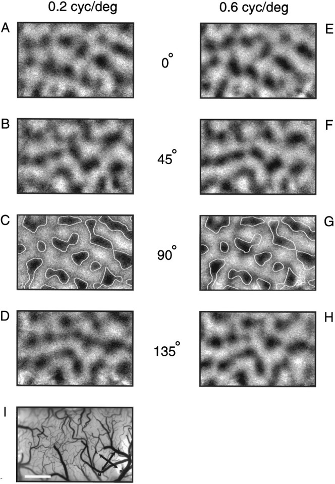
Stimulation with different spatial frequencies causes different activity patterns. A–H, Iso-orientation maps obtained after stimulation with oriented gratings at a low (0.2 cycles/degree) and a high (0.6 cycles/degree) spatial frequency. At a given orientation the low and high spatial frequency maps are similar, but not identical (see outlines from the map inC, copied to the map in G).I, Cortical blood vessel pattern. Scale bar, 1 mm.

Fig. 8.

Stimulus preference maps derived from the iso-orientation maps shown in Figure 7. A, Orientation preference map. B, Spatial frequency map. Dark patches were activated by low spatial frequencies, and lighter regions preferred high spatial frequencies. Note that the low spatial frequency patches tend to form islands in a matrix of high spatial frequency preference. Scale bar, 1 mm.  

Fig. 9.

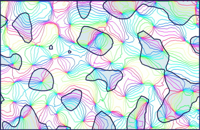
Relationship between spatial frequency and orientation maps. The iso-orientation lines and contours of the spatial frequency domains were obtained from the maps shown in Figure 8;gray regions preferred low spatial frequencies. Scrutiny of this image reveals that the iso-orientation lines tend to cross the borders between spatial frequency domains at right angles, and that the pinwheel-centers are often located in the centers of either low or high spatial frequency domains.

Fig. 10.

Intersection angles of iso-orientation lines with borders between spatial frequency domains. Nine histograms are shown in the form of a 3 × 3 matrix. The black histogramsalong the diagonal show the distribution of intersection angles from three kittens. Large angles (black histograms) are clearly over-represented, whereas this is not the case in the controls (gray histograms).

We also analyzed whether the locations of the pinwheel-centers are in any way correlated with the spatial frequency domains. Here too it turned out that the density of pinwheel-centers in the central regions of the spatial frequency domains is slightly but significantly higher than expected according to chance (Fig.11) (p < 0.05; χ² test).

Fig. 11.

Relative frequency of pinwheel-centers in different regions of spatial frequency maps (n = 13). Same conventions as in Figure 6. Pinwheel-centers are found more often in the center regions than near the borders of spatial frequency domains.

Relationship between ocular dominance and spatial frequency maps

Finally, we also analyzed whether a geometric relationship exists between the ocular dominance and the spatial frequency domains. This issue is of particular interest because we have found recently that the low spatial frequency domains in cat visual cortex correspond to the cytochrome oxidase blobs (Shoham et al., 1997). Therefore, information about the relationship between ocular dominance and spatial frequency domains relates to the question of whether the cytochrome oxidase blobs in cat visual cortex, as in the macaque monkey (Horton and Hubel, 1981), are centered on the ocular dominance columns. This problem has been investigated previously, with conflicting results (Dyck and Cynader, 1993; Murphy et al., 1995). Figure12 shows outlines of an ocular dominance map overlaid with outlines of a spatial frequency map. Although visual inspection of the maps did not reveal any apparent relationships, quantitative analysis proved that both systems are not independent of each other: there is a tendency for the low spatial frequency domains to preferentially lie in the centers of ocular dominance columns rather than on their borders. This tendency becomes evident when counting the centers of low spatial frequency domains near the borders between ocular dominance columns: on average only 4.1% of these centers are located in the border region of ocular dominance columns (defined as 20% of the total map area) (p < 0.05; χ² test;n = 6 maps) (Fig. 13). Thus, the low spatial frequency domains, and therefore the cytochrome oxidase blobs in cat visual cortex, seem to avoid the border regions of the ocular dominance columns.

Fig. 12.

Relationship between ocular dominance and spatial frequency domains. In this overlay contralateral eye dominance is coded by light gray with red outlines, and low spatial frequency is coded by dark gray withblack outlines. No obvious spatial relationships are discernible at a first glance. Quantitative analysis, however, reveals that the centers of low spatial frequency domains tend to avoid the borders of the ocular dominance columns (see Fig. 13).

Fig. 13.

Frequency of centers of low spatial frequency domains in different regions of ocular dominance maps (n = 6). Same conventions as in Figure 6. Only very few low spatial frequency domains (and thus blobs) are centered on the border regions of ocular dominance columns.

DISCUSSION

We performed most of our experiments on 8- to 12-week-old cats. Although cats of this age are still within the critical period (Hubel and Wiesel, 1970), ocular dominance columns of normally raised cats are adult-like at this age (LeVay et al., 1978), and the orientation system changes very little during this period (Gödecke et al., 1997). Finally, the spatial frequency tuning bandwidth reaches adult-like values at 6 weeks [although the best spatial frequencies in kittens are slightly shifted toward lower values (Derrington and Fuchs, 1981)]. We are therefore confident that the results described here also hold true for the fully matured visual cortex of cats.

Spatial relationships between columnar systems in the visual cortex

Orientation and ocular dominance

Hubel and Wiesel (1972, 1974, 1977) were the first to argue that a perpendicular relationship between orientation and ocular dominance columns might have advantages for visual information processing, yet 2-deoxyglucose studies seemed to indicate that this is not the case (Hubel et al., 1978; Löwel et al., 1988). However, as pointed out by Blasdel (1992), mapping of orientation columns with 2-deoxyglucose is not an adequate method to answer this question. Although this technique visualizes all regions of the cortex that respond to one particular orientation, it does not allow us to draw any firm conclusions about the complete layout of orientation preference in the cortex, and therefore it is difficult to analyze geometric relationships.

With the development of the optical imaging technique it became possible to visualize the complete orientation preference map (Blasdel and Salama, 1986; Grinvald et al., 1986). Experiments using this method have shown that orientation and ocular dominance columns in monkey striate cortex are spatially related in a specific way: pinwheel-centers tend to be centered on the ocular dominance columns, and iso-orientation lines often intersect borders between adjacent ocular dominance columns at right angles (Bartfeld and Grinvald, 1992; Obermayer and Blasdel, 1993; Blasdel et al., 1995). Our study demonstrates that despite the more irregular layout of ocular dominance in the cat, the very same spatial relationships govern the functional architecture in cat area 17. Our finding that specific geometric relationships are maintained even in regions of the cortex where the layout of ocular dominance columns is highly irregular indicates that whatever mechanism produces this specific mutual arrangement must act on a very local scale.

Orientation and spatial frequency

Only a few studies have examined the geometric relationship between orientation and spatial frequency maps. This is most likely caused by the fact that the concept of a columnar organization for spatial frequency, although demonstrated by Tootell and colleagues (1981), has never gained strong influence on ideas about the functional architecture of cat visual cortex. Maffei and co-workers (Maffei and Fiorentini, 1977; Berardi et al., 1982) found a relationship between spatial frequency and orientation preference of neighboring cells in cat visual cortex. However, it was based on the assumption that spatial frequency preference is arranged in layers. Although 2-deoxyglucose data (Tootell et al., 1981) and our own electrophysiological results (Shoham et al., 1997) make a layered arrangement unlikely, their observation that in tangential electrode penetrations systematic changes in orientation preference are accompanied by only minimal changes in optimum spatial frequency (Maffei and Fiorentini, 1977;Berardi et al., 1982) is compatible with our finding of acolumnar organization of both parameters together with a predominance of right angle crossings.

Ocular dominance and spatial frequency domains

In cat visual cortex the low spatial frequency domains coincide with the cytochrome oxidase blobs (Shoham et al., 1997). Therefore the question of geometric relationships between ocular dominance and spatial frequency domains is closely related to the spatial relation between blobs and ocular dominance columns. Dyck and Cynader (1993) examined this issue and did not detect any relationships, whereas Murphy et al. (1995) did report a relationship. Given the fact that also in our hands this relatively faint effect was demonstrable only with a quantitative analysis, it is not surprising that Dyck and Cynader (1993) did not detected the relationship. It seems reasonable to conclude from the three studies that there is a weak relationship between blobs (and therefore spatial frequency domains) and ocular dominance columns. Maybe more significant than the weak effect itself is the striking difference from macaque visual cortex, with its blobs nearly perfectly aligned on the ocular dominance columns (Hendrickson et al., 1981; Horton and Hubel, 1981; Horton, 1984).

Interestingly, a recent study on squirrel monkey visual cortex reported that the blobs in this species are not aligned with ocular dominance columns (Horton and Hocking, 1996a), indicating that differences in the relationship between blobs and ocular dominance columns do not simply reflect a dichotomy between primates and carnivores. Rather, the lack of clear relationships between blobs and ocular dominance columns in cats as well as squirrel monkeys might correlate with the rather weak mapping of one or both parameters in the visual cortex of these animals. Although squirrel monkeys have distinct cytochrome oxidase blobs (Horton, 1984), the segregation according to ocular dominance is not very pronounced in squirrel monkeys (Horton and Hocking, 1996a; Livingstone, 1996); conversely, cats have reasonably well defined ocular dominance columns but only faint blobs and relatively weak spatial frequency domains.

Functional significance of geometric relationships between columnar systems

A number of studies that examined relationships between columnar systems in other systems basically came to conclusions similar to ours (Bartfeld and Grinvald, 1992; Blasdel, 1992; Obermayer and Blasdel, 1993; Malonek et al., 1994; Blasdel et al., 1995; Shmuel and Grinvald, 1996; Weliky et al., 1996; Crair et al., 1997). The consistency of these findings suggests that spatial relationships between columnar systems are of functional significance for visual information processing.

The presence of columns in the visual cortex creates a sampling problem: each point in the visual world has to be analyzed with respect to all possible stimulus features. For the cortex to achieve a complete “coverage” (a term originally coined for the retina) (e.g.,Wässle and Boycott, 1991), all possible combinations of stimulus properties have to be represented in the cortical point image (i.e., the region of cortex analyzing inputs from any given point in the visual world) (Dow et al., 1981). Obviously, the best solution to this problem would be a “salt and pepper” mixing of cells with different response properties. However, response properties in the cortex are organized in a columnar, patchy manner. Therefore these columns have to be arranged in a specific way to ensure an optimal coverage (Hubel and Wiesel, 1974, 1977). One possible way to optimize coverage is to assign different periodicities to the different columnar systems (Swindale, 1991). However, many studies (e.g., Löwel, 1994; Horton and Hocking, 1996b) and our own data show that periodicities can change dramatically within areas as well as between animals, making it unlikely that differences in average periodicities are useful to optimize coverage. Geometric relationships between different types of columns are a different way to achieve optimal coverage. Intuitively, the tendency for right angle crossings seems to be an optimal solution, because this arrangement minimizes the cortical area containing all possible combinations of response properties. Formally, the goal of maximizing coverage is analogous to a dimension reduction problem, because the multidimensional stimulus space has to be mapped onto the two-dimensional surface of the cortex. Models based on different implementations of the dimension reduction approach produce maps that are very similar to the maps reported here (Obermayer et al., 1992;Erwin et al., 1995). In particular, the simulated maps show a preponderance of right angle crossings and a high incidence of pinwheel-centers in the middle of ocular dominance columns.

One problem concerning the demand for complete coverage arises from the fact that the cat’s visual cortex contains more than just the three columnar systems analyzed here. Among others, direction maps (Swindale et al., 1987; Shmuel and Grinvald, 1996) and on/off maps have been reported (Gordon et al., 1993) in cat visual cortex, and it seems likely that additional types of domains will be found in the future. With an increasing number of stimulus features being represented in a columnar manner, the number of possible permutations rises rapidly. Specific geometric arrangements such as those found here might therefore not suffice to maintain complete coverage.

It is important to note, however, that although a complete coverage is accomplished in the retina, the situation in the cortex is likely to be different: visual information is processed in parallel channels, which are at least partially segregated. This principle has been clearly demonstrated in primates (Livingstone and Hubel, 1988), and recent evidence suggests that it might be valid in nonprimates as well (Boyd and Matsubara, 1996; Hübener et al., 1996; Shoham et al., 1997). Thus, different aspects of the visual environment are analyzed in different compartments, which means in turn that not all possible combinations of stimulus parameters occur. Rather, certain combinations are actively excluded, as can be seen for example in macaque area V2, where cells selective for depth are usually not color sensitive and vice versa (Hubel and Livingstone, 1987). Given the multitude of columnar systems, complete coverage for all possible combinations of stimulus parameters seems impossible, and in fact it might not be realized in the visual cortex.

In summary then, we find that specific rules govern the geometric relationships between orientation, ocular dominance, and spatial frequency domains in cat primary visual cortex. These rules most likely ensure optimal coverage. However, they are not rigidly followed, and therefore the visual cortex cannot be considered a “crystalline” structure built from identical modules, but rather it is composed of “mosaics” of functional domains for the different properties that are arranged in a nonrandom manner.

REFERENCES

- 1.Anderson PA, Olavarria J, Van Sluyters RC. The overall pattern of ocular dominance bands in cat visual cortex. J Neurosci. 1988;8:2183–2200. doi: 10.1523/JNEUROSCI.08-06-02183.1988. [DOI] [PMC free article] [PubMed] [Google Scholar]
- 2.Bartfeld E, Grinvald A. Relationships between orientation preference pinwheels, cytochrome oxidase blobs and ocular dominance columns in primate striate cortex. Proc Natl Acad Sci USA. 1992;89:11905–11909. doi: 10.1073/pnas.89.24.11905. [DOI] [PMC free article] [PubMed] [Google Scholar]
- 3.Berardi N, Bisti S, Cattaneo A, Fiorentini A, Maffei L. Correlation between the preferred orientation and spatial frequency of neurones in visual areas 17 and 18 of the cat. J Physiol (Lond) 1982;323:603–618. doi: 10.1113/jphysiol.1982.sp014094. [DOI] [PMC free article] [PubMed] [Google Scholar]
- 4.Blasdel GG. Differential imaging of ocular dominance and orientation selectivity in monkey striate cortex. J Neurosci. 1992;12:3115–3138. doi: 10.1523/JNEUROSCI.12-08-03115.1992. [DOI] [PMC free article] [PubMed] [Google Scholar]
- 5.Blasdel GG, Salama G. Voltage-sensitive dyes reveal a modular organization in monkey striate cortex. Nature. 1986;321:579–585. doi: 10.1038/321579a0. [DOI] [PubMed] [Google Scholar]
- 6.Blasdel GG, Obermayer K, Kiorpes L. Organization of ocular dominance and orientation columns in the striate cortex of neonatal macaque monkeys. Vis Neurosci. 1995;12:589–603. doi: 10.1017/s0952523800008476. [DOI] [PubMed] [Google Scholar]
- 7.Bonhoeffer T, Grinvald A. Iso-orientation domains in cat visual cortex are arranged in pinwheel-like patterns. Nature. 1991;353:429–431. doi: 10.1038/353429a0. [DOI] [PubMed] [Google Scholar]
- 8.Bonhoeffer T, Grinvald A. The layout of iso-orientation domains in area 18 of cat visual cortex. Optical imaging reveals a pinwheel-like organization. J Neurosci. 1993;13:4157–4180. doi: 10.1523/JNEUROSCI.13-10-04157.1993. [DOI] [PMC free article] [PubMed] [Google Scholar]
- 9.Bonhoeffer T, Grinvald A. Optical imaging based on intrinsic signals: the methodology. In: Toga A, Mazziotta JC, editors. Brain mapping: the methods. Academic; San Diego: 1996. pp. 55–97. [Google Scholar]
- 10.Bonhoeffer T, Kim D-S, Malonek D, Shoham D, Grinvald A. Optical imaging of the layout of functional domains in Area 17 and across the Area 17/18 border in cat visual cortex. Eur J Neurosci. 1995;7:1973–1988. doi: 10.1111/j.1460-9568.1995.tb00720.x. [DOI] [PubMed] [Google Scholar]
- 11.Boyd JD, Matsubara JA. Laminar and columnar patterns of geniculocortical projections in the cat: relationship to cytochrome oxidase. J Comp Neurol. 1996;365:659–682. doi: 10.1002/(SICI)1096-9861(19960219)365:4<659::AID-CNE11>3.0.CO;2-C. [DOI] [PubMed] [Google Scholar]
- 12.Crair MC, Ruthazer ES, Gillespie DC, Stryker MP. Ocular dominance peaks at pinwheel center singularities of the orientation map in cat visual cortex. J Neurophysiol. 1997;77:3381–3385. doi: 10.1152/jn.1997.77.6.3381. [DOI] [PubMed] [Google Scholar]
- 13.Derrington AM, Fuchs AF. The development of spatial-frequency selectivity in kitten striate cortex. J Physiol (Lond) 1981;316:1–10. doi: 10.1113/jphysiol.1981.sp013767. [DOI] [PMC free article] [PubMed] [Google Scholar]
- 14.Dow BM, Snyder AZ, Vautin RG, Bauer R. Magnification factor and receptive field size in foveal striate cortex of the monkey. Exp Brain Res. 1981;44:213–228. doi: 10.1007/BF00237343. [DOI] [PubMed] [Google Scholar]
- 15.Dyck RH, Cynader MS. An interdigitated columnar mosaic of cytochrome oxidase, zinc, and neurotransmitter-related molecules in cat and monkey visual cortex. Proc Natl Acad Sci USA. 1993;90:9066–9069. doi: 10.1073/pnas.90.19.9066. [DOI] [PMC free article] [PubMed] [Google Scholar]
- 16.Erwin E, Obermayer K, Schulten K. Models of orientation and ocular dominance columns in the visual cortex: a critical comparison. Neural Comput. 1995;7:425–468. doi: 10.1162/neco.1995.7.3.425. [DOI] [PubMed] [Google Scholar]
- 17.Frostig RD, Lieke EE, Ts’o DY, Grinvald A. Cortical functional architecture and local coupling between neuronal activity and the microcirculation revealed by in vivo high-resolution optical imaging of intrinsic signals. Proc Natl Acad Sci USA. 1990;87:6082–6086. doi: 10.1073/pnas.87.16.6082. [DOI] [PMC free article] [PubMed] [Google Scholar]
- 18.Gödecke I, Kim DS, Bonhoeffer T, Singer W. Development of orientation preference maps in area 18 of kitten visual cortex. Eur J Neurosci. 1997;9:1754–1762. doi: 10.1111/j.1460-9568.1997.tb01533.x. [DOI] [PubMed] [Google Scholar]
- 19.Gordon JA, Ruthazer ES, Stryker MP. Segregation of on- and off-center afferents to cat visual cortex. Soc Neurosci Abstr. 1993;19:333. [Google Scholar]
- 20.Grinvald A, Lieke EE, Frostig RD, Gilbert CD, Wiesel TN. Functional architecture of cortex revealed by optical imaging of intrinsic signals. Nature. 1986;324:361–364. doi: 10.1038/324361a0. [DOI] [PubMed] [Google Scholar]
- 21.Hendrickson AE, Hunt SP, Wu J-Y. Immunocytochemical localization of glutamic acid decarboxylase in monkey striate cortex. Nature. 1981;292:605–607. doi: 10.1038/292605a0. [DOI] [PubMed] [Google Scholar]
- 22.Horton JC. Cytochrome oxidase patches: a new cytoarchitectonic feature of monkey visual cortex. Philos Trans R Soc Lond [Biol] 1984;304:199–253. doi: 10.1098/rstb.1984.0021. [DOI] [PubMed] [Google Scholar]
- 23.Horton JC, Hocking DR. Anatomical demonstration of ocular dominance columns in striate cortex of the squirrel monkey. J Neurosci. 1996a;16:5510–5522. doi: 10.1523/JNEUROSCI.16-17-05510.1996. [DOI] [PMC free article] [PubMed] [Google Scholar]
- 24.Horton JC, Hocking DR. Intrinsic variability of ocular dominance column periodicity in normal macaque monkeys. J Neurosci. 1996b;16:7228–7239. doi: 10.1523/JNEUROSCI.16-22-07228.1996. [DOI] [PMC free article] [PubMed] [Google Scholar]
- 25.Horton JC, Hubel DH. Regular patchy distribution of cytochrome oxidase staining in primary visual cortex of macaque monkey. Nature. 1981;292:762–764. doi: 10.1038/292762a0. [DOI] [PubMed] [Google Scholar]
- 26.Hubel DH, Livingstone MS. Segregation of form, color, and stereopsis in primate area 18. J Neurosci. 1987;7:3378–3415. doi: 10.1523/JNEUROSCI.07-11-03378.1987. [DOI] [PMC free article] [PubMed] [Google Scholar]
- 27.Hubel DH, Wiesel TN. Receptive fields, binocular interactions and functional architecture in the cat’s visual cortex. J Physiol (Lond) 1962;160:106–154. doi: 10.1113/jphysiol.1962.sp006837. [DOI] [PMC free article] [PubMed] [Google Scholar]
- 28.Hubel DH, Wiesel TN. Shape and arrangement of columns in cat’s striate cortex. J Physiol (Lond) 1963;165:559–568. doi: 10.1113/jphysiol.1963.sp007079. [DOI] [PMC free article] [PubMed] [Google Scholar]
- 29.Hubel DH, Wiesel TN. The period of susceptibility to the physiological effects of unilateral eye closure in kittens. J Physiol (Lond) 1970;206:419–436. doi: 10.1113/jphysiol.1970.sp009022. [DOI] [PMC free article] [PubMed] [Google Scholar]
- 30.Hubel DH, Wiesel TN. Laminar and columnar distribution of geniculo-cortical fibers in the macaque monkey. J Comp Neurol. 1972;146:421–450. doi: 10.1002/cne.901460402. [DOI] [PubMed] [Google Scholar]
- 31.Hubel DH, Wiesel TN. Uniformity of monkey striate cortex: a parallel relationship between field size, scatter, and magnification factor. J Comp Neurol. 1974;158:295–305. doi: 10.1002/cne.901580305. [DOI] [PubMed] [Google Scholar]
- 32.Hubel DH, Wiesel TN. Functional architecture of macaque monkey visual cortex (Ferrier Lecture). Proc R Soc Lond [Biol] 1977;198:1–59. doi: 10.1098/rspb.1977.0085. [DOI] [PubMed] [Google Scholar]
- 33.Hubel DH, Wiesel TN, Stryker MP. Anatomical demonstration of orientation columns in macaque monkey. J Comp Neurol. 1978;177:361–380. doi: 10.1002/cne.901770302. [DOI] [PubMed] [Google Scholar]
- 34.Hübener M, Shoham D, Grinvald A, Bonhoeffer T. Spatial frequency, ocular dominance, and orientation maps and their relationship in kitten visual cortex. Soc Neurosci Abstr. 1995;21:771. [Google Scholar]
- 35.Hübener M, Schulze S, Bonhoeffer T. Cytochrome-oxidase blobs in cat visual cortex coincide with low spatial frequency columns. Soc Neurosci Abstr. 1996;22:951. [Google Scholar]
- 36.LeVay S, Voigt T. Ocular dominance and disparity coding in cat visual cortex. Vis Neurosci. 1988;1:395–414. doi: 10.1017/s0952523800004168. [DOI] [PubMed] [Google Scholar]
- 37.LeVay S, Stryker MP, Shatz CJ. Ocular dominance columns and their development in layer IV of the cat’s visual cortex: a quantitative study. J Comp Neurol. 1978;179:223–244. doi: 10.1002/cne.901790113. [DOI] [PubMed] [Google Scholar]
- 38.Livingstone MS. Ocular dominance columns in new world monkeys. J Neurosci. 1996;16:2086–2096. doi: 10.1523/JNEUROSCI.16-06-02086.1996. [DOI] [PMC free article] [PubMed] [Google Scholar]
- 39.Livingstone MS, Hubel DH. Anatomy and physiology of a color system in the primate visual cortex. J Neurosci. 1984;4:309–356. doi: 10.1523/JNEUROSCI.04-01-00309.1984. [DOI] [PMC free article] [PubMed] [Google Scholar]
- 40.Livingstone MS, Hubel DH. Segregation of form, color, movement, and depth: anatomy, physiology, and perception. Science. 1988;240:740–749. doi: 10.1126/science.3283936. [DOI] [PubMed] [Google Scholar]
- 41.Löwel S. Ocular dominance column development: strabismus changes the spacing of adjacent columns in cat visual cortex. J Neurosci. 1994;14:7451–7468. doi: 10.1523/JNEUROSCI.14-12-07451.1994. [DOI] [PMC free article] [PubMed] [Google Scholar]
- 42.Löwel S, Singer W. The pattern of ocular dominance columns in flat-mounts of the cat visual cortex. Exp Brain Res. 1987;68:661–666. doi: 10.1007/BF00249809. [DOI] [PubMed] [Google Scholar]
- 43.Löwel S, Bischof H-J, Leutenecker B, Singer W. Topographic relations between ocular dominance and orientation columns in the cat striate cortex. Exp Brain Res. 1988;71:33–46. doi: 10.1007/BF00247520. [DOI] [PubMed] [Google Scholar]
- 44.Maffei L, Fiorentini A. Spatial frequency rows in the striate visual cortex. Vision Res. 1977;17:257–264. doi: 10.1016/0042-6989(77)90089-x. [DOI] [PubMed] [Google Scholar]
- 45.Malonek D, Tootell RBH, Grinvald A. Optical imaging reveals the functional architecture of neurons processing shape and motion in owl monkey area MT. Proc R Soc Lond [Biol] 1994;258:109–119. doi: 10.1098/rspb.1994.0150. [DOI] [PubMed] [Google Scholar]
- 46.McConnell SK, LeVay S. Segregation of on- and off-center afferents in mink visual cortex. Proc Natl Acad Sci USA. 1984;81:1590–1593. doi: 10.1073/pnas.81.5.1590. [DOI] [PMC free article] [PubMed] [Google Scholar]
- 47.Murphy KM, Jones DG, Van Sluyters RC. Cytochrome-oxidase blobs in cat primary visual cortex. J Neurosci. 1995;15:4196–4208. doi: 10.1523/JNEUROSCI.15-06-04196.1995. [DOI] [PMC free article] [PubMed] [Google Scholar]
- 48.Obermayer K, Blasdel GG. Geometry of orientation and ocular dominance columns in monkey striate cortex. J Neurosci. 1993;13:4114–4129. doi: 10.1523/JNEUROSCI.13-10-04114.1993. [DOI] [PMC free article] [PubMed] [Google Scholar]
- 49.Obermayer K, Blasdel GG, Schulten K. Statistical-mechanical analysis of self-organization and pattern formation during the development of visual maps. Physical Rev. 1992;45:7568–7589. doi: 10.1103/physreva.45.7568. [DOI] [PubMed] [Google Scholar]
- 50.Payne BR, Berman NEJ, Murphy EH. Organization of direction preferences in cat visual cortex. Brain Res. 1981;211:445–450. doi: 10.1016/0006-8993(81)90971-9. [DOI] [PubMed] [Google Scholar]
- 51.Ratzlaff EH, Grinvald A. A tandem-lens epifluorescence macroscope: hundred-fold brightness advantage for wide-field imaging. J Neurosci Methods. 1991;36:127–137. doi: 10.1016/0165-0270(91)90038-2. [DOI] [PubMed] [Google Scholar]
- 52.Shatz CJ, Stryker MP. Ocular dominance in layer IV of the cat’s visual cortex and the effects of monocular deprivation. J Physiol (Lond) 1978;281:267–283. doi: 10.1113/jphysiol.1978.sp012421. [DOI] [PMC free article] [PubMed] [Google Scholar]
- 53.Shatz CJ, Lindström S, Wiesel TN. The distribution of afferents representing the right and left eyes in the cat’s visual cortex. Brain Res. 1977;131:103–116. doi: 10.1016/0006-8993(77)90031-2. [DOI] [PubMed] [Google Scholar]
- 54.Shmuel A, Grinvald A. Functional organization for direction of motion and its relationship to orientation maps in cat area 18. J Neurosci. 1996;16:6945–6964. doi: 10.1523/JNEUROSCI.16-21-06945.1996. [DOI] [PMC free article] [PubMed] [Google Scholar]
- 55.Shoham D, Hübener M, Bonhoeffer T, Grinvald A. Spatiotemporal frequency columns in cat visual cortex. Isr J Med Sci. 1995;31:752. [Google Scholar]
- 56.Shoham D, Hübener M, Schulze S, Grinvald A, Bonhoeffer T. Spatio-temporal frequency domains and their relation to cytochrome oxidase staining in cat visual cortex. Nature. 1997;385:529–533. doi: 10.1038/385529a0. [DOI] [PubMed] [Google Scholar]
- 57.Swindale NV. Coverage and the design of striate cortex. Biol Cybern. 1991;65:415–424. doi: 10.1007/BF00204654. [DOI] [PubMed] [Google Scholar]
- 58.Swindale NV, Matsubara JA, Cynader MS. Surface organization of orientation and direction selectivity in cat area 18. J Neurosci. 1987;7:1414–1427. doi: 10.1523/JNEUROSCI.07-05-01414.1987. [DOI] [PMC free article] [PubMed] [Google Scholar]
- 59.Tolhurst DJ, Dean AF, Thompson ID. Preferred direction of movement as an element in the organization of cat visual cortex. Exp Brain Res. 1981;44:340–342. doi: 10.1007/BF00236573. [DOI] [PubMed] [Google Scholar]
- 60.Tootell RBH, Silverman MS, De Valois RL. Spatial frequency columns in primary visual cortex. Science. 1981;214:813–815. doi: 10.1126/science.7292014. [DOI] [PubMed] [Google Scholar]
- 61.Tootell RBH, Silverman MS, Hamilton SL, Switkes E, De Valois RL. Functional anatomy of macaque striate cortex. V. Spatial frequency. J Neurosci. 1988;8:1610–1624. doi: 10.1523/JNEUROSCI.08-05-01610.1988. [DOI] [PMC free article] [PubMed] [Google Scholar]
- 62.Ts’o DY, Frostig RD, Lieke EE, Grinvald A. Functional organization of primate visual cortex revealed by high resolution optical imaging. Science. 1990;249:417–420. doi: 10.1126/science.2165630. [DOI] [PubMed] [Google Scholar]
- 63.Wässle H, Boycott BB. Functional architecture of the mammalian retina. Physiol Rev. 1991;71:447–480. doi: 10.1152/physrev.1991.71.2.447. [DOI] [PubMed] [Google Scholar]
- 64.Weliky M, Bosking WH, Fitzpatrick D. A systematic map of direction preference in primary visual cortex. Nature. 1996;379:725–728. doi: 10.1038/379725a0. [DOI] [PubMed] [Google Scholar]
- 65.Zahs KR, Stryker MP. Segregation of on and off afferents to ferret visual cortex. J Neurophysiol. 1988;59:1410–1429. doi: 10.1152/jn.1988.59.5.1410. [DOI] [PubMed] [Google Scholar]