Neural Delays Shape Selectivity to Interaural Intensity Differences in the Lateral Superior Olive

Abstract

Neurons in the lateral superior olive (LSO) respond selectively to interaural intensity differences (IIDs), one of the chief cues used to localize sounds in space. LSO cells are innervated in a characteristic pattern: they receive an excitatory input from the ipsilateral ear and an inhibitory input from the contralateral ear. Consistent with this pattern, LSO cells generally are excited by sounds that are more intense at the ipsilateral ear and inhibited by sounds that are more intense at the contralateral ear. Despite their relatively homogeneous pattern of innervation, IID selectivity varies substantially from cell to cell, such that selectivities are distributed over the range of IIDs that would be encountered in nature. For some time, researchers have speculated that the relative timing of the excitatory and inhibitory inputs to an LSO cell might shape IID selectivity. To test this hypothesis, we recorded from 50 LSO cells in the free-tailed bat while presenting stimuli that varied in interaural intensity and in interaural time of arrival. The results suggest that, for more than half of the cells, the latency of inhibition was several hundred microseconds longer than the latency of excitation. Increasing the intensity to the inhibitory ear shortened the latency of inhibition and brought the timing of the inputs from the two ears into register. Thus, a neural delay of the inhibition helped to define the IID selectivity of these cells, accounting for a significant part of the variation in selectivity among LSO cells.

Interaural intensity differences (IIDs) are the binaural cues that animals use to localize high frequency sounds (Erulkar, 1972; Irvine, 1992). In mammals, IIDs are first coded in the lateral superior olive (LSO). LSO cells receive excitatory inputs from the ipsilateral ear and inhibitory inputs from the contralateral ear, and they code IIDs by subtracting the activity of the inhibitory input from that of the excitatory input (Boudreau and Tsuchitani, 1968; Caird and Klinke, 1983; Sanes and Rubel, 1988; Covey et al., 1991). The particular IID that results in a criterion degree of inhibition varies among cells, which is a key factor that allows the population of cells to code for a variety of interaural intensity differences that correspond to different azimuthal locations.

Several researchers have proposed that the relative timing of the inputs from the two ears might play a role in shaping IID selectivity among LSO cells (Jeffress, 1948; Pollak, 1988; Tsuchitani, 1988; Irvine et al., 1995; Joris and Yin, 1995). The so-called latency hypothesis is based on two key features: (1) the relative arrival times of the inputs from the two ears differ among cells, and (2) changes in the relative intensity of the stimuli at the ears can shift the latencies of the inputs, affecting their coincidence. Yin and his colleagues (1985) have constructed a model of this second feature that we use here to illustrate the latency hypothesis (see Fig. 1). The graphs at the top of Figure 1 represent IID functions from two hypothetical cells differing in IID selectivity. The drawings at the bottom represent the excitatory and inhibitory postsynaptic potentials (EPSPs and IPSPs) evoked by different IIDs.

Fig. 1.

Model of the latency hypothesis. Top, Two IID functions from hypothetical LSO neurons illustrate different IID selectivities. Note that, compared with Cell A, Cell B responds to a wider range of IIDs. In other words, higher intensities at the inhibitory ear (more negative IIDs) are required to inhibit Cell B. Bottom, Hypothetical EPSPs and IPSPs show how the relative timing of excitation and inhibition could interact to generate different IID selectivities. In the situation shown here, IIDs from +20 to −10 dB are generated by holding the intensity to the ipsilateral (excitatory) ear constant at 40 dB SPL and varying the intensity to the contralateral (inhibitory) ear from 20 to 50 dB SPL. Theupward-deflecting curves represent excitatory postsynaptic potentials (EPSPs), whereas the downward-deflecting curvesrepresent inhibitory postsynaptic potentials (IPSPs). Bars beneath EPSP curves indicate when spikes can be evoked. For both cells, increasing the intensity to the inhibitory ear causes the latency of the IPSP to shorten, its duration to lengthen, and its strength to increase. Cell A and Cell B differ in terms of the relative timing of excitation and inhibition, and the discrepancy helps to define which IIDs can evoke spikes and which cannot (i.e., IID selectivity).

The model shows how increasing the intensity at the inhibitory ear (i.e., changing the IID from +20 to −10 dB) causes the latency of the inhibitory input to shorten in both cells. For Cell A, the timing of the excitatory and inhibitory inputs is equal when the intensity at the two ears is equal (IID of 0 dB) and, consequently, the cell is silenced. A lower intensity at the inhibitory ear (IID of +10 dB) causes the inhibitory input to arrive later than the excitatory input, allowing the cell to respond. Conversely, a higher intensity at the inhibitory ear (IID of −10 dB) causes the inhibitory input to arrive earlier than the excitatory input, suppressing responses (assuming that the inhibition is longer-lasting than the excitation). For Cell B, the inhibitory input arrives later than the excitatory input when the intensities at both ears are equal. Hence, the stimulus at the inhibitory ear must be more intense to bring the inputs into register and silence the cell.

Brain slice studies support several aspects of the model in that increasing the stimulus voltage to the inhibitory pathway decreased the latency and lengthened the duration of IPSP for LSO cells (Sanes, 1990;Wu and Kelly, 1992). The appeal and strength of the model is that it is testable by electronically manipulating the timing and intensity of the signals to the ears, which is the technique we used to assess the role of neural delays in shaping IID selectivity in LSO cells.

MATERIALS AND METHODS

Surgical and recording procedures. Seven Mexican free-tailed bats, Tadarida brasiliensis mexicana, were experimental subjects. Before surgery, animals were anesthetized with methoxyflurane inhalation, and 15 mg/kg sodium pentobarbital was injected subcutaneously. The hair on the bat’s head was removed with a depilatory, and the head was secured in a head holder with a bite bar. The muscles and skin overlying the skull were reflected, and Xylocaine (Astra Chemical, Wedel, Germany) was applied topically to all open wounds. The surface of the skull was cleared of tissue, and a ground electrode was placed just beneath the skull over the posterior cerebellum. A layer of small glass beads and dental acrylic was placed on the surface of the skull to secure the ground electrode and to serve as a foundation layer to be used later for securing a metal rod to the bat’s head.

The bat was transferred to a heated (27–30°C), sound-attenuated room, where it was placed in a restraining apparatus attached to a custom-made stereotaxic instrument (Schuller et al., 1986). A small metal rod was cemented to the foundation layer on the skull and then attached to a bar mounted on the stereotaxic instrument to ensure uniform positioning of the head. A small hole (∼0.5–1.0 mm diameter) was then cut over the inferior colliculus on one side. Position of the hole and positioning of the electrode followed procedures described bySchuller et al. (1986). Recordings were begun after the bat was awake. If the animal struggled or otherwise seemed in discomfort, the local anesthetic was refreshed, and an additional subanesthetic injection of sodium pentobarbital (10 mg/kg body weight) was given subcutaneously. This dosage of pentobarbital never induced anesthesia: the bats were still awake in that their eyes were open, they drank water when it was administered, and they responded when we gently touched their face or ears. We did not notice any systematic changes in neuronal response properties from the pentobarbital. We administered the pentobarbital on only several occasions and then only once during a given recording session. Recording sessions generally lasted from 3 to 5 hr per day to minimize the animals’ discomfort from being restrained.

Action potentials were recorded with a glass pipette filled with buffered 1m NaCl. Electrode impedance ranged from 5–20 MΩ. Electrode penetrations were made vertically through the exposed dorsal surface of the inferior colliculus. Subsequently, the electrode was advanced from outside of the experimental chamber with a piezoelectric microdrive.

At the end of each experiment, the locations of recording sites were confirmed by a small iontophoretic injection of horseradish peroxidase (HRP). In each case recordings through the HRP electrode confirmed that the tip of the electrode was in a region dominated by IE cells. At 24 hr after the injection, the bat was deeply anesthetized and perfused through the heart with buffered saline and glutaraldehyde. The brain was dissected out, frozen, and cut into 40 μm sections, which were then processed for HRP reaction product. In each case the HRP deposit was located within the LSO. We emphasize that there is no guarantee that HRP deposit sites correspond precisely to recording sites, because we usually used different, steriotactically placed electrodes for HRP and for recording. However, given that limitation, it was reassuring that the HRP sites were consistent with the physiological results.

Acoustic stimuli and data acquisition. Pure tones with a duration of 50 msec were used as search stimuli. When a unit was encountered, its characteristic frequency and absolute threshold were audiovisually determined to set stimulus parameters subsequently controlled by computer. The characteristic frequency was defined as the frequency that elicited responses at the lowest sound intensity to which the unit was sensitive. Then binaural stimuli were presented to determine whether the unit was monaural or binaural and, if it was binaural, whether it was inhibitory/excitatory (IE) or excitatory/excitatory (EE). Units were classified as IE if sound at the contralateral (inhibitory) ear suppressed the responses evoked by the ipsilateral (excitatory) ear.

Stimuli used to investigate ITD and IID sensitivity were 2 msec downward frequency-modulated (FM) sweeps with a rise–fall time of 0.2 msec. The frequency of FM stimuli swept down from 5 kHz above to 5 kHz below the characteristic frequency of a unit. The FM sweeps at both ears were coherent in that they had the same frequency range and duration, and each began and ended with the same phase. The stimuli were presented via Brüel and Kjaer 0.635 cm microphones used as earphones fitted with probe tubes (5 mm diameter) that were placed in the funnel of each pinna. Maximum sound intensity was 90 dB sound pressure level (SPL) measured 0.5 cm from the opening of the probe tubes. Sound pressure and the frequency response of each earphone were measured with a 0.635 cm Brüel and Kjaer microphone. Each earphone showed less than <±3 dB variability for the frequency range usually used (15–80 kHz), and intensities between the earphones did not vary more than >±3 dB at any of those frequencies. Stimuli were presented at a rate of 4/sec. Acoustic isolation between the ears was better than 40 dB and was determined empirically by testing monaural units during the course of the experiments. A comparison of evoked responses to earphone stimulation transmitted through a coupling tube with those of free-field stimulation showed that free-field sound pressure level and calibrated level of the earphones corresponded exactly in their effectiveness to elicit evoked responses (Schlegel, 1977). For fundamentals between 10–50 kHz and 74 dB SPL (the highest intensity we used), all harmonics were at least 35 dB less intense than the fundamental. For higher frequencies, the harmonics were even lower.

A matrix of responses to different IIDs and ITDs was generated for each cell. ITDs were computer-controlled and varied in 100 μsec steps, usually ranging over ±1000 μsec. These ITDs are larger than the ITDs the animal would normally experience and are used here as a tool to evaluate the role of coincidence in shaping IID sensitivity. IIDs were generated by holding the intensity at the ipsilateral (excitatory) ear constant at about 20 dB above the threshold of a unit and varying the intensity at the contralateral (inhibitory) ear in 5 dB steps ranging from ∼30 below to 30 dB above the intensity at the excitatory ear. Each combination of IID and ITD was presented 10 times.

Only well isolated spikes were studied. Spikes were fed to a window discriminator, and the output of the discriminator was fed to the computer. Data were displayed on the computer screen for inspection during the experiments and stored on hard disk for later analysis with software programmed by M. Baumann and S. Kieslich (Sonderforschungsbereich 204, Germany).

RESULTS

Here we report on 50 neurons recorded from the LSO of the Mexican free-tailed bat. All of the cells responded to FM sweeps presented to the excitatory ear with 1–2 spikes per stimulus. The mean latency of the response to the 2 msec FM sweeps 20 dB above threshold was 5.6 msec and ranged from 3.2 to 8.5 msec. All units were excited by stimulation of the ipsilateral ear and inhibited by stimulation of the contralateral ear (IE type of neuron). We hereafter refer to the ipsilateral ear as the excitatory ear and the contralateral ear as the inhibitory ear. Interaural intensity difference (IID) functions were measured for each cell by driving the neuron with a fixed intensity at the excitatory ear and then documenting the suppressive influence of increasing intensities at the inhibitory ear. Because the intensity at the excitatory ear was fixed, each intensity at the inhibitory ear generated a different IID. By convention, positive IIDs indicate that the sound was more intense at the excitatory ear. The characteristic frequencies (the frequency to which the unit was most sensitive) ranged from 8 to 75 kHz.

Below, we first show that IID functions varied considerably among the cells sampled. We then show how changing the relative timing and intensity of the stimulus to the ears affected IID selectivity. Finally, we describe how 27 of the cells (54%) showed a neural delay of their inhibitory input relative to their excitatory input, which shaped IID selectivity as predicted by the latency hypothesis.

IID selectivity varied among LSO cells

Each of the 50 LSO cells showed a steep decline in spike count with increasing intensities at the inhibitory ear until spike activity was completely inhibited. Figure 2 (top) shows IID functions from six representative LSO cells. Although the general shape of the functions was similar among cells, responsiveness to specific IIDs varied considerably from cell to cell. For example, some cells were already completely inhibited when the intensity at the excitatory ear was greater than the intensity at the inhibitory ear (positive IIDs), and other cells were inhibited completely only when the intensity at the inhibitory ear was greater than the intensity at the excitatory ear (negative IIDs).

Fig. 2.

Representative IID functions and distribution of IIDs of complete inhibition for the 50 LSO neurons tested.Top, The IID functions from six cells illustrate how IID selectivity varied among the population from which we recorded. The IID of complete inhibition is indicated on one function. Bottom, Distribution of IIDs of complete inhibition for the 50 cells tested. Stimuli were 2 msec long, 10 kHz downward frequency sweeps centered at the characteristic frequency of each unit. The intensity to the ipsilateral (excitatory) ear was fixed at 20 dB above threshold, whereas the intensity to the contralateral (inhibitory) ear was varied.

The IID of complete inhibition was selected to characterize the IID function of each cell, because it distinguishes IIDs that evoke responses from those that do not. The histogram in Figure 2(bottom) shows the distribution of the IID of complete inhibition for the 50 cells tested. IIDs of complete inhibition ranged from +20 (excitatory ear more intense) to −40 dB (inhibitory ear more intense). This range of IID selectivities corresponds well with the range of IIDs that this species would normally encounter in the free field (Pollak, 1988).

IID selectivity was affected by interaural time differences

Changing the relative timing of the stimulus to the ears affected the way in which LSO cells responded to IIDs. These effects can be depicted in a two-dimensional matrix showing how a cell responded to different combinations of ITDs and IIDs. Figure 3 shows such a matrix, made up of dot rasters, for one representative LSO cell. Within each row of the matrix, IIDs change from +35 to +5 dB, all favoring the excitatory ear. Responses to these IIDs were measured for 21 experimentally induced interaural time differences (21 rows) in 100 μsec steps from +1000 (inhibitory ear leading) to −1000 μsec (excitatory ear leading).

Fig. 3.

Matrix of dot raster displays and selected IID and ITD functions from one LSO neuron. The matrix shows dot raster displays generated by 147 different combinations of IID and ITD. On they-axis, negative ITDs indicate that the signal to the contralateral (inhibitory) ear was delayed electronically relative to the signal to the ipsilateral (excitatory) ear, whereas positive ITDs indicate that the signal to the inhibitory ear was advanced. On thex-axis, decreasing IIDs correspond to greater intensities at the inhibitory ear. Each raster display in the matrix shows the responses to 10 presentations of the frequency sweep at one particular IID and ITD combination. The scale bar indicates the time frame for each raster display in the matrix. The characteristic frequency of this cell was 36.0 kHz, and the intensity at the excitatory ear was held constant at 50 dB SPL (20 dB above threshold). Note that the ITDs we selected to examine the timing of the neural inputs to the cell were much larger than the ITDs that the free-tailed bat would normally encounter in the free field. The small graphs show IID (A–C) and ITD (D–G) functions constructed from the spike counts along selected rows and columns of the matrix.

For the example in Figure 3, the inhibitory input was most effective at and near simultaneous stimulation of both ears (0 μsec,y-axis). In this unit, inhibition was already complete when the excitatory signal was 20 dB more intense than the inhibitory signal (+20 dB IID, x-axis). When the inhibitory signal was shifted in time in either direction, its effectiveness decreased and spikes recurred (vertical column at +20 dB IID). This effect is shown graphically by the V-shaped ITD function in Figure 3D(derived from the spike counts along the vertical column of the matrix at +20 dB IID).

The decrease in the inhibitory effect from time shifting the inhibitory signal could be compensated by increasing the inhibitory intensity. For example, the matrix of dot displays shows that when the inhibitory signal was delayed −300 μsec the intensity at the inhibitory ear had to be increased 10 dB (to an IID of +10 dB) to achieve a complete inhibition. The effect of increasing intensity at the inhibitory ear was to increase the range of ITDs at which complete inhibition was achieved. This can be seen in the matrix as an expansion of the ITDs that produce complete inhibition as the intensity to the inhibitory ear was increased, changing the IID from +20 to +5 dB. It is also illustrated in the four ITD functions below the matrix. Those functions changed from a V shape when the IID was +20 dB to progressively broader U shapes when the inhibitory intensity was increased to generate less positive IIDs. The significance of this broadening is considered in a later section.

The three functions to the right of the matrix show how time-shifting the signal to the inhibitory ear changed the IID function of the cell. Each curve was measured with a fixed interaural time difference, and the IID of complete inhibition is indicated by an arrow. When the stimulus was presented to both ears at the same time (Fig.3B), complete inhibition of spikes occurred at an IID of +20 dB. When the signal to the inhibitory ear was electronically advanced (Fig. 3A) or delayed (Fig. 3C) by 400 μsec, the inhibitory signal was still capable of completely inhibiting spike activity. However, in both cases the intensity at the inhibitory ear had to be increased, shifting the IID of complete inhibition to less positive values.

All cells showed time–intensity trading

In this section we describe in more detail the effects of delaying the signal to the inhibitory ear relative to the signal at the excitatory ear. As described above, when the signal at the inhibitory ear was delayed, greater intensities were required at the inhibitory ear to produce an equivalent degree of spike suppression, as compared with the intensity required with no delay. Hence, delaying the signal to the inhibitory ear caused the IID function of each cell to shift to a more negative IID of complete inhibition.

The shifts in IID functions that resulted from delaying the inhibitory signal varied in degree from cell to cell. Three examples are presented in Figure 4. The IID function of Cell A showed a relatively small shift when the signal to the inhibitory ear was delayed by −600 μsec. A greater shift was produced for Cell B when a delay of −800 μsec was used, and an even greater shift resulted from a delay of −600 μsec in Cell C. We point out that each of the shifted IID functions shown in Figure 5 represents the greatest shift documented for each cell. Shorter delays produced smaller shifts, but with larger delays, the cells could not be completely inhibited.

Fig. 4.

IID functions from three LSO cells illustrating how electronically delaying the signal to the inhibitory ear affected IID selectivity. Each graph shows the IID function of a cell when the stimulus was presented simultaneously at both ears (solid lines) and when the signal to the inhibitory ear was electronically delayed by 600 or 800 μsec relative to the signal to the excitatory ear (dashed lines). Arrows belowthe graphs indicate the magnitude of the shift for each cell. The characteristic frequencies of these cells included the following: Cell A, 49.3; Cell B, 45.0; and Cell C, 29.7 kHz; the intensity at the excitatory ear was held constant at 20 dB above threshold for each cell.

Fig. 5.

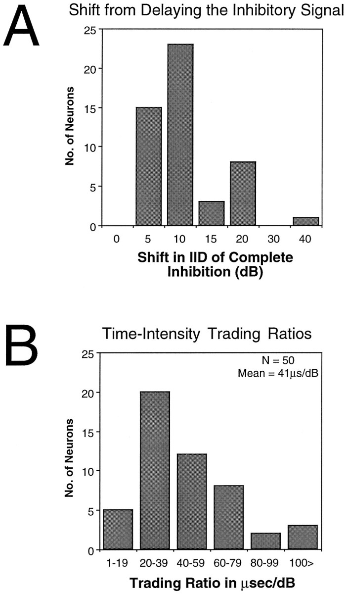
Effects of delaying the signal to the inhibitory ear on the IID of complete inhibition for the 50 LSO units tested.A, Distribution of shifts in the IID of complete inhibition.B, Distribution of time–intensity trading ratios for the 50 cells. All measures were made with the intensity at the excitatory ear fixed at 20 dB above threshold.

The IID of complete inhibition was used to quantify shifts in the IID functions. For Cell A in Figure 4, the IID of complete inhibition shifted by 5 dB, whereas it shifted by 10 dB for Cell B and 15 dB for Cell C. The bar graph in Figure 5A shows the distribution of shifts for the 50 cells tested. On average, the IID of complete inhibition shifted by 11 dB for a mean ITD shift of 450 μsec.

To quantify the relationship between time and intensity, the ratio of change in time over change in intensity was calculated for each cell. Applying this calculation to the cells in Figure 4 shows that the time–intensity ratios were quite variable from cell to cell. For Cell A, a delay of 600 μsec produced a shift of 5 dB, yielding a time–intensity ratio of 120 μsec per dB. The time–intensity ratio for Cell B was 80 μsec per dB, and the ratio for Cell C was 40 μsec per dB. The distribution of ratio values for the 50 cells tested is shown in Figure 5B. The average time–intensity ratio for the population was 41 μsec per dB. Hence, the IIDs that these animals would experience in the real world should substantially affect the latencies of excitation and inhibition, which is consistent with the assumptions of the latency hypothesis.

IID selectivity in half of the neurons was shaped by mismatches of excitatory and inhibitory latencies

In the previous section we focused on the effects of electronically delaying the signal to the inhibitory ear. In this section we will focus on the effects of advancing the signal to the inhibitory ear. This was the most crucial manipulation for testing the viability of the latency hypothesis. The latency hypothesis predicts that if the inhibitory latency is longer than the latency for excitation in a given cell, then the mismatch in latencies will influence the IID of complete inhibition of that cell. We tested for this type of latency mismatch and its effect on IID selectivity by advancing the signal to the inhibitory ear. We assumed that if inhibition was delayed relative to excitation, then we should be able to compensate for the latency mismatch by electronically advancing the inhibitory signal, and we should be able to see an effect in the spike counts. As described below, we found that, for approximately half of the cells, the latency of inhibition was longer than the latency of excitation and that the mismatch in timing affected IID selectivity in these cells, as predicted by the latency hypothesis.

To clarify the predictions of the latency hypothesis, we begin by considering a hypothetical LSO cell, the excitatory and inhibitory latencies of which are well matched at the IID of complete inhibition. Figure 6IA (left panel) shows the hypothetical EPSPs and IPSPs of such a cell. At the IID of complete inhibition, the strengths of excitation and inhibition are, by definition, matched. The important feature in this example is that the latencies of excitation and inhibition are also matched at this IID. For convenience, we refer to cells like this as “neurons with matched latencies,” meaning that the excitation and the inhibition arrive coincidentally at the LSO target cell when the strengths of excitation and inhibition are equal.

Fig. 6.

I, Models that illustrate differences between neurons with matched latencies and neurons with mismatched latencies.A, Timing of excitation and inhibition at an LSO cell when signals to both ears are delivered simultaneously and at intensities that evoke equally strong excitation and inhibition. With these intensities, coincidence is achieved in neurons with matched latencies, and thus this IID corresponds to the IID of complete inhibition (IID_ci). In contrast, coincidence is not achieved in neurons with mismatched latencies, and this IID does not correspond to the IID_ci. B, With the same IIDs as in A, advancing or delaying the signal to the inhibitory ear disrupts coincidence in neurons with matched latencies, but advances produce coincidence in neurons with mismatched latencies.C, Increasing the intensity at the inhibitory ear with an ITD of 0 μsec has different consequences for the two types of neurons. D, Effects of increasing the intensity of the inhibitory signal and advancing it in time. II, Left panelshows predicted effects on neurons with mismatched latencies of increasing intensity at the inhibitory ear when the two signals are presented simultaneously. Right panel shows why there should be shifts in the IID_ci for these neurons attributable to advancing the inhibitory signal in time.

We next consider how the same hypothetical LSO cell should behave if the latency of inhibition is longer than in the previous example. In this case (Fig. 6IA, right panel), excitation and inhibition are not coincident at the IID that evokes equal strengths from the two ears, allowing the cell to discharge. As a consequence, the IID that evokes equal strengths from the two ears is no longer the IID of complete inhibition. However, an additional intensity increment to the inhibitory ear shortens the latency of inhibition via time–intensity trading, thereby creating coincidence and silencing the cell (Fig. 6IC, right panel). Presumably, the increase in intensity would also increase the strength and duration of the inhibition. For convenience, we refer to cells like this as “neurons with mismatched latencies,” meaning that inhibition is delayed relative to excitation when the strengths of excitation and inhibition are equal.

In our sample, we found 23 cells that behaved like neurons with matched latencies and 27 cells that behaved like neurons with mismatched latencies. We turn first to neurons with matched latencies. Three examples are shown in Figure 7A–C. The ITD functions in the middle panels were measured at the IID of complete inhibition for each cell (derived from the IID functions in thetop panels). For these cells, delays or advances of the inhibitory signal by as little as 100 μsec allowed the neurons to discharge, presumably because these time shifts disrupted the coincidence of the equally strong inputs (Fig. 6IB, left panel). Hence, these cells had V-shaped ITD functions. The ITD functions in the bottom panels show that increasing the intensity to the inhibitory ear broadened the range of ITDs over which inhibition was able to silence a cell, thus changing the V-shaped ITD functions into U-shaped ITD functions. This change in the shape of the ITD function seems to result from an intensity-dependent shortening of the inhibitory latency via time–intensity trading and an increase in the strength and duration of the inhibition (Fig. 6IC, left panel).

Fig. 7.

Different effects of delaying or advancing the signals to inhibitory ear for three neurons with matched latencies (A–C) and for three neurons with mismatched latencies (D–F). For each cell, the top panel shows the IID function when the excitatory and inhibitory signals were presented simultaneously. The middle panel shows the ITD function generated when the intensities at the ears were set to the IID of complete inhibition. The bottom panel shows the ITD function generated with either a higher intensity to the inhibitory ear (A–C) or a lower intensity to the inhibitory ear (D–F). Positive ITDs indicate that the signal to the inhibitory ear was advanced relative to the signal at the excitatory ear. The characteristic frequencies of these cells included the following: Cell A, 45.0; Cell B, 59.5; Cell C, 31.3; Cell D, 36.9; Cell E, 35.0; and Cell F, 37.0 kHz; the intensity at the excitatory ear was held constant at 20 dB above threshold for each cell.

In contrast to the V-shaped ITD functions of neurons with matched latencies at the IID of complete inhibition, the ITD functions of the 27 neurons with mismatched latencies had broad U-shaped ITD functions that rose steeply for advances of the excitatory signal but remained at zero discharges when the signal at the inhibitory ear was advanced by hundreds of microseconds. This is illustrated by the three neurons with mismatched latencies shown in Fig. 7D–F (middle panels). For the 27 cells that behaved in this manner, we suggest that at the IID of complete inhibition there is coincidence of inputs from the two ears but that both the strength and duration of the inhibition are larger than those of the excitation (Fig.6IC, right panel). Thus, advancing the inhibitory signal still resulted in a complete inhibition of spikes, because a later component of the inhibition was still coincident with the excitation (Fig. 6ID, right panel). We calculated the duration of inhibition for each of the neurons with matched latencies from their ITD functions measured at the IID of complete inhibition. For example, the duration of inhibition (complete inhibition) for Cell D in Figure 7 was 700 μsec (middle panel); for Cell E it was 600 μsec; for Cell F it was 700 μsec. For the 27 neurons with mismatched latencies, the duration of inhibition at the IID of complete inhibition ranged from 225 to 1500 μsec, and the average duration was 708 μsec.

The latency hypothesis makes another prediction that provides additional evidence for matched latencies in some neurons and a delayed inhibition in others. For neurons with matched latencies, an inhibitory signal less intense than that required to produce an IID of complete inhibition should generate an inhibition that has a longer latency and is weaker than the excitation. Consequently, complete inhibition should never be achieved at that IID, even when the two inputs are brought into temporal coincidence with electronic time shifts. This is the result we obtained, and it can be seen for the matched latency neuron in Figure 3. The IID of complete inhibition for this cell was +20 dB (excitatory ear more intense). When the inhibitory signal was just 5 dB less intense than it was at the IID of complete inhibition, shown in the +25 dB IID column, the cell was never completely inhibited at any ITD. An entirely different result is predicted for neurons with mismatched latencies, as illustrated in Fig.6II. For neurons with mismatched latencies, an inhibitory signal less intense than that at the IID of complete inhibition of the neuron should generate an inhibition that, while not coincident with the excitation, is equal to it in strength. If this were the case, then we should be able to reduce the intensity at the inhibitory ear below that which generates the IID of complete inhibition and then electronically advance the inhibitory signal to reestablish coincidence and complete inhibition. In effect, this manipulation mimics the effects of time–intensity trading. The difference between the IID that silences the cell when the inhibitory signal was advanced and the IID of complete inhibition obtained when the signals were presented simultaneously should indicate the extent to which a delayed inhibition shaped the IID function of a cell via time–intensity trading.

The prediction outlined above was tested and confirmed in the 27 neurons with mismatched latencies and is illustrated by the three ITD functions in the bottom panels of Fig. 7D–F. For each neuron we lowered the intensity to the inhibitory ear until an ITD function was generated in which complete inhibition was achieved at only one ITD. These ITD functions have the same V shape as those of the neurons with matched latencies. However, the V-shaped ITD functions of mismatched cells and those of matched cells differed in one important respect: the ITD that produced complete inhibition, and thus coincidence, in the V-shaped functions of cells with matched latencies was always at 0 μsec, whereas in cells with mismatched latencies that ITD was never at 0 μsec, but rather it was always at some positive value corresponding to the amount by which the inhibitory signal had to be advanced. For the cell in Figure 7D, the inhibitory signal had to be advanced by 300 μsec to produce complete inhibition. For the cell in 7E it had to be advanced by 200 μsec, and for the cell in 7F it had to be advanced by 300 μsec. The time in microseconds by which the inhibitory signal had to be advanced to achieve coincidence, when the strengths of the excitation and inhibition were equal, varied continuously from ∼800 to ∼100 μsec among the 27 neurons with mismatched latencies. Because the neurons with matched latencies required no advance to achieve coincidence, we can conceive of the continuum as varying from ∼800 to 0 μsec in which the 23 neurons with matched latencies are assigned a value of 0 μsec.

In each neuron with mismatched latencies, we evaluated the effect of the mismatch on the IID of complete inhibition. To achieve this, we first generated an IID function when the signals at the two ears were presented simultaneously. We then advanced the inhibitory signal to compensate for the relative delay of the inhibition and generated another IID function. In each cell, the IID of complete inhibition shifted to a more positive IID when the inhibitory signal was advanced, as compared with signals that were presented simultaneously. This is illustrated by the shifts in the IID functions of three neurons in Figure 8. For Cell A, the IID of complete inhibition shifted by only 5 dB, whereas the IID of complete inhibition shifted by 10 dB for Cell B and by 15 dB for Cell C. The bar graph in Figure9 shows the distribution of shifts in the IID of complete inhibition for the 27 neurons with mismatched latencies. On average, the IID of complete inhibition shifted by 9.0 dB.

Fig. 8.

IID functions from three LSO cells illustrating how electronically advancing the signal to the inhibitory ear affected IID selectivity in the 27 neurons with mismatched latencies. Each graph shows the IID function of a cell when the stimulus was presented simultaneously at both ears (solid lines) and when the signal to the inhibitory ear was electronically advanced by 300 or 400 μsec relative to the signal at the excitatory ear (dashed lines). Arrows below the graphs indicate the magnitude of the shift for each cell. Each of the shifted IID functions shown represents the greatest degree of shift documented for the cell: shorter delays produced smaller shifts, whereas longer delays resulted in the functions no longer going to zero spikes. In other words, the amount by which the inhibitory signal was advanced corresponded to the point on its V-shaped ITD function, as illustrated in Figure7D–F. The characteristic frequencies of these cells included the following: Cell A, 34.5; Cell B, 21.6; and Cell C, 29.7 kHz; the intensity at the excitatory ear was held constant at 20 dB above threshold for each cell.

Fig. 9.

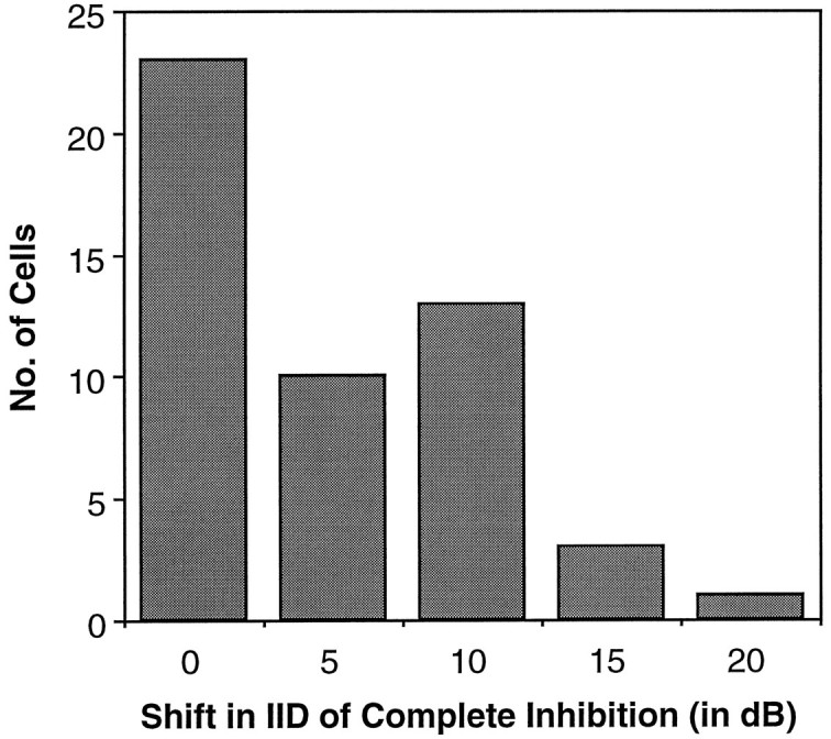
The distribution of shifts in the IID of complete inhibition from advancing the signal to the inhibitory ear. Thebar at 0 shift represents the 23 neurons with matched latencies, the IIDs of complete inhibition of which did not shift to less negative values. For the 27 neurons with mismatched latencies, the distribution of shifts in the IID of complete inhibition ranged from 5 to 20 dB. As in Figure 8, the shifts reported here represent the greatest degree of shift documented for each cell. All measures were made with the intensity at the excitatory ear fixed at 20 dB above threshold.

Neurons with mismatched latencies usually required relatively more intense signals at the inhibitory ear to reach complete inhibition than neurons with matched latencies

The average IID of complete inhibition from the population of neurons with matched latencies differed from that of the population of neurons with mismatched latencies. Figure 10 shows the distribution of IIDs of complete inhibition for both populations that were obtained when the signals were presented simultaneously to the two ears. Even though the range of the two distributions overlapped, the average IID of complete inhibition value for neurons with mismatched latencies was 8.9 dB less positive than the average IID of complete inhibition of neurons with matched latencies. This difference in IID of complete inhibition is statistically significant (t test: df = 48, t = 2.2; p < 0.05) and is consistent with the way in which a mismatch in latency should influence the IID of complete inhibition: a delayed inhibition requires a more intense inhibitory signal to reach complete inhibition. Moreover, the difference between the average of the two distributions (8.9 dB) corresponds to the average shift in the IID of complete inhibition (9.0 dB) generated by advancing the signal to the inhibitory ear. We interpret these results to mean that, in approximately half of the cells, latency differences or neural delays play a substantial role in determining the IID of complete inhibition and, therefore, IID selectivity. Finally, we wish to emphasize that the distinction between neurons with matched latencies and neurons with mismatched latencies is based solely on the relative latencies of excitation and inhibition. These cells seem to be identical in every other way.

Fig. 10.

Distribution of IIDs of complete inhibition for the 27 neurons with mismatched latencies and the 23 neurons with matched latencies. IIDs of complete inhibition were measured for both populations with simultaneous stimulation of the ears, i.e., with an ITD of 0 μsec.

DISCUSSION

The IID functions from the LSO of the free-tailed bat exhibited the same basic characteristics as seen in LSO cells in numerous other species (cat: Boudreau and Tsuchitani, 1968; Caird and Klinke, 1983;Tsuchitani, 1988; chinchilla: Finlayson and Caspary, 1991; gerbil:Sanes and Rubel, 1988; bat: Harnischfeger et al., 1985; Covey et al., 1991). However, to our knowledge, only one other study systematically investigated the range of IID selectivities exhibited by LSO neurons.Sanes and Rubel (1988) measured IID functions from gerbil LSO cells and found that IIDs of complete inhibition ranged from ∼+20 to −50 dB (their Fig. 15). This is remarkably similar to the range we found in the free-tailed bat. In both species, the range of IID selectivity corresponds to sound locations that would occur throughout most of the frontal sound field (Pollak, 1988; Sanes and Rubel, 1988).

Time–intensity trading

Each of the 50 cells from which we recorded showed time–intensity trading. There are two significant points associated with the time–intensity trading that we observed. First, the values of trading ratios found in the LSO (mean = 41 μsec/dB) are very similar to those reported previously for the inferior colliculus of the same species (mean = 47 μsec/dB; Pollak, 1988), indicating that the time–intensity trading seen in the colliculus may be, to a large extent, already established in the LSO. Second, because mammals experience IIDs in the range of tens of decibels for high frequency sounds (Erulkar, 1972), the time–intensity trading values we observed suggest that this phenomenon should significantly affect binaural processing in the LSO.

We wish to point out that we measured time–intensity ratios at relatively low-to-moderate overall intensities: the intensity to the excitatory ear was always set at 20 dB above threshold, and the intensity to the inhibitory ear was usually varied ±30 dB relative to that. Although we did not use extremely high intensities in our experiments, we would expect high intensities to compromise time–intensity ratios, because intensity-induced latency changes tend to saturate at high intensities (Kiang, 1965; Irvine and Gago, 1990;Joris and Yin, 1995).

ITD sensitivity

The ITD sensitivities that we observed were in the range of hundreds of microseconds, which is consistent with previous reports from other species (Finlayson and Caspary, 1991; Wu and Kelly, 1992;Joris and Yin, 1995). ITDs of this magnitude would not be experienced by the free-tailed bat under natural conditions. The small interaural distance of this species only creates ITDs of about 30–40 μsec (Pollak, 1988). Hence, in the free-tailed bat, as in other small mammals, ITDs per se probably do not significantly affect IID coding. However, as a sound source moves around the heads of larger animals, the changes in both ITDs and IIDs are sufficiently large that they both should affect their LSO targets. For a location favoring the excitatory ear, not only would the sound arrive at the excitatory ear first, but it would also be more intense at the excitatory ear. The effects of time–intensity trading would advance the excitation relative to the inhibition beyond that caused by its earlier arrival, allowing for free expression of the excitatory drive. For a location favoring the inhibitory ear, the sound would arrive earlier at the inhibitory ear and would be more intense at that ear. Both features should cause the inhibition to lead the excitation, but the higher intensity at the inhibitory ear should also increase the inhibitory duration, causing the stronger inhibition to overlap with the weaker excitation (as shown in Figs. 1, 6). Thus, for binaural coding in the LSO, the main effect of having a large head is that ITDs enhance the effects of IIDs.

Several mechanisms could influence response latency and strength

We used the term “latency” throughout this report to refer to the effects of the relative timing of excitation and inhibition at the postsynaptic cell rather than to their absolute latencies, which we did not evaluate. We used the term in that way because there are numerous factors, which our studies do not address, that influence response latency. One factor that could affect latency is the path length of excitatory and inhibitory fibers. This mechanism was first proposed byJeffress (1948) and is generally believed to be a major factor in the generation of ITD sensitivity in the medial superior olive of mammals and nucleus laminaris of birds. Another factor is axonal diameters and, thus, the conduction velocities of input fibers. Additional factors include density and arrangement of synapses, distribution and density of receptors, membrane resistance at the target cell, and the location of the spike-initiating zone. These mechanisms are not mutually exclusive, and it seems reasonable to suppose that they all contribute to the postsynaptic response latency of the cell.

Similar considerations apply to the way that we used the term “strength” of excitation and inhibition. For purposes of illustration in Figures 1 and 6, we showed equally strong effects from the two ears as equally large inhibitory and excitatory postsynaptic potentials. This may or may not be the case. The only requirement for equal strengths is that the conductance change caused by the inhibitory inputs be sufficiently large to prevent the excitation from reaching a threshold level. The indirect observations that we made allow us to conclude that the two effects had comparable strengths. Our data, however, do not address the issue of mechanisms for latencies or strengths, and it was for this reason that we used these terms operationally rather than mechanistically.

Latency mismatches were always in the same direction

It is of interest that longer latencies (neural delays) were always associated with the inhibitory inputs and never with the excitatory inputs: when the two inputs produced equally strong effects, the inhibitory latencies were always equal to or lagged behind the excitatory latencies. Given that the delays (latency differences) were on the order of hundreds of microseconds rather than milliseconds, there seems to be no compelling physiological reason why excitatory latencies could not have been longer than inhibitory latencies.

The diversity of IIDs of complete inhibition can be partially explained

The results presented previously suggest that there are at least two ways that latencies and strengths of excitation and inhibition are matched at the LSO, and the particular match can explain, in part, the diversity of IIDs of complete inhibition displayed by LSO cells. One way, exemplified by neurons with matched latencies, suggests that equal latencies are matched with equal strengths of excitation and inhibition. In most neurons with matched latencies, this matching is generated by IIDs of complete inhibition that are either at or near 0 dB or are positive and favor the excitatory ear. A second way, exemplified by neurons with mismatched latencies, suggests that equal strengths of excitation and inhibition are matched with noncoincident latencies. To bring the excitation and inhibition into coincidence, an extra intensity increment is required at the inhibitory ear. Thus, most neurons with mismatched latencies have negative IIDs of complete inhibition that favor the inhibitory ear. In summary, as IID of complete inhibition changes from favoring the excitatory to favoring the inhibitory ear, there is a progressive and corresponding shift from neurons with matched latencies to neurons with mismatched latencies.

Not all LSO neurons, however, have IIDs of complete inhibition that conform to the matching arrangement described above. As shown in Figure 10, some neurons with mismatched latencies had positive IIDs of complete inhibition that favor the excitatory ear, whereas in others it was at or near 0 dB. Conversely, some neurons with matched latencies had negative IIDs of complete inhibition that favor the inhibitory ear. The IIDs of complete inhibition of these cells, as well as other features, can be explained more comprehensively if we also assume that the inputs from each ear have different thresholds, in which the threshold difference corresponds to the intensity difference that produces equal strengths of excitation and inhibition. The value of adding this feature is not only that it offers a more complete explanation of the results, but it also makes specific predictions that can be tested experimentally.

For neurons with matched latencies, the excitation and inhibition always have the same latencies and equivalent strengths at the IID of complete inhibition, as discussed previously. If, in each matched latency neuron, the threshold difference is equal but opposite to the IID of complete inhibition, the threshold difference can compensate for the intensity disparity that would be generated by sound from a particular region of space. As an example, consider a matched latency neuron innervated by excitatory inputs that have higher thresholds than the inhibitory inputs (Fig. 11, panel 1). Although a sound in the ipsilateral sound field would be more intense at the excitatory (ipsilateral) ear than the inhibitory (contralateral) ear, the more intense sound would generate the same strength at the LSO cell as the less intense sound, because the thresholds of the excitatory fibers innervating that cell are higher than those of the fibers from the inhibitory ear. Thus, the model predicts that the cell should have a positive IID of complete inhibition. For the same reasons, if cells with matched latencies are innervated by excitatory inputs that have lower thresholds than the inhibitory inputs, these cells should have negative IIDs of complete inhibition (Fig. 11, panel 3). On the other hand, when the input thresholds are equal, the IID of complete inhibition of the cell should be 0 dB (Fig. 11, panel 2); thus, invoking threshold differences is essentially the same as a model proposed previously by Reed and Blum (1990; Blum and Reed, 1991).

Fig. 11.

Schematic models showing how the matching of thresholds and latencies from the two ears could create the variety of IIDs of complete inhibition (IID_ci) in neurons with matched latencies (panels 1–3) and in neurons with mismatched latencies (panels 4–7). Each LSO cell is innervated by several fibers (arrows) from the ipsilateral (excitatory) ear and several fibers from the contralateral (inhibitory) ear. The threshold of each fiber is indicated by its position relative to the target LSO cell: fibers with high thresholds are at thetop, and fibers with progressively lower thresholds are at the bottom. The latency of the input is indicated by the distance of each fiber from the target LSO cell. For neurons with mismatched latencies, the difference between the latencies of the excitatory and inhibitory inputs is indicated by a bar that separates the LSO cell from the inputs. Shown next to each LSO cell are three hypothetical records. Each record shows the relative strength and timing of excitation (top) and inhibition (bottom) that would be generated in the LSO cell by a sound at a particular location in the frontal sound field. The top records show the excitation and inhibition resulting from a sound in the ipsilateral field that would generate an IID that favors the excitatory ear, the middle records for a sound directly in front, and the bottom record for a sound in the contralateral sound field. The location that would result in equally strong excitation and inhibition is indicated on the rightof one of the three records.

For neurons with mismatched latencies, we propose that input thresholds are mismatched or matched as in neurons with matched latencies, but in addition there is a mismatch in latency. The latency mismatch is polarized in that the latency of the inhibition is always longer than the latency of the excitation. In terms of its influence on the IID of complete inhibition, the latency increment of the inhibition has the same effect as raising the threshold of the inhibitory input: to achieve coincidence, the cell requires a more intense inhibitory signal than it would if there were no delay, which creates a less positive (or more negative) IID of complete inhibition. In Figure 11, for example, the threshold difference for the matched latency neuron in panel1 would create a positive IID of complete inhibition, generated by a sound in the far ipsilateral sound field. The same threshold difference with a latency mismatch would create a less positive IID of complete inhibition, generated by a sound closer to the midline (Fig. 11, panel 4). A similar effect attributable to a latency mismatch can also be seen for neurons with equal thresholds in panels 5 and 7 of Figure 11. This hypothesis for neurons with mismatched latencies is consistent with the latency hypothesis model.

In summary, the results suggest that the matching of strengths and latencies from the two ears, in the two ways exemplified by neurons with matched latencies and those with mismatched latencies, are features that contribute to the diversity of IID selectivity in the LSO. However, these features by themselves do not account for the properties of all LSO neurons. We propose that the range of IID selectivities in the LSO population can be explained more fully by a model that matches differences in strengths and latencies with threshold differences, and the predictions made by the model can be tested in future experiments.

REFERENCES

- 1.Blum JJ, Reed MC. Further studies of a model for azimuthal encoding: lateral superior olive neuron–response curves and developmental processes. J Acoust Soc Am. 1991;90:1968–1978. doi: 10.1121/1.401676. [DOI] [PubMed] [Google Scholar]
- 2.Boudreau JC, Tsuchitani C. Binaural interaction in the cat superior olive S-segment. J Neurophysiol. 1968;31:442–454. doi: 10.1152/jn.1968.31.3.442. [DOI] [PubMed] [Google Scholar]
- 3.Caird D, Klinke R. Processing of binaural stimuli by cat superior olivary complex neurons. Exp Brain Res. 1983;52:385–399. doi: 10.1007/BF00238032. [DOI] [PubMed] [Google Scholar]
- 4.Covey E, Vater M, Casseday JH. Binaural properties of single units in the superior olivary complex of the mustached bat. J Neurophysiol. 1991;66:1080–1094. doi: 10.1152/jn.1991.66.3.1080. [DOI] [PubMed] [Google Scholar]
- 5.Erulkar SD. Comparative aspects of spatial localization of sounds. Physiol Rev. 1972;52:237–360. doi: 10.1152/physrev.1972.52.1.237. [DOI] [PubMed] [Google Scholar]
- 6.Finlayson PG, Caspary DM. Low-frequency neurons in the lateral superior olive exhibit phase-sensitive binaural inhibition. J Neurophysiol. 1991;65:598–605. doi: 10.1152/jn.1991.65.3.598. [DOI] [PubMed] [Google Scholar]
- 7.Harnischfeger G, Neuweiler G, Schlegel P. Interaural time and intensity coding in superior olivary complex and inferior colliculus of the echolocating bat Molossus ater. J Neurophysiol. 1985;53:89–109. doi: 10.1152/jn.1985.53.1.89. [DOI] [PubMed] [Google Scholar]
- 8.Irvine DRF. Auditory brainstem processing. In: Popper AN, Fay RR, editors. The mammalian auditory pathway: neurophysiology. Springer; New York: 1992. pp. 153–231. [Google Scholar]
- 9.Irvine DRF, Gago G. Binaural interaction in high-frequency neurons in inferior colliculus of the cat: effects of variation in sound pressure level on sensitivity to interaural intensity differences. J Neurophysiol. 1990;63:570–591. doi: 10.1152/jn.1990.63.3.570. [DOI] [PubMed] [Google Scholar]
- 10.Irvine DRF, Park VN, Mattingley JB. Responses of neurons in the inferior colliculus of the rat to interaural time and intensity differences in transient stimuli: implications for the latency hypothesis. Hear Res. 1995;85:127–141. doi: 10.1016/0378-5955(95)00040-b. [DOI] [PubMed] [Google Scholar]
- 11.Jeffress LA. A place theory of sound localization. J Comp Physiol Psychol. 1948;41:35–39. doi: 10.1037/h0061495. [DOI] [PubMed] [Google Scholar]
- 12.Joris PX, Yin TCT. Envelope coding in the lateral superior olive. I. Sensitivity to interaural time differences. J Neurophysiol. 1995;73:1043–1062. doi: 10.1152/jn.1995.73.3.1043. [DOI] [PubMed] [Google Scholar]
- 13.Kiang NY-S. Stimulus coding in the auditory nerve and cochlear nucleus. Acta Otolaryngol. 1965;59:186–200. [Google Scholar]
- 14.Pollak GD. Time is traded for intensity in the bat’s auditory system. Hear Res. 1988;36:107–124. doi: 10.1016/0378-5955(88)90054-8. [DOI] [PubMed] [Google Scholar]
- 15.Reed MC, Blum JJ. A model for the computation and encoding of azimuthal information by the lateral superior olive. J Acoust Soc Am. 1990;88:1442–1453. doi: 10.1121/1.399721. [DOI] [PubMed] [Google Scholar]
- 16.Sanes DH. An in vitro analysis of sound localization mechanisms in the gerbil lateral superior olive. J Neurosci. 1990;10:3494–3506. doi: 10.1523/JNEUROSCI.10-11-03494.1990. [DOI] [PMC free article] [PubMed] [Google Scholar]
- 17.Sanes DH, Rubel EW. The ontogeny of inhibition and excitation in the gerbil lateral superior olive. J Neurosci. 1988;8:682–700. doi: 10.1523/JNEUROSCI.08-02-00682.1988. [DOI] [PMC free article] [PubMed] [Google Scholar]
- 18.Schlegel P. Calibrated earphones for the echolocating bat, Rhinolophus ferrunequinum. J Comp Physiol [A] 1977;118:353–356. [Google Scholar]
- 19.Schuller G, Radtke-Schuller S, Betz M. A stereotactic method for small animals using experimental determined reference profiles. J Neurosci Methods. 1986;18:339–350. doi: 10.1016/0165-0270(86)90022-1. [DOI] [PubMed] [Google Scholar]
- 20.Tsuchitani C. The inhibition of cat lateral superior olive unit excitatory responses to binaural tone-burst. I. The transient chopper response. J Neurophysiol. 1988;59:164–183. doi: 10.1152/jn.1988.59.1.164. [DOI] [PubMed] [Google Scholar]
- 21.Wu SH, Kelly JB. Binaural interaction in the lateral superior olive: time difference sensitivity in the mouse brain slice. J Neurophysiol. 1992;68:1151–1159. doi: 10.1152/jn.1992.68.4.1151. [DOI] [PubMed] [Google Scholar]
- 22.Yin TCT, Hirsch JA, Chan JCK. Response of neurons in the cat’s superior colliculus to acoustic stimuli. II. A model of interaural intensity sensitivity. J Neurophysiol. 1985;53:746–758. doi: 10.1152/jn.1985.53.3.746. [DOI] [PubMed] [Google Scholar]