The Analysis of Complex Motion Patterns by Form/Cue Invariant MSTd Neurons

Abstract

Several groups have proposed that area MSTd of the macaque monkey has a role in processing optical flow information used in the analysis of self motion, based on its neurons’ selectivity for large-field motion patterns such as expansion, contraction, and rotation. It has also been suggested that this cortical region may be important in analyzing the complex motions of objects. More generally, MSTd could be involved in the generic function of complex motion pattern representation, with its cells responsible for integrating local motion signals sent forward from area MT into a more unified representation. If MSTd is extracting generic motion pattern signals, it would be important that the preferred tuning of MSTd neurons not depend on the particular features and cues that allow these motions to be represented. To test this idea, we examined the diversity of stimulus features and cues over which MSTd cells can extract information about motion patterns such as expansion, contraction, rotation, and spirals. The different classes of stimuli included: coherently moving random dot patterns, solid squares, outlines of squares, a square aperture moving in front of an underlying stationary pattern of random dots, a square composed entirely of flicker, and a square of nonFourier motion. When a unit was tuned with respect to motion patterns across these stimulus classes, the motion pattern producing the most vigorous response in a neuron was nearly the same for each class. Although preferred tuning was invariant, the magnitude and width of the tuning curves often varied between classes. Thus, MSTd is form/cue invariant for complex motions, making it an appropriate candidate for analysis of object motion as well as motion introduced by observer translation.

Two pathways for visual information processing in extrastriate cortex have been identified (Ungerleider and Mishkin, 1982; Van Essen and Maunsell, 1983; DeYoe and Van Essen, 1988). One stream, the “what” pathway, sends information ventrally into the temporal lobe and appears to be involved in processing the spatial pattern of the visual scene. The other stream, projecting dorsally into posterior parietal cortex, has been described as the “where” pathway and is involved in localizing objects in space and the related task of processing image motion. The best-studied area with regard to the latter task is area MT, located on the posterior bank and floor of the superior temporal sulcus (STS), containing cells shown to respond to simple linear (translational) motion (Maunsell and Van Essen, 1983a,b; Albright, 1984). MT sends a heavy projection forward to area MST (medial superior temporal region), an adjacent cortical region located on the floor and anterior bank of the STS. Area MST, which is also believed to play an important role in the motion processing hierarchy, has been functionally segmented into at least two distinct regions, a ventral lateral one (MSTl) and a dorsal one (MSTd) (Desimone and Ungerleider, 1986; Saito et al., 1986; Ungerleider and Desimone, 1986a,b; Komatsu and Wurtz, 1988). The cells in MSTl have been shown to have relatively small receptive fields, rather similar in size to those found in area MT at the same eccentricity and also similar in terms of their preference for translational motion. Cells in MSTd, on the other hand, have comparatively large receptive fields that generally include the fovea and often extend across both ipsi- and contralateral hemifields. These cells are selectively tuned not only for large-field translational motion, but also for motion patterns such as expansion, contraction, and rotation (Sakata et al., 1985; Saito et al., 1986;Tanaka et al., 1986, 1989; Tanaka and Saito, 1989). Our lab’s previous investigation in MSTd also showed that some units in this region have complex response characteristics, in many cases demonstrating a preference for spiraling motion patterns over expansion, contraction, and rotation (Graziano et al., 1994).

Because these complex motion patterns are built up from local regions of approximately straight motion, they can effectively drive many directionally selective units in MT. What distinguishes a large proportion of MSTd cells, besides the increased size of their receptive fields, is that their specificity for motion pattern is not sensitive to stimulus placement within a neuron’s receptive field (Duffy and Wurtz, 1991a,b; Graziano et al., 1994), a property referred to as positional invariance. The invariance is with respect to preferred tuning and is less pronounced for response amplitude (Duffy and Wurtz, 1995) and tuning width. Tuning invariance with respect to motion pattern is not found within MT, where even minor positional shifts in the placement of the these stimuli can dramatically alter (even reverse) a unit’s preferred tuning (Lagae et al., 1994).

The types of complex motion stimuli to which MSTd cells respond have been associated with the full field patterns projected onto the retina during observer locomotion, as first recognized by Gibson (1950). Many computational and psychophysical studies have shown that by analyzing these flow-field motion patterns and detecting such features as the focus of expansion, the parameters of observer rotation and translation can be recovered (Prazdny, 1980; Andersen, 1986; Warren and Hannon, 1990). This suggests a role for MSTd in processing ego-motion and determining direction of heading (DOH). At face value, the well documented positional invariance of MSTd units is puzzling—if the nervous system uses optical flow to guide navigation, we might expect neurons performing DOH analysis to be sensitive to the retinal location of these patterns. However, positional invariance with respect to stimulus specificity does not preclude changes in the response amplitude with stimulus placement (Duffy and Wurtz, 1995). A coarse-coding scheme could take advantage of a spatial response gradient to encode the location of the focus of expansion by pooling information over a large number of units.

Although there is good evidence that MSTd is important in the analysis of optical flow, the positional invariance of these units with respect to preferred tuning suggests other possible roles. An additional function for MSTd makes an analogy between MSTd and area IT (inferotemporal cortex) in the temporal lobe (Graziano et al., 1994), which also demonstrates positional invariance. Cells in IT have been found that are selective for such complex spatial patterns as toilet brushes and faces (Gross et al., 1972; Desimone et al., 1984). This selectivity is maintained regardless of stimulus placement within the units’ large receptive fields (Schwartz et al., 1983; Desimone et al., 1984). The positional invariance in cell tuning for both IT and MSTd suggests a functional connection between the two areas. Where IT is thought to analyze spatial pattern information in the image, MSTd could analyze motion pattern information. It should be emphasized that the possible “pattern” motion and “ego-motion” roles for MSTd are not mutually exclusive. In fact, ego-motion analysis can be considered a subtype of pattern motion processing. MSTd might also be important as an early stage in analysis of biological motion, such as that presented in Johansson dot displays (Hoffman and Flinchbaugh, 1982; Poizner and Bellugi, 1981; Mather et al., 1992; Dittrich, 1993; Mather and West, 1993).

Many experiments studying area MSTd have used random dot (RD) stimuli with different types of global motion (expansion, contraction, translation motion, etc.) to probe the response properties of these cells. In the current investigation, we have included stimuli, the motion pattern of which is established by features other than random dots, such as edges, and then compare these responses and tuning curves across classes. We also explore the effect of using cues other than luminance by creating motion patterns using “second-order” or nonFourier motion. These experiments will help to establish how general the features and cues are that MSTd uses to extract motion pattern. This work is partially motivated by studies of “form/feature/cue invariance” recently demonstrated in MT, V1, and IT (Albright and Chaudhuri, 1989; Albright, 1992; Sary et al., 1993).

MATERIALS AND METHODS

Animal preparation. Three hemispheres from two Rhesus monkeys were used for these experiments. Because the results were similar in the two monkeys, the data were pooled for the purpose of analysis. Units located in MSTd were tentatively identified based on their location in the chamber and depth relative to the dura. In each of the three chambers recorded from, we mapped out both MSTd and MT based on the tuning characteristics of cells in these regions. Particularly helpful in distinguishing MSTd from MT was the former cells’ large receptive fields and positional invariance. Based on these initial criteria, 190 cells were considered for analysis, 71 from monkey 89-1 and 119 from monkey 90-2. The details of the recording procedure have been described previously (Graziano et al., 1994). Briefly, a scleral search coil and an acrylic skull cap were implanted 5 d before beginning training on a fixation task. Training and subsequent behavior were reinforced by depriving the monkeys of fluid before each session and then giving drops of apple juice upon correct task completion. After mastery of the behavior, a second surgery was performed to introduce a craniotomy that provided chronic access to the brain for recording purposes. Because we were confident of our identification of area MSTd based on approximate location and response properties, we chose not to kill the monkeys for purposes of anatomy. These monkeys went on to become subjects in subsequent investigations.

Fixation task and data collection. The animal was placed 57 cm away from a wide-field tangent screen projection monitor, which readily allowed stimuli as large as 40° in diameter to be presented to the monkey. Trials were initiated by the appearance of a green (0.1°) fixation point directly ahead of the animal. The monkey was required to fixate the target and pull a lever within 600 msec of target onset. After a 3 sec period, which included the presentation of two stimuli and an intervening gap, the fixation point dimmed and the monkey was required to release the lever to receive a reward. Throughout the trial, eye position was monitored. If eye speeds exceeded 15°/sec (as in a saccade), the trial was terminated without a reward. Data collection was controlled by a PDP-11 computer, and stimulus presentation was controlled by a PC-compatible 386 computer.

Stimuli. The different visual stimuli used can be divided into different types and classes. A stimulus’s class refers to attributes of the stimulus other than motion pattern; i.e., whether its features are composed of random dots, lines (empty square), edges (solid square), aperture borders, or flicker. A stimulus’s type refers to the motion pattern these features undergo relative to one another, namely, whether they expand, rotate, contract, or spiral.

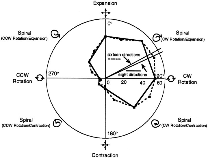
Stimulus type is based on the concept of a spiral space (Fig.1), originally formulated in Graziano et al. (1994). In this space, expansion and contraction are on opposite sides of the same axis, and the two directions of rotation are on opposite sides of the orthogonal axis. A stimulus, the image features of which have their motion vectors pointed 180° away from the center of the display (expansion), is represented straight up in this space (0°); contraction is represented straight downward (180°). Moving from expansion to contraction is equivalent to rotating the velocity vectors of the features by 180°. If, instead, these vectors are rotated 90°, global rotation in either direction is obtained. For example, rotating the velocity vectors of an expansion stimulus 90° clockwise results in a clockwise rotation stimulus pattern. Intermediate rotations, such as the 45° rotations used in these experiments, result in spirals. Spirals contain elements of either expansion or contraction combined with either clockwise or counterclockwise rotation, giving four basic types of spiral pattern. Using this representation, a continuous space is formed, with expansion, rotation, and contraction being discrete cardinal directions within this “spiral” space (Fig. 1).

Fig. 1.

Spiral space explained. In this representation, expansion/contraction are on opposite sides of the vertical axis, and the two directions of rotation are on opposite sides of the horizontal axis. Intermediate orientations between these cardinal axes represent spiral patterns. Expansion (top) is assigned an angular value of 0° by convention, with the angles increasing as one moves clockwise. Distance from the origin is a measure of firing rate; angle reflects the type of motion pattern. Data from the two curves displayed on this polar plot were obtained from a single cell using the RD stimulus class. With one curve, the space was sampled every 22.5° (16 points), and with the other curve every 45° (8 points). Each point plotted represents the average firing rate for that stimulus type (motion pattern) pooled from repeated, randomly interleaved trials. Note the similarity of the two curves obtained at the two sampling frequencies. The lines emanating from the origin represent the preferred tuning directions recovered from this data after regression to Gaussians. This particular unit was tuned to a spiral containing elements of both expansion and clockwise rotation. The similarity of tuning curves for the two sampling densities enabled us to use the lower sampling frequency so that more data could be collected per recording session.

A stimulus “movie” is composed of 60 consecutive image frames lasting a total of 1 sec. Six classes of stimuli were used, four of which are represented in Figure 2. The RD class (for details, see Graziano et al., 1994) consists of 150 dots with limited lifetimes (333 msec, or 20 frames) and constant velocity. At the end of its lifetime, each dot is assigned a new random location within the 20° diameter stimulus circle and given a trajectory and speed appropriate for its new location. The dots are relocated asynchronously to avoid a coherent flickering of the stimulus every 333 msec. If the dot moved outside the bounds of the display window, it was immediately assigned a new, random location within the display circle and given a new trajectory. For all stimulus types (patterns), the speed of each dot was a linear function of its distance from the center of the display, in this case given by the formula S = 0.2 × r, where S is in (distance units)/sec andr is in distance units. The direction of motion for each dot is determined by the type of global motion desired (e.g., expansion requires each dot to be moving directly away from the center of the stimulus).

Fig. 2.

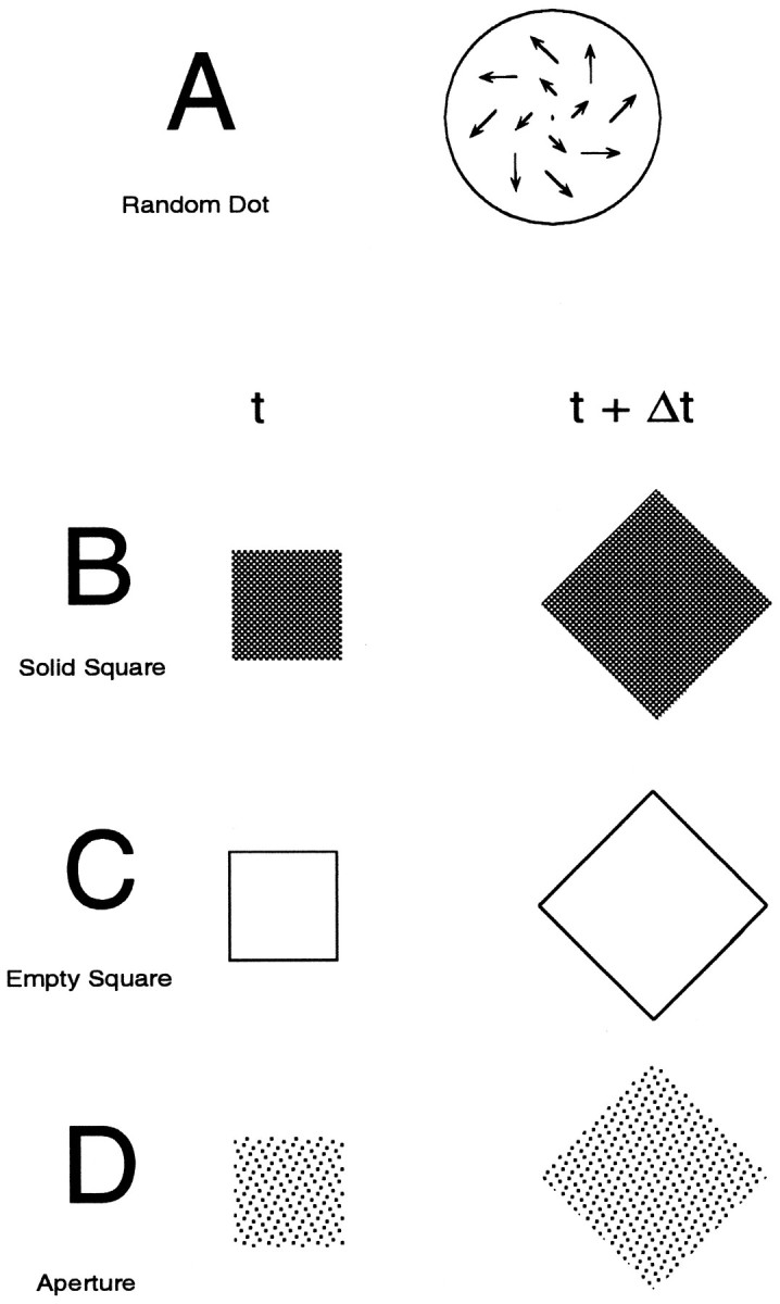
Four of the six stimulus classes. Ashows the velocity vector field for a spiral midway between expansion and counterclockwise rotation (corresponding to an angular location of 315° in spiral space). Note that the lengths of these vectors increase with distance from the center of the stimulus. B–Dshow representative frames from different stimulus classes at two points in time. Because the squares represented are both rotating and expanding with time, their motion pattern is also that of a spiral. In the AP class, the texture elements making up the interior of the square do not move with the edges of the stimulus. The spacing and placement of these texture elements remain unchanged. Although the patterns are all represented as black against a white background, on the screen the polarity was reversed. The luminance contrasts of the AP and SS classes were actually more similar than they appear in this figure. Two additional classes, FL and NF, also were used in this study, but the nature of these stimuli prevented a convenient static representation.

RD stimuli are incompatible with the motion of a single object. For example, although the dots in the expansion stimulus move outward with motion consistent with the approach of an object, the circular boundary of this stimulus is stationary. As this luminance boundary is readily visible because of the relatively high density of dots within the stimulus, an observer does not get the impression of a single approaching circular object. Instead, the dots appear as independent features.

A second distinguishing feature of the RD stimuli is that they do not evolve during their 1 sec presentations. The instantaneous velocity fields don’t change during the stimulus sequence. Psychophysical evidence exists suggesting that such pure “velocity fields,” despite giving rise to some ambiguities, are sufficient in many cases to allow observers to recover DOH (Warren and Hannon, 1988). For these reasons, we think of this stimulus class as being “flow-like” because it captures aspects of global motion pattern sufficient for ego-motion while leaving out stimulus attributes, which may be important in the perception of moving objects in the environment.

Two other stimulus classes, solid square (SS) and empty square (ES), were created by having the corners of squares obey motion rules similar to those established for the RD stimuli (Fig. 2). However, whereas the dots of the RD class have limited lifetimes and straight paths, the borders of the squares are visible for the entire movie and have acceleration and curvature consistent with their trajectories being updated every frame. These stimuli simulate the motion of a single, rigid object. Only the edges of the SS and ES stimuli contain information about the motion of the stimulus, which is exactly opposite the case for the RD stimulus class. The inclusion of both the ES and SS classes was motivated by looming detectors in other species, which respond well to SS type stimuli but poorly to ES stimuli (Simmons and Rind, 1992).

The aperture (AP) stimuli were created by moving a virtual window, identical in spatial extent and motion pattern to the squares in the ES and SS classes, over a stationary background of random dots with unlimited lifetime (Fig. 2). The background is hidden except where the square aperture window exposes the RD background underneath. The spacing between the dots remains constant, and the dots themselves have no motion, other than to be exposed or occluded with time, depending on the motion pattern specified for the aperture.

The flicker (FL) stimuli were identical to the SS stimuli described above, except that instead of the interior of the square being a homogeneous gray, it consisted of random pixels turning on and off every frame, creating a shimmering interior to the square. Dot density was adjusted so that the luminance contrast of the square against the background was the same as the SS case. For the ES, SS, FL, and AP classes, the minimum size of the square is 5° of visual angle as viewed by the monkey. This occurs for the first frame of an expansion pattern and the last frame of a contraction pattern. Maximum edge-length is 20°. The presence of flickering dots has been shown to inhibit the directional response of area MT (Snowden et al., 1991) cells, and we were interested in examining a similar effect in area MSTd.

The nonFourier (NF) stimulus was produced by creating a 20° square field of small squares that each have a 50% probability of being on or off, with each square covering 0.1° of visual angle. Pixel polarity does not change from frame to frame unless the imaginary border of a square obeying motion rules identical to those established for the squares described above passes over the pixel in question. Where this occurs, the polarity of the pixel reverses every frame that the virtual square border is over the pixel. Using this method, the motion of the border was readily visible to human observers at the eccentricities used in these experiments. Unlike the other classes, motion pattern is not defined by luminance cues, but by flicker in the stimulus. A study by Albright (1992) showed that units in MT can respond to translational motion defined by this cue reasonably well, and we were interested to see whether this was also the case in MSTd.

In the discussion that follows, an experiment refers to data recorded using a single stimulus class (RD, SS, ES, FL, AP, or NF) for each of the eight motion types (expansion, contraction, two types of rotation, and four types of spirals) in multiple repeats (approximately eight) of each stimulus. Figure 1 shows two superimposed tuning curves obtained by sampling 8 and 16 directions in spiral space. As demonstrated in this figure, during preliminary experiments we determined that using 8 evenly spaced stimulus directions gave similar response profiles as 16 directions. We chose to sample at the lower density to save recording time. Therefore, a single experiment has approximately 64 trials (8 repeats of the 8 stimulus types). Sometimes less data were collected when we were unable to hold the cell or when the monkey would not cooperate with the behavior. We performed up to six different experiments on each cell, one for each stimulus class. The stimuli were all generated off-line before the experiments and displayed during the trials at a refresh rate of 60 Hz.

ANALYSIS

Regression and hypothesis testing was used extensively to analyze the data. Some of these techniques are strictly valid only when linear models are considered. Because much of the time the curve fits are nonlinear in their parameters (e.g., Gaussians), the probabilities calculated are approximations. However, for large N, the various indexes used approximate actual probabilities (Snedecor and Cochran, 1989).

One stage of the analysis involved plotting average firing rate against stimulus direction in spiral space for each experiment and then fitting the data to a Gaussian function. For many experiments, the response profile was essentially flat, making the Gaussian function inappropriate for modeling the data. A screening process was used to eliminate the experiments that produced flat response profiles. This involved regressing the data in each experiment to the horizontal line (response = constant) and then testing the hypothesis that the observed data were generated by a cell with a response profile adequately described by this equation. This “flat model” is the appropriate model for experiments in which stimulus type has no consistent effect on cell responsiveness.

To test the flat model’s goodness of fit for the data, an ANOVA was performed to determine the two components of the residual variance. The within-stimulus type variance is associated with the intrinsic variability of the data collected and is obtained according to the formula:

$$s_e^2=\frac{1}{N-n}\sum \sum (y_{\text{ij}}-\overline{y_{i·}}{)}^2,$$ Equation 1

where s²_e is an unbiased estimate of the within trial variance, N is the total number of trials from the experiment, n is the number of stimulus types, y_ij is the firing rate of thejth repeat of the ith stimulus type, and y_i· is the mean firing rate for the ith stimulus type (recall that stimulus type refers to the motion pattern of the stimulus in spiral space.) This variance could be calculated because data were collected for multiple repeats (6–10) of each stimulus. The remainder of the variance is the “lack of fit” variance. It is equal to the total variance less the within-trial variance. This value is large for the flat model on cells responding preferentially to different types of motion pattern. It represents the model’s lack of fit with respect to the data that cannot be explained after the variance associated with randomness in cell response is subtracted.

The quotient obtained by dividing this lack-of-fit variance by the within-trial variance is distributed according to an Fdistribution with 7 and N − 8 df, where Nis the total number of trials for the experiment (usually Nis ∼80). By determining where this quotient lies on the appropriateF curve, this value can be converted into a probability that is an unbiased measure of how well the data fits the model. The larger this value, the better the fit. This probability measure will be referred to as the flat index (FI) and has a minimum value of 0 and a maximum value of 1. The FI represents the probability that the observed lack of fit from the flat model can be explained by chance. Note that the variance quotient is large (and the FI small) when the lack of fit is large and the within-trial variance is small.

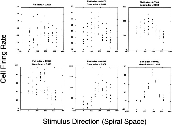
Figure 3 shows data from eight representative experiments reflecting a range of FIs. As described below, this same technique is used to test the goodness of fit for the Gaussian models recovered from these same data sets. We chose to be very conservative and only excluded from further analysis those experiments in which the observed lack of fit would have occurred at least 95% of the time by chance (i.e., an FI of >0.95), assuming the flat model was valid.

Fig. 3.

Raw data demonstrating various FIs and GIs. Moving across and then down, the data increasingly take on a more Gaussian-shaped profile. The variability of the data also decreases. No GI appears for the first data set because the FI exceeded 0.95. The second frame shows data from an experiment near our threshold criteria for exclusion based on the FI. Multiple data points within a particular graph for the same tuning direction represent repeated trials. Before curves could be fit, the data were shifted so that the preferred stimulus was centered at ∼180°. This facilitated regression in an analysis package that did not provide for circular statistics. Therefore, it was not the case that the units in the six experiments all had their preferred tuning direction near 180°. After regression, the mean parameter was shifted back in the opposite direction by an equivalent amount.

The experiments passing the above test were then regressed to a general Gaussian function with four parameters—floor, amplitude, mean, and width, according to the general formula:

$$y=a+b\times {exp}^{-(x-c{)}^2/d^2},$$ Equation 2

where the dependent variable y is firing rate and the independent variable x is stimulus direction in spiral space. The four adjustable parameters are as follows: a is the floor of the Gaussian function, b is the amplitude,c is the mean, and d is the variance (width). This choice was made for two reasons. As can be seen in the final frame of Figure 3, when a unit in MSTd gives a strongly selective response, the profile approximates a Gaussian quite well. Secondly, the four Gaussian parameters effectively characterize relevant aspects of a neuron’s response, such as preferred tuning.

The statistics package Systat was used to obtain these fits, along with confidence intervals for each parameter. Mean square error was used for the loss function. Hypothesis testing was performed as was done for the flat model above, substituting the best fit Gaussian model in place of the flat model. Lack of fit was calculated by subtracting the within-trial variance from the total variance, then dividing by the within-trial variance. Where this quotient fell along the appropriateF distribution recovered the probability that the observed lack of fit occurred by chance.

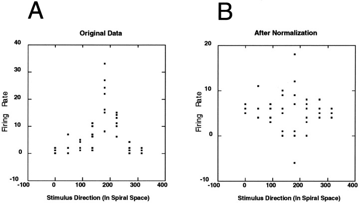
An index for differential response strength was needed for the analysis. Directional indexes that take into account only average preferred and anti-preferred responses are lacking in that they ignore aspects of the response profile provided by intermediate stimulus directions. Furthermore, it is desirable for an index of response strength to reflect the within-type response variability of the data. The smaller this variability, the greater the representational power of a unit for a particular stimulus attribute. What was desired, in essence, was an index of “Gaussianness” that would reflect both response amplitude and variability. To do this, the observed data were statistically compared against an appropriate “flat” set of data. To obtain the flat data, the average firing rate across all trials was determined for each individual experiment, and then the data were shifted for each trial so that the average firing rate was the same for all eight stimulus types (Fig. 4). In this way, the data were “flattened.” The within-trial variance remains unchanged after this transformation, allowing meaningful and powerful comparisons with the original data set.

Fig. 4.

“Flattening” of the data. A, The raw data from one experiment (i.e., one stimulus class, multiple motion types). This graph is identical in form to those described in Figure 3. The horizontal axis represents the motion pattern of the inducing stimulus. The vertical axis reports the magnitude of the response (in spikes/sec) to the stimulus. B, This plot shows the consequence of “flattening” the data, as outlined in the text. The within-trial variance, as well as the mean firing rate with respect to the entire data set, remains constant, but the average firing rate is now the same across all stimulus directions. By statistically comparing the top and bottom data sets, we achieved a measure of differential response strength.

Based on the Gaussian model recovered from the original data, the lack-of-fit statistic was calculated twice for each experiment, once on the original data and once on the flattened data. In all cases, the lack of fit of the Gaussian model to the original data was not significant. In most cases, the lack of fit for the flattened data was larger, particularly when the area under the model Gaussian curve was large. For each experiment, the log ratio of the two probabilities was calculated. This Gaussian index (GI) agrees well with subjective assessments of the Gaussianness of the data, as seen in Figure 3, and is an excellent measure of differential response strength. This figure shows experiments representing a range of GIs and FIs. Note that a GI is not calculated for the first experiment; in this case, the FI was above the threshold exclusion criteria of 0.95.

Circular, nonparametric statistics

Nonparametric tests from circular statistics were used to supplement the previous analysis (for a discussion of these methods, see Drew and Doucet, 1991; Fisher, 1993). Circular statistics address problems specific to the analysis of data, where the measured quantity is a function of a variable confined to a periodic input range. Nonparametric tests have the advantage of not requiring the shape of the tuning curves to conform to a particular model. Therefore, analysis of the data with these methods does not require previous screening of the experiments. The preferred tuning of a cell was calculated as the trigonometric mean of the data from the following equations:

$$\hspace{0.5em}C=\sum _{i=1}^n F_{i}cos{\phi }_i,S=\sum _{i=1}^n F_{i}sin{\phi }_i,\overline{\phi }=\text{arctan}(S/C),$$ Equation 3

where $\overline{\phi }$ is the preferred tuning of the cell (adjusted to the proper quadrant based on the signs of S andC), n is the number of directions in spiral space sampled (in this case 8), φ_i is direction in spiral space of the stimulus, andF_i is the average firing rate of the neuron in response to motion type i. According to the Rayleigh test, the null hypothesis (that the data are distributed uniformly; i.e., each motion type drives the cell by an equal amount) is rejected if p < 0.05 according to:

$$\overline{R}=\frac{\sqrt{S^2+C^2}}{\sum _{i=1}^n \text{Fi}},P=exp(-N\overline{R^2}),$$ Equation 4

where N is the total number of trials run during the experiment. $\overline{R}$ (the sample circular variance) is a measure of a cell’s selectivity (width of tuning curve) and is restricted to values between 0 and 1 with higher numbers reflecting wider tuning. To test whether the preferred tuning of two experiments is equal, we calculate:

$$\overline{C_2}=\left(1/\sum _{i=1}^n F_i\right) \sum _{i=1}^n F_{i}cos2{\phi }_i,$$

$$\overline{S_2}=\left(1/\sum _{i=1}^n F_i\right) \sum _{i=1}^n F_{i}sin2{\phi }_i,$$

$$\hspace{0.5em}{\widehat{\eta }}^2=\overline{C_2^2}+\overline{R_2^2},\delta =(1-{\widehat{\eta }}^2)/(2\overline{R^2}),{\varsigma }^2=\delta /N,$$

$$C_M=cos{u}_k/{\varsigma }_k^2+cos{u}_l/{\varsigma }_l^2,S_M=sin{u}_k/{\varsigma }_k^2+sin{u}_l/{\varsigma }_l^2,$$

$$R_M=\sqrt{C_M^2+S_M^2},Y=2(1/{\varsigma }_l^2+1/{\varsigma }_k^2-R_M),$$ Equation 5

where the hypothesis of a common preferred tuning underlying experiments l and k with trigonometric meansu_l andu_k was rejected if Y > 3.84. This limit corresponds to the upper 95% point of the chi-square distribution (with 1 df).

RESULTS

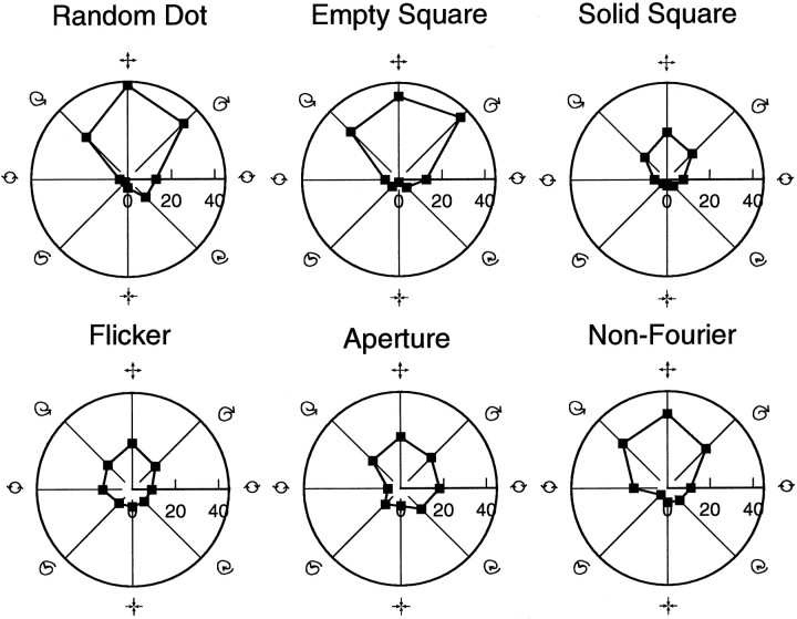
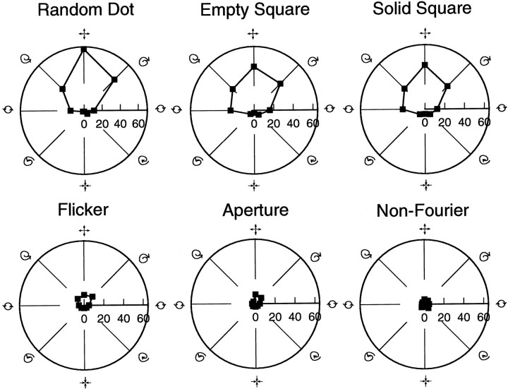
The basic findings of this study are reported in Figure5. This diagram shows polar plot tuning curves from a single cell in which each of the six stimulus classes gave tuned responses. This unit is tuned for expansion regardless of the features and cues used to define the motion patterns. For the AP class, although the response to expansion was strong, selectivity for stimulus pattern was somewhat less than for the other classes; a significant response to clockwise-rotating apertures was also recorded. Note that response amplitude and width does not possess the same degree of invariance as preferred tuning.

Fig. 5.

Comparison of tuning curves from a single unit for the six stimulus classes. This comes from one of the few cells (B10800) in which the FI and GI criteria were met for all six experimental classes. The location of each data point in these polar plots reflects both the magnitude of the response and the stimulus type used to elicit the response. Distance away from the origin indicates response strength in spikes per second, and the angle is a function of the stimulus motion pattern inducing this response. This particular unit is tuned for expansion. Note the similarity in the six curves in terms of both orientation and shape, although there is some variation with the AP class. Compared with Figure 4, tuning specificity is less pronounced; this unit also responds fairly strongly to clockwise rotational motion.

This unit is somewhat unusual in responding strongly to all six stimulus classes. An example of a cell responding to a subset of the classes is reported in Figure 6, which shows tuning curves for another unit tuned to expansion. Responses to FL, AP, and NF stimuli were 10 times weaker than to RD, ES, and SS with respect to average firing rate. However, except for the NF class, in which little selectivity is observed, a preference for expansion is maintained. This invariance with respect to stimulus class was generally observed for all the MSTd neurons recorded from.

Fig. 6.

Form/cue invariance of a single neuron. As with the cell in Figure 5, this unit is also tuned for expansion. Responses to the FL, AP, and NF classes are 10 times weaker than those to the RD, SS, and ES classes. The responses to the NF stimuli were not well tuned; little selectivity in response is demonstrated. This is likely a function of the poor signal-to-noise ratio associated with the low firing rates obtained from these stimuli.

Response strength and experiment screening

Although data from individual neurons strongly supports form/cue invariance in MSTd, it was important to quantify and formalize these findings over a population of MSTd units. We also wanted to compare response strength across stimulus class and relate this index to the degree of form/cue invariance. Because this analysis depends on quantifying differential response strength, this measure will be considered first.

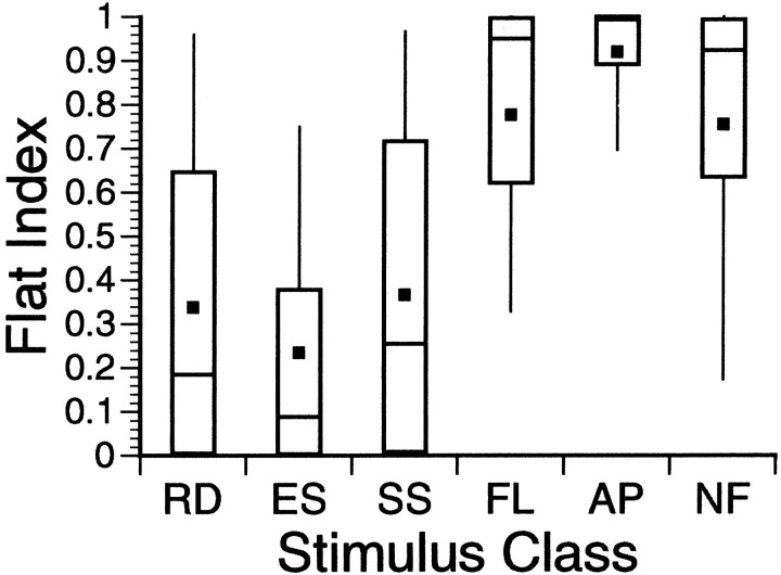
A total of 781 experiments was performed on these cells (639 on cells from monkey 90-2 and 142 from monkey 89-1). These broke down into stimulus classes as follows: 190 RD, 119 ES, 184 SS, 119 FL, 119 AP, and 50 NF. Many of these experiments were eliminated from further consideration here because of a lack of differential response to motion pattern type, as indicated by an FI of >0.95, leaving 158 (83%) RD, 116 (97%) ES, 152 (83%) SS, 57 (48%) FL, 36 (30%) AP, and 26 (52%) NF. The percentage of ES experiments passing this test is deceptively high compared with the RD and SS classes. This is because the RD and SS patterns were the only stimulus classes investigated in 89-1, and this monkey’s responses in MSTd were not as vigorous as those for 90-2. Although we have no good explanation for this, differences in visual acuity cannot be ruled out; neither monkey’s vision was tested. If only 90-2’s data are considered, the proportion of experiments that remained after FI screening for the RD and SS classes is near the 97% found for the ES class. Allowing for this, the six stimulus classes can be divided into two groups: a “vigorous response” group made up of the RD, ES, and SS classes and a “weak response” group made up of the remaining stimulus classes. This distinction is clear in Figure7, which looks at the distribution of FI by class.

Fig. 7.

FI distributions by class. This is a box plot showing the FI distributions by stimulus class. Each of the six plots should be viewed as a sort of compact histogram with a Gaussian-shaped distribution. The solid black squares indicate the distribution means. The short horizontal lines bisecting thevertical rectangles represent the medians of the distributions. The vertical rectangle includes 50% of all index scores. The “whiskers” attached to both ends of these rectangles extend out to include 80% of the data. The six stimulus classes fall fairly neatly into two different groups. The FL, AP, and NF classes, with high FI scores, are placed in a “poor responding” group. The remaining three classes gave more vigorous responses, as reflected in their lower FI distributions.

Data sets from experiments with an FI of <0.95 were fit to Gaussian curves, and the lack of fit for each experiment was calculated, as detailed above in Materials and Methods. The Gaussian model’s lack of fit was not statistically significant for any of the data sets examined. After calculating this same statistic on the data sets normalized for mean response rate (“flattening” the data) as outlined above, the GI (our measure of response strength) was calculated for each experiment. If this measure of response did not exceed 0.1, the experiment was discarded from further analysis. A 0.1 threshold value was chosen because it represents the point at which the raw data set and the flattened data fit the Gaussian model obtained through regression equally well.

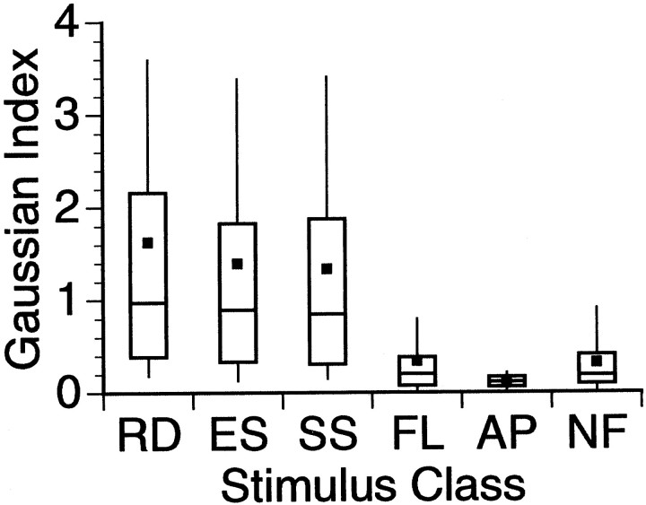
Figure 8 looks at the GI distribution as a function of stimulus class. The stimulus classes in order of increasing response strength are as follows: AP, FL, NF, ES, SS, RD. The separation of the stimulus classes into two groups based on response strength that was seen for the FI is also seen in this graph. The difference between the two stimulus groups is actually under-represented because of the disproportionate number of experiments in the poor responding group that were screened out before this round of analysis. If the FI screening hadn’t eliminated a substantial number of the FL, AP, and NF experiments, their distribution of GIs would have been shifted downward. Within these two groups, the responses were similar, although sometimes statistically different. Particularly interesting is the poor response of the FL stimulus compared with the SS, because the mean luminance contrasts and form for these two stimuli are identical. An examination of the significance of this follows in the Discussion. Table 1 presents a summary of the screening, showing the number of experiments for the six classes passing each round of elimination.

Fig. 8.

GI distribution by class. Graph is identical to that of Figure 7. The six stimulus classes fall fairly neatly into two different groups. The FL, AP, and NF classes, with low GI scores, are placed into the “poor responding” group, whereas the remaining three classes make up a “strong responding” category.

Table 1.

Number of experiments analyzed for each stimulus class at each round of screening

	# experiments	FI < 0.95	GI > 0.1	FI average	GI average
RD	190	158	156	0.34	1.63
ES	119	116	107	0.23	1.39
SS	184	152	143	0.37	1.33
FL	119	57	42	0.78	0.34
AP	119	36	23	0.92	0.11
NF	50	26	20	0.75	0.32

Numbers in the first column are the total number of experiments for which data was collected. Experiments were excluded from further consideration at two sequential stages. At the first stage, only those experiments with an FI <0.95 were regressed to a Gaussian model with subsequent calculation of a GI for that data. If an experiment’s GI was >0.1, it was used in future comparisons. The right two columns give averages of the FI and GI for all experiments in which they were calculated. The GIs for FL, AP, and NF classes would have been even lower had not a substantial number of these experiments been eliminated at the previous round.

The preceding screening procedure eliminated all experiments with nearly flat tuning curves. This strategy would exclude both experiments in which the cell did not respond to any of the motion types and experiments in which the cell responded nonselectively to the different motion types. To distinguish between these two possibilities for “flat” experiments, t tests comparing the responses to each motion type were compared against the background firing rate of the cell. The Bonferroni method for multiple t tests judged significance at the p < 0.05/8 = 0.00625 confidence level. Table 2 shows the six experimental classes broken down into three categories based on this test. “Tuned” experiments were experiments with GIs >0.1. “Untuned” experiments had GIs <0.1, but the neurons give a significant response to at least one motion type. Overall, 57% of the experiments with GIs <0.1 fell into the Untuned group. More than 95% of these significant responses represented an increase in firing above background. When we reexamined the raw data from the Untuned group, we confirmed that these experiments did not have well defined tuning curves, but instead had fundamentally flat responses with some sporadic activity.

Table 2.

Experiments by stimulus class and response category

	Tuned	Untuned	No Response
RD	156 /190	0 /190	34 /190
	(82%)	(0%)	(18%)
ES	107 /119	12 /119	0 /119
	(90%)	(10%)	(0%)
SS	143 /184	30 /184	11 /184
	(78%)	(16%)	(6%)
FL	42 /119	54 /119	23 /119
	(35%)	(45%)	(20%)
AP	23 /119	48 /119	48 /119
	(20%)	(40%)	(40%)
NF	20 /50	20 /50	10 /50
	(40%)	(40%)	(20%)

As explained in the text, tuned experiments are those with Gaussian indexes >0.1; Untuned and No Response experiments have GIs <0.1. With Untuned experiments, at least one motion type produced a significant response. The table includes the fraction of experiments in each group, followed by the percentage.

Figure 9 is a histogram that further breaks down the experiments in the Untuned group according to the number of motion types that gave responses significantly different from background. The bin with the largest number of experiments was “8:” for these experiments, all motion pattern types for a particular class gave significant responses. There were also a large number of experiments in which only a single motion type gave a significant response. Although most of the subsequent analysis will focus on the Tuned group of experiments, in a later section both the Untuned and No Response experiments will be analyzed using nonparametric techniques that do not require fitting tuning curves to specific functions.

Fig. 9.

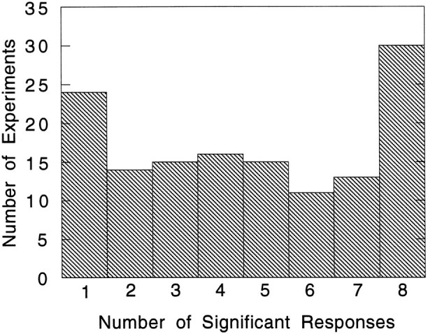
Histogram breaking down the Tuned category of experiments according to the number of motion types for each experiment producing a significant response. Note the large number of experiments for which multiple motion types produced a significant response.

Preferred stimulus pattern

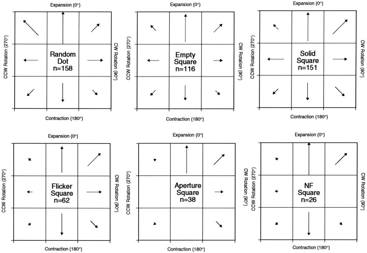
Figure 10 shows the distributions of the Gaussian mean parameters for each stimulus class. This parameter reflects the preferred stimulus type for the unit. The length of the vector in each box corresponds to the number of units with preferred tuning direction in that range. The boxes are arranged as per the representation of “spiral space” discussed above. As has been observed in other studies of area MSTd, there is a predominance of cells tuned for expansion. This was true across all stimulus classes. For the AP class, no units tuned to counterclockwise (CCW) rotation or contraction were found, and for the NF class, no cells were found tuned to clockwise (CW) rotation. This is likely a consequence of insufficient sampling because of the small number of units that gave sufficient responses to these stimulus classes.

Fig. 10.

Distribution of preferred tuning directions (Gaussian means) by stimulus class. An over-representation of units tuned to expansion is observed. A second, smaller peak for contraction is also evident. For this analysis, spiral space was divided into eight equally sized pieces, as shown in each of the six plots. These diagrams are organized in a similar manner to the polar plots in preceding figures. A response profile was characterized as being centered around “expansion,” for example, if the preferred tuning direction recovered for an experiment was between −22.5° (same as 337.5°) and 22.5°. Each box, representing one of the eight stimulus types, contains a vector, the orientation of which points in the direction of spiral space being considered, and the length of the vector reflects the number of units with this tuning preference. The inconsistencies with regard to the FL, AP, and NF classes are likely a consequence of small sample sizes.

Form/cue invariance across the MSTd cell population

In Figures 5 and 6, the form/cue invariance of a single MSTd neuron was documented. Based on our analysis of response strength, we can now show that this is a property of the MSTd cell population as a whole.

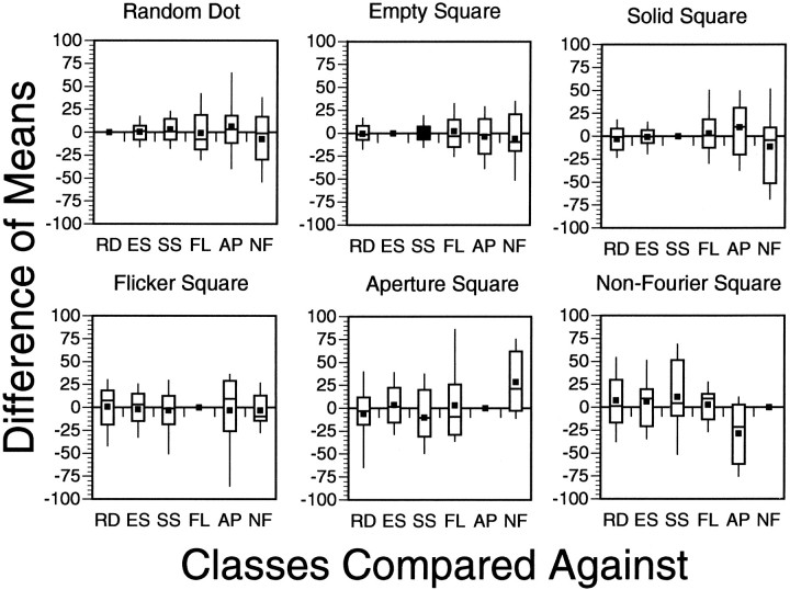
Pairwise analysis of a unit’s preferred tuning direction in spiral space with respect to each stimulus class was performed. All six stimulus classes (RD, ES, SS, FL, AP, and NF) were potentially considered, although in many cells the responses to some classes were not strong enough to make all possible pairs of comparisons. To quantify tuning invariance, we made pairwise comparisons of the Gaussian means. Fifteen unique (30 total) potential pairwise comparisons were possible between the different classes for a single unit. These comparisons, along with the number of comparisons made, are as follows: (RD vs ES: 105, RD vs SS: 126, RD vs FL: 35, RD vs AP: 18, RD vs NF: 19, ES vs SS: 93, ES vs FL: 32, ES vs AP: 17, ES vs NF: 19, SS vs FL: 31, SS vs AP: 16, SS vs NF: 17, FL vs AP: 10, FL vs NF: 9, AP vs NF: 2). Table 3 shows the percentage of cases for each comparison in which the fitted Gaussian means of the classes under consideration fell outside each other’s 95% confidence intervals. Table 4 shows the average difference in preferred tuning (taken as the absolute value of the pairwise subtraction of Gaussian means) between each of these stimulus classes. Clearly, those comparisons involving classes that gave poor responses tended to show larger average differences. Figure 11 is a series of box plots comparing the differences in these fitted means for each of the 15 comparisons. In each case, except for the comparison of AP and NF (where the N number is only 2), the difference is centered around zero. In no case was the difference between any two stimulus classes significantly different from zero (two-tailedt test, p < 0.05). More importantly, the range of values bracketed by the tips of the “whiskers” in these plots account for 80% of the variation in preferred tuning associated with stimulus class. Therefore, the preferred tuning directions established from different stimulus classes were generally within 30° of each other.

Table 3.

Percentage of preferred tuning directions statistically different between stimulus classes

	RD	ES	SS	FL	AP	NF
RD	xxx	14.3	23	34.3	16.7	36.9
ES	14.3	xxx	14	25	29.4	42.1
SS	23	14	xxx	25.9	37.5	47.1
FL	34.3	25	25.9	xxx	30	0
AP	16.7	29.4	37.5	30	xxx	0
NF	36.9	42.1	47.1	0	0	xxx

A particular comparison is represented by the intersection of a row and a column labeled with the classes being compared. Numbers are the percentage of instances in which the fitted means of two experiments’ tuning curves fell outside each other’s 95% confidence intervals obtained during regression. Only experiments in which both the GIs exceeded 0.1 were used for this comparison.

Table 4.

Average difference in preferred tuning by stimulus class (in degrees)

	RD	ES	SS	FL	AP	NF
RD	xxx	10.3	15.4	25.1	30.9	27.2
ES	10.3	xxx	10.6	20.2	21.3	25.5
SS	15.4	10.6	xxx	24.9	40	32.9
FL	25.1	20.2	24.9	xxx	31.9	16.7
AP	30.9	21.3	40	31.9	xxx	35.9
NF	27.2	25.4	32.9	16.7	35.9	xxx

This table is in the same format as Table 3. Numbers represent the average observed difference in preferred tuning direction between stimulus classes for individual units. Numbers are all positive because absolute values of these differences were taken. If feature invariance did not occur in MSTd, these averages would all be distributed at ∼90°. Thus, a considerable degree of invariance is indicated. Note that numbers are smaller when comparisons are made between classes that gave strong responses (RD, ES, SS).

Fig. 11.

Stimulus class differences in preferred tuning direction (population distribution). The form of these box plots is the same as in Figure 7. The title of each plot is a different stimulus class. The x-axis shows the class against which the title class is compared; the y-axis reflects the magnitude of these tuning differences. In the convention we have adopted, a positive difference indicates that the shift in preferred tuning from title class to x-axis class was clockwise, a negative difference counterclockwise. The sign of these differences has been preserved. Thefilled square represents the mean shift; the top,middle, and bottom horizontal lines through each vertical box correspond to the 75th percentile (top quartile), 50th percentile (median), and 25th percentile (bottom quartile), respectively. The whiskers on the topand bottom extend from the 10th percentile (bottom decile) to the 90th percentile (top decile). The comparison of one experimental type against itself is obviously zero, and these data are shown only for reference.

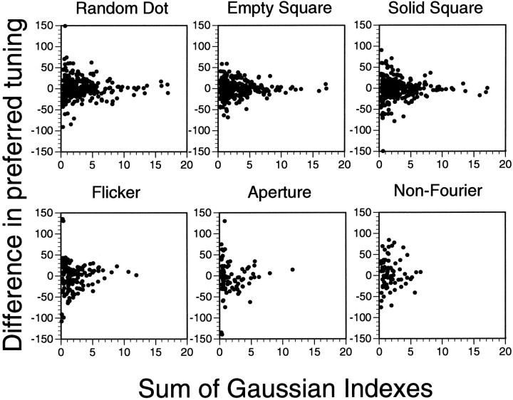
We postulated that any difference between preferred tuning directions was a consequence of noise in the data used to fit the curves. If this was the case, experiments in which the responses to the stimuli were more robust would be expected to have smaller differences between their preferred tuning directions. Figure 12 plots the magnitude of these tuning differences against the sum of the GIs of the two experiments compared. As discussed above, a total of 30 (15 unique) such comparisons are possible, each of the six stimulus classes being involved in 5 comparisons. (We are not considering comparing a stimulus class with itself, which obviously always has a difference of zero.) Note that the long axis of the “wedge”-shaped data are along thex-axis, indicating that the distribution is centered around zero. The variance associated with the difference in preferred tuning direction is large at small GI sums but small with high GIs. This is exactly what is expected with a stochastic distribution of the data around zero, with the GIs as a reflection of the randomness of the data. This correlation is consistent with invariance of preferred tuning direction across different stimulus classes.

Fig. 12.

Differences in preferred tuning direction versus GI sum. Based on the hypothesis that MSTd selectivity is invariant with regard to the form, feature, and class defining motion pattern, we predicted that any variation in preferred tuning between classes was largely a function of the inherent noisiness in cell response. Because the GI reflects response robustness, we predicted that differences in tuning would, on average, be smaller when calculated between experiments with high GIs. In this figure, by plotting the difference in preferred tuning against the sum of the GIs of the experiments compared, it can be seen that this is the case. For each plot, five types of potential comparisons are made, with the title of the plot indicating the stimulus class in common for each of these comparisons. For example, the graph at the upper left makes the comparisons RD–ES, RD–SS, RD–FL, RD–AP, and RD–NF.

Other model parameters

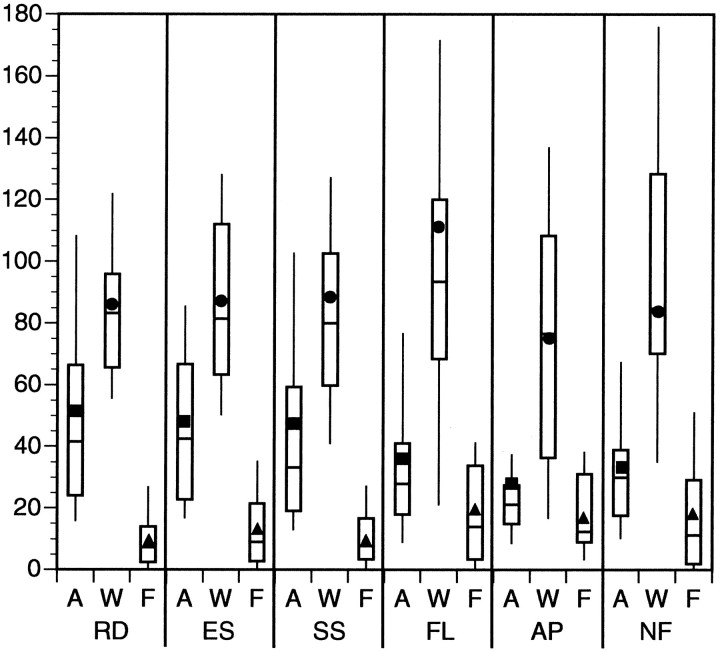
We also examined the relative magnitudes of the other three Gaussian parameters, i.e., amplitude (in spikes/sec), variance (in degrees of spiral space), and floor (in spikes/sec). The distribution of the amplitude parameter as a function of stimulus class is shown in Figure 13. Not surprisingly, this plot looks similar to Figure 8, which shows the distribution of GIs by class. Both response amplitude and GI reflect response strength. As has been seen previously, the six classes of response can be divided into strong responding and weak responding classes.

Fig. 13.

Box plots of response amplitude (in spikes/sec), width (in degrees), and floor (in spikes/sec) by stimulus class. The RD, ES, and SS classes consistently demonstrated larger response amplitudes than the other three classes. This diagram under-represents this trend because many nearly flat sets of data obtained from FL, AP, and NF classes were eliminated before this round of analysis. Response width is a measure of a unit’s selectivity for its preferred stimulus pattern. Higher values for this parameter indicate broader tuning curves. The distribution of this parameter was somewhat greater for the FL, AP, and NF classes, but the means of these distributions were similar. Response floor is a measure of a unit’s response to its anti-preferred stimulus pattern and is often close to the baseline firing rate of the neuron. An explanation for the slight upward shift in the distributions of the FL, AP, and NF classes is given in the text. A, Response amplitude; W, response width;F, response floor.

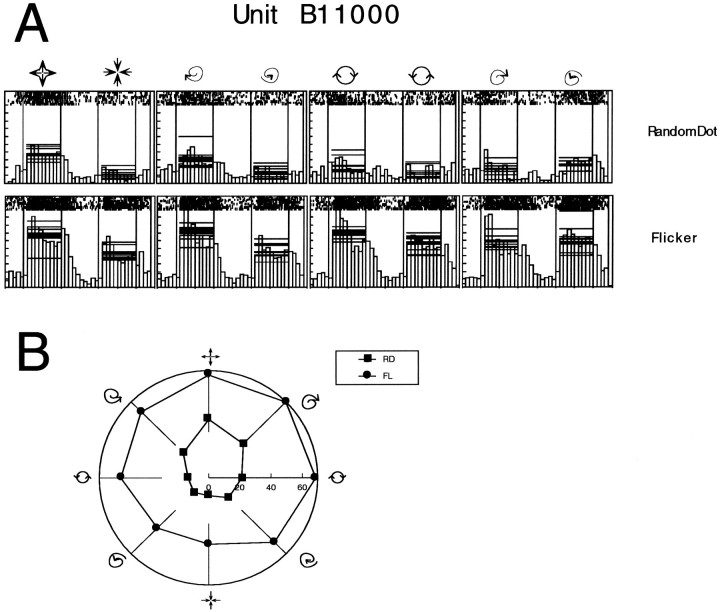
A similar analysis was performed for the variance (width) and the floor (estimate of firing rate in anti-preferred direction) in Figure 13. The data indicates that the width of the response curves is somewhat greater, on average, for the FL, AP, and NF classes, although this rarely reached statistical significance. However, the range of tuning widths is much greater for these classes. The magnitude of the floor parameter was, on average, greater for the three weak responding classes than for the strong responding classes. The difference only reached statistical significance when the FL class was compared with the RD, ES, and SS classes. A subpopulation of MSTd cells responded strongly to all types of motion pattern defined under the FL class, explaining the elevation of the floor parameter. An example of such a unit is shown in Figure 14, in which the responses to the FL and RD classes are compared. This tonic elevation in response was not observed in the majority of cases, and in a small number of cases the opposite effect—tonic inhibition—was observed. However, enough units responded like the cell in Figure 14 to significantly affect the average value of the floor for the FL class.

Fig. 14.

Responses of MSTd units to the FL stimulus class. For a subclass of neurons in this region, the response to the FL stimulus class was always well above the background firing rate of the cell, even for the anti-preferred tuning direction. A, Raw spike data and spike histograms for unit B11000. Pictures above the data represent the stimulus pattern that elicited the responses underneath. For each histogram, the horizontal lines represent the average activity to the stimulus for individual trials. The responses to the RD and FL classes are compared. For the FL class, note that both responses in the preferred and anti-preferred directions are shifted upward. B, Polar plot of this data, comparing the tuning curves.

Circular and nonparametric analysis

A potential shortcoming of the preceding analysis is that a substantial number of experiments with flat tuning curves were excluded at the first stage. This was done because flat tuning curves cannot be modeled after Gaussian functions. As noted above, ∼60% of experiments with flat tuning curves had responses that were significantly above the background firing rate of the cell. It is desirable to include these experiments in the analysis. In this section, we reanalyze all the data using nonparametric methods, which allows all the data to be compared and doesn’t require fitting the tuning curves to a particular model.

As explained in Materials and Methods, the trigonometric means for each experiment were calculated. For experiments with well tuned responses, these numbers agreed closely with the estimates of preferred tuning obtained through fitting Gaussian functions. Based on the nonparametric statistic discussed in Materials and Methods, pairwise comparisons of preferred tuning were made between classes for each neuron. Table5 shows the frequency with which these estimates of preferred tuning varied between experimental classes. This table follows the same format as Table 3, when this same comparison was performed on the screened set of data with parametric methods. Unlike Table 3, Table 5 includes comparisons of experiments with flat responses and consequently large degrees of uncertainty surrounding the estimation of preferred tuning.

Table 5.

Frequency at which different stimulus classes produced significantly different preferred tuning in the same neuron (circular statistics)

	RD	ES	SS	FL	AP	NF
RD	xxx	10/119	23/184	12/119	16/119	14/50
		(8.4%)	(12.5%)	(10.0%)	(13.4%)	(28.0%)
ES	10/119	xxx	8/119	7/119	17/119	12/50
	(8.4%)		(6.7%)	(5.9%)	(14.2%)	(24.0%)
SS	23/184	8/119	xxx	7/116	16/116	18/47
	(12.5%)	(6.7%)		(6.0%)	(13.7%)	(38.3%)
FL	12/119	7/119	7/116	xxx	9/119	5/50
	(10.0%)	(5.9%)	(6.0%)		(7.6%)	(10.0%)
AP	16/119	17/119	16/116	9/119	xxx	7/50
	(13.4%)	(14.2%)	(13.7%)	(7.6%)		(14.0%)
NF	14/50	12/50	18/47	5/50	7/50	xxx
	(28.0%)	(24.0%)	(38.3%)	(10.0%)	(14.0%)

This information is the same as that presented in Table 3, except that these comparisons used nonparametric statistics and compared all experiments for which data was collected.

Previously, only pairwise comparisons of preferred tuning were made on the data. Also of interest to compare across classes is the selectivity (width) of the responses. Because previously the screening step preferentially excluded experiments with broad selectivity, pairwise comparisons of the remaining experiments would be unavoidably biased. To overcome this problem, the sample circular variance, a nonparametric index from circular statistics (see Materials and Methods), was calculated for each experiment. This measure of responses selectivity can be obtained from experiments even with poor selectivity. A perfectly tuned neuron—one that fired only in response to the preferred stimulus—is defined as having a circular variance of “0.” At the other extreme, a circular variance of “1” describes a perfectly nonselective cell, in which the neuronal firing rate is the same for all motion types.

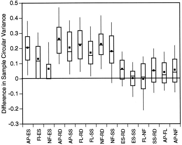
Figure 15 presents 15 bar plots showing the population distributions of pairwise differences in circular variance. (With 6 different stimulus classes there are 15 unique comparisons.) This figure follows the same conventions as the previous bar plots. This figure shows that for a particular cell, responses from AP, FL, and NF classes were consistently less selective than for the RD, ES, and SS classes. In addition, comparisons within the RD, ES, and SS classes, as well as within the AP, NF, and FL classes, were centered around zero.

Fig. 15.

Box plot showing distribution of differences in circular variance obtained from pairwise stimulus class comparisons. The first nine comparisons along the x-axis show circular variance differences between classes of different response types (weak responding vs strong responding). Last six box plots show comparisons between classes of the same response type.

This information is summarized in Table 6, which breaks down the data from each class into the Tuned, Untuned, and No Response categories discussed above, followed by an “all” row that pools this information. The last three rows pool data from all six classes together for each response category. This table also summarizes additional descriptive statistics such as average firing rate, obtained by determining average firing rate summed across the eight motion types. Because background firing rate did not vary across stimulus classes or response categories, this index reflects overall responsiveness to each stimulus class. In general, the Tuned and Untuned experiments had similar average firing rates, and experiments that fell into the No Response category had weak responses. Therefore, the difference between the Tuned and Untuned experiments was with respect to the selectivity and not the magnitude of the response.

Table 6.

Summary of nonparametric indexes broken down into stimulus class and response type

	n	Average firing rate	% sig resp. (Rayleigh)	Circular variance	Directional index
RD (Tuned)	156	30	90	0.59	0.78
RD (Untuned)	0	—	—	—	—
RD (No Response)	34	10	15	0.73	0.57
RD (All)	190	27	82	0.61	0.74
ES (Tuned)	107	33	87	0.63	0.73
ES (Untuned)	12	46	20	0.82	0.45
ES (No Response)	0	—	—	—	—
ES (All)	119	34	81	0.64	0.70
SS (Tuned)	143	28	87	0.64	0.73
SS (Untuned)	30	37	0	0.83	0.43
SS (No Response)	11	13	0	0.80	0.57
SS (All)	184	26	74	0.67	0.68
FL (Tuned)	42	35	63	0.74	0.58
FL (Untuned)	54	33	11	0.87	0.33
FL (No Response)	23	12	38	0.75	0.47
FL (All)	119	30	33	0.81	0.44
AP (Tuned)	23	26	50	0.77	0.53
AP (Untuned)	48	24	11	0.88	0.38
AP (No Response)	48	13	7	0.86	0.41
AP (All)	119	20	17	0.85	0.42
NF (Tuned)	20	30	56	0.71	0.63
NF (Untuned)	20	24	20	0.83	0.42
NF (No Response)	10	12	23	0.82	0.38
NF (All)	50	23	32	0.79	0.48
All classes (Tuned)	491	31	83	0.63	0.72
All classes (Untuned)	164	30	13	0.86	0.38
All classes (No Response)	126	13	17	0.82	0.43

The table represents the average value of the appropriate index (column) for the appropriate set of experiments (row). Average firing rate sums responses for each experiment across all eight motion types. The Rayleigh test is a circular, nonparametric statistic for uniformity of response across motion type. The circular variance reflects response width and has a range of 0–1. A circular variance of 1 describes a perfectly uniform response. The directional index is a measure of response strength obtained by comparing preferred and antipreferred response rates. The antipreferred direction is defined as the motion type 180° (in spiral space) from the direction of maximum response.

Another statistic summarized in Table 6 is the Rayleigh test for nonuniformity (see Materials and Methods). The table shows the percentage of experiments in each group whose responses varied significantly from a uniform distribution. As expected, this nonparametric test showed that a high percentage of Tuned experiments had nonuniform responses.

A conventional directional index (1 − antipreferred response/preferred response) was calculated for each experiment, and the results are summarized in the final column of Table 6. The RD class, on average, produced experiments with the highest directional indexes (most Tuned responses) followed by the ES and SS classes. As expected, the FL, AP, and NF classes gave less directional responses. The Untuned and No Response experiments gave less directional responses than the Tuned experiments.

Positional invariance

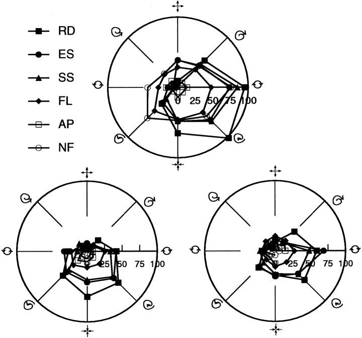
For a few cells that we were able to hold for an extended period of time, the battery of experiments was repeated with the stimuli positioned at different locations in the unit’s receptive field. The property of positional invariance with respect to preferred tuning has been noted in several labs, including our own (Graziano et al., 1994). In this previous investigation, units were tested for this property over ranges of only 10–20° because of limitations in the display device. The large screen used in this study allowed us to position the stimuli over much larger differences in visual angle. Because MSTd receptive fields can be quite large, in some cases the center of the stimulus could be moved as far as 50° and still elicit a strong response.

Figure 16 shows one such case, in which both positional and form/cue invariance were simultaneously tested in the same unit. Data were separately collected with the stimuli centered in three regions of the neuron’s receptive field. These three locations formed the apexes of an equilateral triangle, with each corner 50° of visual angle away from the other two. In each location, tuning curves for all six stimulus classes were obtained. To a large extent, stimulus specificity in terms of preferred stimulus type was maintained, independent of both stimulus class and location.

Fig. 16.

Three sets of polar plots showing tuning response invariance with respect to both stimulus feature and location within the receptive field. These data were recorded from a cell (B11300) with a particularly large receptive field. This allowed for placement of the stimuli at three spatial locations each 50° apart from one another, forming the corners of an equilateral triangle. Data from each polar plot was obtained from a different spatial location. Although response amplitude varied considerably over feature classes and stimulus location, the overall orientations and widths of these 18 tuning curves were remarkably similar. Some shift in preferred tuning is noticed with stimulus location, but this is generally small considering the large displacements involved.

DISCUSSION

This study has demonstrated form/cue invariance in macaque area MSTd, supporting the hypothesis that this region generically represents motion patterns, such as those projected onto the retina by moving objects and observer self-motion. Earlier workers in MSTd made preliminary observations with regard to texture and shape invariance in MSTd tuning (Sakata et al., 1985, 1986; Tanaka et al., 1986, 1989). These studies showed that manipulating qualities of the stimulus, such as contrast polarity (Saito et al., 1986) and texture, somewhat affected the amplitude of the response, but had little effect on overall selectivity for motion pattern. It has also been demonstrated that, unlike the case for translational motion, selectivity for expansion, contraction, and rotation is independent of stimulus size and speed (Duffy and Wurtz, 1991b).

Recent progress in our understanding of MSTd response properties allowed us to explore form/cue invariance further. At the time of the previous investigations, the conceptual framework of “spiral” space had yet to be introduced, and the smooth continuity of motion pattern selectivity between expansion and contraction was not recognized. As a consequence, the tuning curves constructed in the current study, which recover fairly precise estimates of preferred tuning, were not available. Previously, cells were characterized as being selective for expansion, contraction, rotation, or some combination of these motion types, rather than assigned a direction in spiral space. As a consequence of this coarse characterization, it is not possible to adequately assess the degree of tuning invariance, because changes in response strength and preferred tuning are confounded (Graziano et al., 1994). By evenly sampling spiral space with eight stimuli located 45° apart in this space (8 × 45 = 360) and fitting the differential responses elicited by these stimuli to a Gaussian function, preferred tuning direction can often be confidently recovered to within a few degrees. This allows us to quantify more subtle shifts in tuning across stimulus class and stimulus location (Graziano et al., 1994). The second limitation of the earlier studies was the choice of stimulus classes. The range of features and cues in the current investigation are much more diverse than those of previous work.

Neural coding

Our definition of form/cue invariance only extends to a unit’s preferred stimulus pattern and does not consider either response strength or width. Although we believe that this formulation is well grounded, it relies on assumptions about neural coding and the construction of our tuning curves that we should make explicit.

The general Gaussian function with four parameters (mean, width, amplitude, and floor) was used to fit the tuning curves from each experiment. This function fits the data sets well, and its four unknowns can be directly related to important aspects of the response profile.

The Gaussian mean recovers the motion pattern type to which a neuron most vigorously responds. Average firing rate was our only criteria for establishing “preferred tuning”—more subtle encoding strategies such as the temporal firing pattern were not considered. Preferred tuning is important because the motion pattern presented to the monkey is assumed to be encoded in the MSTd population response profile. For example, if neurons tuned to expansion fire at a higher rate than any other population of neurons, presumably the monkey is perceiving expansion motion.

Whereas the mean of the Gaussian model is intimately related to the type of motion pattern being represented, the width (variance) of the Gaussian may be related to discriminability. A subject’s ability to discriminate motion direction is correlated with the maximum slope of area MT tuning curves, a parameter inversely related to the width of the Gaussian response profile (Snowden et al., 1992). Further work needs to be done to establish whether there is a direct correlation between pattern motion discrimination and tuning curve width in MSTd.

The Gaussian amplitude parameter (which reflects a unit’s response to the preferred stimulus pattern) could reflect both stimulus saliency and stimulus location. Increasing the saliency of a stimulus, for example by increasing stimulus contrast, generally leads to more vigorous responses in neurons specific for these patterns (Barlow et al., 1987). Whereas increasing saliency leads to a general increase in responses across an entire cortical area, shifting the location of a stimulus increases responses in some units and decreases responses in others. Stimulus location thus could be represented in the relative activities of different populations of cells with the same specificity but with receptive fields covering different areas of the visual field.

Finally, the Gaussian floor parameter (which reflects a unit’s response to the anti-preferred stimulus pattern) also may be affected by stimulus saliency. Traditional measures of response strength use comparison operations between the preferred and anti-preferred responses. Therefore, for a given Gaussian amplitude, a lower response floor may reflect greater stimulus saliency.

Positional invariance

In the above conception of neural coding, only the direction of the preferred response (in spiral space) is related to the type of motion pattern represented. In our previous work in MSTd (Graziano et al., 1994), we considered a unit’s response as positionally invariant if its preferred tuning did not shift after moving the stimulus pattern within the neuron’s receptive field. Other characteristics of the response profile (width, amplitude, and floor) did not exhibit the same degree of invariance. For example, near the edge of the receptive field, it is typical for the response amplitude to gradually fall off, despite the preferred tuning direction remaining unchanged. Invariance in preferred tuning is important because it means that a population of cells has the same response profile, regardless of where the stimulus is placed in the animal’s visual field. Given the model of neural coding presented above, this response characteristic could account for the perceptual invariance experienced when placing these patterns at different locations within the visual field; i.e., the perception of a pattern such as expansion is independent of its location in the visual scene.

This idea is not new. Desimone et al. (1984) found a similar positional invariance in area IT with respect to spatial patterns. Analogous to our observations in area MSTd, the invariance did not extend to the amplitude of the response, which was reduced at the edges of the receptive field.

Recently, Duffy and Wurtz (1995) reported that the amplitude of the response to the preferred stimulus often changes with stimulus placement in MSTd. This interesting finding provides a way for stimulus location to be encoded by a population of cells through coarse coding, a possibility also proposed by Graziano et al. (1994). The ability to recover the location of the focus of outflow in elementary flow patterns is likely important if MSTd provides DOH processing. However, we believe these amplitude changes only encode stimulus location within the receptive field and are unrelated to the type of pattern being represented. Although Duffy and Wurtz (1995) acknowledge the tuning invariance of many MSTd cells, they make a distinction between “relative” and “absolute” invariance. They qualify our finding of positional invariance, claiming that MSTd cells demonstrate only “relative” invariance because large shifts in stimulus placement produce significant changes in the amplitude of the response to the preferred stimulus. “Absolute” invariance requires that the amplitude of the response to the preferred stimulus type remain unchanged despite shifting the stimulus location by large amounts (e.g., 40°). This distinction is potentially misleading because our conception of invariance does not extend to response amplitude, but depends only on the motion pattern giving the strongest response. For reasons discussed above, we believe preferred tuning is a more relevant measure of invariance than the neuron’s response amplitude to a single stimulus pattern.

Form/cue invariance

In the present study, rather than shifting the stimulus within a unit’s receptive field, the features and cues used to define the motion pattern were changed, and the tuning curves were compared. Invariance is again interpreted as no change in preferred tuning. The stimulus classes tested clearly differed in their perceptual saliency, and we believe this is reflected in the width, amplitude, and floor parameters of the tuning curves. As in our previous study on positional invariance, what remains unchanged is the motion pattern providing the strongest response. As discussed above, this invariance provides a mechanism for extracting a pure motion pattern signal from a stimulus containing other properties such as location, shape, size, color, and form.

Our experiments indicate that the preferred motion pattern for a majority of cells in area MSTd is not dependent on the features that define the motion. When statistically significant differences in preferred tuning existed, the magnitude of these differences tended to be small compared with the possible range of preferred tunings. As a population, the more confident we were with the Gaussian models we obtained from the data, the smaller these differences were.

In our laboratory’s previous paper on MSTd, we introduced an analogy with area IT (Graziano et al., 1994). Area IT has long been thought to represent the spatial organization of stimulus features. It is sensitive to stimulus attributes that MSTd ignores, i.e., shape and form. In this region, investigators have reported the existence of “face cells,” “toilet brush cells,” and the like (Gross et al., 1972). In contrast, we have discussed evidence that a specificity for motion pattern exists in MSTd.

Reinforcing the analogy of IT with MSTd, cue invariance has been reported in area IT as well (Sary et al., 1993). These investigators recognized that the perception of shape is invariant with respect to location in space, size, and the cues that define the shape. Using cues based on differences in luminance, motion, and texture, they found in IT a physiological correlate of this perceptual invariance: the neurons ignored aspects of the stimulus unrelated to spatial structure. The outputs of IT and MSTd converge in the anterior STS and part of the posterior parietal cortex, perhaps to pool together information from these different processing streams.

Form/cue invariance has been demonstrated in other visual areas. Single-unit recording studies in area V1 of the macaque have demonstrated form/cue invariance in selectivity for image contours (Albright and Chaudhuri, 1989) and in MT for local translational motion signals (Albright, 1992). This independence held for band width and preferred tuning, but not for response amplitude. In these studies, the average difference in preferred tuning direction did not vary from zero, and no more than 30 percent of the differences were outside the range of ±45°. This is similar to our findings in MSTd for motion pattern. These authors suggested, as we have, that amplitude is related to attribute saliency.

The repeated finding of form/cue invariance in IT, MT, MSTd, and other areas of the brain is likely because of the computational efficiency it affords. As an analogy, consider the system of mathematics. We have one set of rules to manipulate any kind of quantity, whether it be number of dogs, birds, or golf balls. The numerical computations performed on these things do not depend on what the numbers are representing. If the brain had a separate system for the motion analysis of squares, circles, triangles, and what not, the brain would be prohibitively large. By breaking any analysis down into separate parts, great redundancy is avoided.

In this conception, perceptual systems are segmented into distinct processing channels. There are regions of the brain specialized for processing stimulus attributes such as motion, color, and form. It is the combination of activities from each of these areas that determines the unified perception of the world. By having these channels as independent as possible, we not only reduce redundancy, but prevent interference between processes that need to remain distinct.

Response strength and stimulus class

From our data, it is evident that the stimulus classes RD, ES, and SS gave more tuned responses than FL, AP, and NF (Figs. 7, 8). This was confirmed by our nonparametric analysis of the entire data set, which showed greater selectivity for the RD, ES, and SS classes. The differences in response strength may reflect differences in stimulus saliency and/or discriminability. Although additional psychophysics needs to be done to confirm this, casual observation of the stimuli suggests that the RD, SS, and ES classes are more salient than the AP and NF classes. In contrast, the perceptual saliency of the FL class is greater than what would be predicted based on the population response in MSTd to these patterns. Although the population response was weak, a subpopulation of MSTd cells gave robust responses to this stimulus class (data not shown), possibly accounting for the high perceptual saliency.

Snowden et al. (1991) showed that the introduction of flickering or stationary random dots suppressed the response of MT cells to motion. Consistent with this finding, the poor response to the AP class is likely a consequence of the stationary features within the interiors of these patterns. Similarly, the flicker in the interior of the FL class likely inhibits the motion signals present at the edges of the square pattern.

Weak responses were observed for the NF class. Albright (1992) reported that the response in MT to NF patterns was approximately half that obtained with luminance-defined motion. In MSTd, responses to NF squares were much less than half as strong as responses to luminance squares. This difference may be related to the increased suppression of flicker in MSTd compared with MT (Lagae et al., 1994). It is likely that much of the second-order motion signal is lost in the smoothing that accompanies suppression of the flicker at the NF motion borders.

Optical flow versus object motion

MSTd units respond in a tuned manner to the types of motion pattern involved in both object motion and ego-motion perception. The form/cue invariance displayed by neurons in this region would facilitate both of these functions. Both types of processing require that the nervous system ignore the features and cues that define the patterns and extract only the motion signals.

One group (Tanaka and Saito, 1989) obtained poor responses in area MSTd using stimuli smaller than 20°. This would seem to make MSTd an unlikely candidate for the analysis of object motion because objects rarely subtend this large a visual angle. These earlier results are likely a consequence of recording under anesthetized conditions. Working with the awake, behaving monkey, we have recorded brisk responses using stimuli as small as 5° in diameter (our unpublished observation). Stimuli even smaller than this may potentially drive units if the monkey is trained to attend to these patterns, such as in a discrimination task. The presence of “rotation in depth” (rotation about the axis orthogonal to the line of sight) units reported by some workers (Sakata et al., 1985) offers further support for a motion pattern theory, as this type of motion pattern cannot be produced by self-translation in a stationary environment.

There is also evidence that optical flow information is processed in this region. As discussed above, the RD class of stimuli is inconsistent with the motion of a single rigid object, but these patterns are good approximations of optical flow patterns. The well tuned responses to these patterns argues in favor of MSTd processing optical flow information, potentially for ego-motion. The smooth pursuit eye signal found in area MSTd also supports a role for this region in ego-motion representation. A convergence of optical flow and smooth pursuit signals is believed to be important in recovering DOH (Warren and Hannon, 1988, 1990; Royden et al., 1992).

Many authors have emphasized the importance of being able to separately extract object and self-motion information (Swanston et al., 1987;Hildreth, 1991). For example, a baseball player running to catch a ball needs to isolate the motion of the baseball from all the retinal motion produced by his own movement. We propose that in area MSTd this information coexists and the parsing of the motion signals is delegated to other cortical areas or via attentional segregation within MSTd. In support of at least partial coprocessing for object and self-motion, it has been demonstrated that the motion of objects over optical flow patterns can influence the perceived location of the focus of expansion under some conditions (Royden and Hildreth, 1994; Warren and Saunders, 1994, 1995).

Several authors have proposed models exploring how area MSTd may extract DOH information from optical flow (Heeger and Jepson, 1992;Lappe and Rauschecker, 1993; Perrone and Stone, 1994). The results of the current study have little to say about the appropriateness of these models. These algorithms generally assume input from motion detectors modeled after MT cell responses. Given that the form/cues tested in this study all have been shown to effectively drive MT neurons, these stimuli should all provide appropriate input for DOH computations. Form/cue invariance in area MSTd is significant in that this property would be important for an area that needs to extract DOH under a wide variety of environmental layouts. Although form/cue invariance likely is established before reaching area MSTd, the position and scale invariance previously documented in this region (Graziano et al., 1994) requires elaborate specificity of connections between areas MT and MSTd.

Given the responses to the various square patterns observed, we believe the results of this investigation favor a direct role for area MSTd in the processing of object motion. The strong response to pure velocity fields in the case of the RD class also reinforces a role for this region in processing “optical flow”-related information. In either case, the form/cue invariance we report is important for both of these functions. It is prudent at this juncture to characterize MSTd as a generic “pattern motion” integration center.

REFERENCES

- 1.Albright TD. Direction and orientation selectivity of neurons in visual area MT of the macaque. J Neurophysiol. 1984;52:1106–1130. doi: 10.1152/jn.1984.52.6.1106. [DOI] [PubMed] [Google Scholar]
- 2.Albright TD. Form-cue invariant motion processing in primate visual cortex. Science. 1992;28:1141–1143. doi: 10.1126/science.1546317. [DOI] [PubMed] [Google Scholar]
- 3.Albright TD, Chaudhuri A. Orientation selective responses to motion contrast boundaries in macaque VI. Soc Neurosci Abstr. 1989;15:323. [Google Scholar]
- 4.Andersen GJ. Perception of self-motion: psychophysical and computational approaches. Psychol Bull. 1986;99:52–65. [PubMed] [Google Scholar]
- 5.Barlow HB, Kaushal TP, Hawken M, Parker AJ. Human contrast discrimination and the threshold of cortical neurons. J Opt Soc Am. 1987;4:2366–2371. doi: 10.1364/josaa.4.002366. [DOI] [PubMed] [Google Scholar]
- 6.Desimone R, Ungerleider LG. Multiple visual areas in the caudal superior temporal sulcus of the macaque. J Comp Neurol. 1986;248:164–189. doi: 10.1002/cne.902480203. [DOI] [PMC free article] [PubMed] [Google Scholar]
- 7.Desimone R, Albright TD, Gross CG, Bruce CJ. Stimulus selective properties of inferior temporal neurons in the macaque. J Neurosci. 1984;4:2051–2062. doi: 10.1523/JNEUROSCI.04-08-02051.1984. [DOI] [PMC free article] [PubMed] [Google Scholar]
- 8.DeYoe EA, Van Essen DC. Concurrent processing streams in monkey visual cortex. Trends Neurosci. 1988;11:219–226. doi: 10.1016/0166-2236(88)90130-0. [DOI] [PubMed] [Google Scholar]
- 9.Dittrich WH. Action categories and the perception of biological motion. Perception. 1993;22:15–22. doi: 10.1068/p220015. [DOI] [PubMed] [Google Scholar]
- 10.Drew T, Doucet S. Application of circular statistics to the study of neuronal discharge during locomotion. J Neurosci Methods. 1991;38:171–181. doi: 10.1016/0165-0270(91)90167-x. [DOI] [PubMed] [Google Scholar]
- 11.Duffy CJ, Wurtz RH. Sensitivity of MSTd neurons to optic flow stimuli. I. A continuum of response selectivity to large-field stimuli. J Neurophysiol. 1991a;65:1329–1345. doi: 10.1152/jn.1991.65.6.1329. [DOI] [PubMed] [Google Scholar]
- 12.Duffy CJ, Wurtz RH. Sensitivity of MSTd neurons to optic flow stimuli. II. Mechanisms of response selectivity revealed by small-field stimuli. J Neurophysiol. 1991b;65:1346–1359. doi: 10.1152/jn.1991.65.6.1346. [DOI] [PubMed] [Google Scholar]
- 13.Duffy CJ, Wurtz RH. Response of monkey MSTd neurons to optic flow stimuli with shifted centers of motion. J Neurosci. 1995;15:5192–5208. doi: 10.1523/JNEUROSCI.15-07-05192.1995. [DOI] [PMC free article] [PubMed] [Google Scholar]
- 14.Fisher NI. Cambridge UP; Cambridge: 1993. Statistical analysis of circular data. [Google Scholar]
- 15.Gibson JJ. Houghton Mifflin; Boston: 1950. The perception of the visual world. . [Google Scholar]
- 16.Graziano MSA, Andersen RA, Snowden RJ. Tuning of MSTd Neurons to Spiral Motions. J Neurosci. 1994;14:54–67. doi: 10.1523/JNEUROSCI.14-01-00054.1994. [DOI] [PMC free article] [PubMed] [Google Scholar]
- 17.Gross CG, Rocha-Miranda CE, Bender DB. Visual properties of neurons in inferotemporal cortex of the macaque. J Physiol (Lond) 1972;35:96–111. doi: 10.1152/jn.1972.35.1.96. [DOI] [PubMed] [Google Scholar]
- 18.Heeger DJ, Jepson AD. Subspace methods for recovering rigid motion I: Algorithm and implmentation. Int J Comput Vis. 1992;7:95–177. [Google Scholar]
- 19.Hildreth EC. Recovering heading for visually guided navigation. Vision Res. 1991;32:1177–1192. doi: 10.1016/0042-6989(92)90020-j. [DOI] [PubMed] [Google Scholar]
- 20.Hoffman DD, Flinchbaugh BE. The interpretation of biological motion. Biol Cybern. 1982;42:195–204. doi: 10.1007/BF00340076. [DOI] [PubMed] [Google Scholar]
- 21.Komatsu H, Wurtz RH. Relation of cortical areas MT and MST to pursuit eye movements. III. Interaction with full-field visual stimulation. J Neurophysiol. 1988;60:621–644. doi: 10.1152/jn.1988.60.2.621. [DOI] [PubMed] [Google Scholar]
- 22.Lagae L, Maes H, Raiguel S, Xiao DK, Orban GA. Responses of macaque STS neurons to optic flow components: a comparison of areas MT and MST. J Neurophysiol. 1994;71:1597–1626. doi: 10.1152/jn.1994.71.5.1597. [DOI] [PubMed] [Google Scholar]
- 23.Lappe M, Rauschecker JP. A neural network for the processing of optic flow from ego-motion in man and higher mammals. Neural Comput. 1993;5:374–391. [Google Scholar]
- 24.Mather G, West S. Recognition of animal locomotion from dynamic point-light displays. Perception. 1993;22:759–766. doi: 10.1068/p220759. [DOI] [PubMed] [Google Scholar]
- 25.Mather G, Radford K, West S. Low-level visual processing of biological motion. Proc R Soc London [Biol] 1992;249:149–155. doi: 10.1098/rspb.1992.0097. [DOI] [PubMed] [Google Scholar]
- 26.Maunsell J, Van Essen DC. Functional properties of neurons in middle temporal visual area of the macaque monkey. I. Selectivity for stimulus direction, speed, and orientation. J Neurophysiol. 1983a;49:1127–1147. doi: 10.1152/jn.1983.49.5.1127. [DOI] [PubMed] [Google Scholar]
- 27.Maunsell J, Van Essen DC. Functional properties of neurons in middle temporal visual area of the macaque monkey. II. Binocular interactions and sensitivity to binocular disparity. J Neurophysiol. 1983b;49:1148–1167. doi: 10.1152/jn.1983.49.5.1148. [DOI] [PubMed] [Google Scholar]
- 28.Nakayama K. Biological image motion processing: a review. Vision Res. 1985;25:625–660. doi: 10.1016/0042-6989(85)90171-3. [DOI] [PubMed] [Google Scholar]
- 29.Perrone JA, Stone LS. A model of self-motion estimation within primate extrastriate visual cortex. Vision Res. 1994;43:2917–2938. doi: 10.1016/0042-6989(94)90060-4. [DOI] [PubMed] [Google Scholar]
- 30.Poizner H, Bellugi U. Perception of American sign language in dynamic point-light displays. J Exp Psychol Hum Percept Perform. 1981;7:430–440. doi: 10.1037//0096-1523.7.2.430. [DOI] [PubMed] [Google Scholar]
- 31.Prazdny K. Egomotion and relative depth map from optical flow. Biol Cybern. 1980;36:87–102. doi: 10.1007/BF00361077. [DOI] [PubMed] [Google Scholar]
- 32.Royden CS, Hildreth EC. The effects of moving objects on heading perception. ARVO Abstracts. 1994;35:3440. [Google Scholar]
- 33.Royden CS, Banks MS, Crowell JA. The perception of heading during eye movements. Nature. 1992;360:583–585. doi: 10.1038/360583a0. [DOI] [PubMed] [Google Scholar]
- 34.Saito H, Yukie M, Tanaka K, Hikosaka K, Fukada Y, Iwai E. Integration of direction signals of image motion in the superior temporal sulcus of the macaque monkey. J Neurosci. 1986;6:145–157. doi: 10.1523/JNEUROSCI.06-01-00145.1986. [DOI] [PMC free article] [PubMed] [Google Scholar]
- 35.Sakata H, Shibutani H, Kawano K, Harrington TL. Neural mechanisms of space vision in the parietal association cortex of the monkey. Vision Res. 1985;25:453–463. doi: 10.1016/0042-6989(85)90070-7. [DOI] [PubMed] [Google Scholar]
- 36.Sakata H, Shibutani H, Ito Y, Tsurugai K. Parietal cortical neurons responding to rotary movement of visual stimulus in space. Exp Brain Res. 1986;61:658–663. doi: 10.1007/BF00237594. [DOI] [PubMed] [Google Scholar]
- 37.Sary G, Vogels R, Orban GA. Cue-invariant shape selectivity of macaque inferior temporal neurons. Science. 1993;260:995–997. doi: 10.1126/science.8493538. [DOI] [PubMed] [Google Scholar]
- 38.Schwartz EL, Desimone R, Albright TD, Gross C. Shape recognition and inferior parietal neurons. Proc Natl Acad Sci USA. 1983;80:5776–5778. doi: 10.1073/pnas.80.18.5776. [DOI] [PMC free article] [PubMed] [Google Scholar]
- 39.Simmons PJ, Rind FC. Orthopteran DCMD neuron: a reevaluation of responses to moving objects. II. Critical cues for detecting approaching objects. J Neurophysiol. 1992;68:1667–1682. doi: 10.1152/jn.1992.68.5.1667. [DOI] [PubMed] [Google Scholar]
- 40.Snedecor GW, Cochran WG (1989) Statistical methods. Iowa State UP.
- 41.Snowden RJ, Treue S, Erickson RG, Andersen RA. The response of area MT and V1 neurons to transparent motion. J Neurosci. 1991;11:2768–2785. doi: 10.1523/JNEUROSCI.11-09-02768.1991. [DOI] [PMC free article] [PubMed] [Google Scholar]
- 42.Snowden RJ, Treue S, Andersen RA. The response of neurons in areas V1 and MT of the alert monkey to moving random dot patterns. Exp Brain Res. 1992;88:389–400. doi: 10.1007/BF02259114. [DOI] [PubMed] [Google Scholar]
- 43.Swanston MT, Wade NJ, Day RH. The representation of uniform motion in vision. Perception. 1987;16:143–159. doi: 10.1068/p160143. [DOI] [PubMed] [Google Scholar]
- 44.Tanaka K, Saito H. Analysis of motion of the visual field by direction, expansion/contraction, and rotation cells clustered in the dorsal part of the medial superior temporal area of the macaque monkey. J Neurophysiol. 1989;62:626–641. doi: 10.1152/jn.1989.62.3.626. [DOI] [PubMed] [Google Scholar]
- 45.Tanaka K, Hikosaka K, Saito H, Yukie M, Fukada Y, Iwai E. Analysis of local and wide-field movements in the superior temporal visual areas of the macaque monkey. J Neurosci. 1986;6:134–144. doi: 10.1523/JNEUROSCI.06-01-00134.1986. [DOI] [PMC free article] [PubMed] [Google Scholar]
- 46.Tanaka K, Fukada Y, Saito H. Underlying mechanisms of the response specificity of expansion/contraction and rotation cells in the dorsal part of the medial superior temporal area of the macaque monkey. J Neurophysiol. 1989;62:642–656. doi: 10.1152/jn.1989.62.3.642. [DOI] [PubMed] [Google Scholar]
- 47.Ungerleider LG, Desimone R. Projections to the superior temporal sulcus from the central and peripheral field representations of V1 and V2. J Comp Neurol. 1986a;248:147–163. doi: 10.1002/cne.902480202. [DOI] [PubMed] [Google Scholar]
- 48.Ungerleider LG, Desimone R. Cortical connections of visual area MT in the macaque. J Comp Neurol. 1986b;248:190–222. doi: 10.1002/cne.902480204. [DOI] [PubMed] [Google Scholar]
- 49.Ungerlieder LG, Mishkin M. Two cortical visual systems. In: Ingle DJ, Goodale MA, Mansfield RJW, editors. Analysis of visual behavior. MIT; Cambridge, MA: 1982. pp. 549–586. [Google Scholar]
- 50.Van Essen DC, Maunsell JHR. Hierarchical organization and functional streams in the visual cortex. Trends Neurosci. 1983;6:370–375. [Google Scholar]
- 51.Warren WH, Hannon DJ. Direction of self-motion is perceived from optical flow. Nature. 1988;10:162–163. [Google Scholar]
- 52.Warren WH, Hannon DJ. Eye movements and optical flow. J Opt Soc Am. 1990;7:160–169. doi: 10.1364/josaa.7.000160. [DOI] [PubMed] [Google Scholar]
- 53.Warren WH, Saunders JA. Perceiving heading in the presence of moving objects. ARVO Abstracts. 1994;35:3441. doi: 10.1068/p240315. [DOI] [PubMed] [Google Scholar]
- 54.Warren WH, Saunders JA. Perceived heading depends on the direction of local object motion. ARVO Abstracts. 1995;36:3829. [Google Scholar]