Generalization to Local Remappings of the Visuomotor Coordinate Transformation

Abstract

During visually guided movement, visual representations of target location must be transformed into coordinates appropriate for movement. To investigate the representation and plasticity of the visuomotor coordinate transformation, we examined the changes in pointing behavior after local visuomotor remappings. The visual feedback of finger position was limited to one or two locations in the workspace, at which a discrepancy was introduced between the actual and visually perceived finger position. These remappings induced changes in pointing, which were largest near the locus of remapping and decreased away from it. This pattern of spatial generalization highly constrains models of the computation of the visuomotor transformation in the CNS. A simple model, in which the transformation is computed via the population activity of a set of units with large sensory receptive fields, is shown to capture the observed pattern.

To reach to a visually perceived target, the CNS must transform visual information into coordinates appropriate for movement (Andersen et al., 1985; Soechting and Flanders, 1989a,b;Flanders et al., 1992; Kalaska and Crammond, 1992; Ghilardi et al., 1995). These visuomotor coordinate transformations form an integral part of the planning and on-line execution of movement. Both experimentally imposed visual perturbations, such as those resulting from wearing prism glasses (Welch, 1986), and lesions to brain areas, such as the posterior parietal cortex, result in deficits attributable to inaccuracies in transforming between visual and motor coordinate systems (Andersen, 1987). Since the early days of psychophysics (von Helmholtz, 1867; Stratton, 1897a,b), the plasticity of the visuomotor system has been studied extensively, demonstrating the remarkable ability of this system to adapt, at least partially, to a wide variety of stable perturbations (Held, 1965; Held et al., 1966) (for review, see Welch, 1978; Howard, 1982). The question of how the visuomotor coordinate transformation is represented and how this plasticity arises remains of basic importance to understanding the CNS.

In this paper, we explore the representation of the visuomotor transformation by analyzing the pattern of adaptation arising from a local perturbation of the visuomotor relationship. We use a modern-day variant of the adaptation paradigm, which allows the perturbation to be restricted to a single pairing of visual and motor feedback, while eliminating visuomotor feedback elsewhere (Bedford, 1989). Consider a subject moving his arm while having the visual feedback of his arm limited in such a way that he receives concurrent visual and motor information only at a single point in visual space. At this point, a discrepancy is introduced between the visually perceived and the actual finger locations. Any unconscious compensatory change in pointing to that location would be evidence of adaptation. The change in pointing to other locations in space, the generalization, is not constrained by the task, and therefore reflects intrinsic constraints imposed by the neural representation of the visuomotor transformation. Therefore, unlike earlier global perturbation paradigms, this paradigm makes it possible to probe the internal structure of the visuomotor transformation. Specifically, it is possible to examine what effects a remapping at one location in space has on visuomotor behavior elsewhere, and to compare these results with the explicit predictions made by different computational models of the representation and plasticity of the visuomotor transformation.

Bedford (1989, 1993a,b) pioneered visuomotor generalization studies by examining the changes in pointing arising from one-, two-, and three-point visuomotor remappings in the azimuth. Based on her results, Bedford hypothesized that the remapping generalized linearly; i.e., the change in pointing resulting from the perturbation was a linear function of azimuth. Because the subjects were tested in only one dimension, along an arc centered around the subjects’ eyes, these studies provide a limited picture of how the visuomotor transformation is represented. Thus, for example, Bedford’s results do not distinguish between translational, rotational, and many other possible intrinsic constraints arising from the neural representation of the visuomotor transformation.

In the present study, we have examined visuomotor generalization in a two-dimensional workspace, after remapping at one and two visuomotor pairs. Pointing errors were assessed before and after exposure to a localized visuomotor perturbation. The localized perturbation was achieved by restricting the visual feedback of the subject’s finger, represented by a cursor spot, to within a few millimeters of the remapped points. When the subject’s finger was outside this area, the cursor spot was extinguished. The changes in pointing arising from this perturbation were compared with the predictions of six qualitative models (including Bedford’s linear hypothesis) and of an explicit computational model in which the visuomotor transformation is computed via the population activity of units with localized receptive fields. We first briefly describe these qualitative models of the visuomotor transformation and their predicted pattern of generalization, and then turn to the experimental procedures and the computational model.

Qualitative models

A local perturbation of the visuomotor transformation can result in many different patterns of generalization. Consider a perturbation in which a single visual target has been remapped to a finger position to the right of the target. It is possible that exposure to a perturbation limited to one point is insufficient to change the visuomotor relationship. Such a model therefore predicts that no changes in pointing will be observed over the workspace (Fig.1a). A second model assumes that the visuomotor transformation is represented locally, i.e., that each location of the visual target is associated with a single motor pattern for pointing. A less extreme form of this model, in which the representation of the visuomotor transformation is highly localized, has been proposed for learning arm kinematics and dynamics (Atkeson, 1989). If the resolution of this representation is higher than the sampling grid used in the experiment, this model predicts that adaptation will be observed at the location of the perturbation, but not at any other location tested (Fig. 1b). A third model is based on a representation in which the felt direction of gaze plays a primary role in visuomotor recalibration (Harris, 1965; Hay and Pick, 1966). For example, the local perturbation could be interpreted by the CNS as a consistent error in the felt direction of the eyes, resulting in a rotational pattern of generalization centered around the eyes (Fig. 1c). A fourth model places a central role on Cartesian, or task-related, coordinates, predicting a pattern of generalization consisting of colinear shifts of equal magnitude at all points (Fig. 1d). Such a pattern would also satisfy the linearity constraint suggested by Bedford (1989), although in two dimensions this constraint can also be expressed in polar coordinates, in which case a rotational pattern is predicted. A fifth model assumes a semilocal representation, in which the perturbation at one point induces a decaying pattern of generalization (Fig. 1e). For such a pattern, the spatial rate of decay of this generalization can be used to infer the effective receptive field size in a network model of the coordinate transformation. Finally, many other nonlinear patterns of generalization could result from hypotheses based on adaptation in joint- or muscle-based coordinates (Fig. 1f).

Fig. 1.

Schematic predictions made by six qualitative models regarding the pattern of generalization that would result from a perturbation at a single point. Assuming that the central visual target has been remapped to a finger position to the right of the target, thearrows represent subsequent predicted changes in pointing behavior.

MATERIALS AND METHODS

Subjects. Forty right-handed subjects (26 men; 14 women; ages 17–46), who gave informed consent before inclusion, participated in the experiment. Subjects were naive to the purpose of the experiment and were paid for participation. All subjects had self-reported normal or corrected-to-normal vision.

Apparatus. To measure pointing behavior and to constrain subjects to experience limited input–output remappings, we used a two-dimensional virtual visual feedback setup. This consisted of a digitizing tablet to record the finger position on-line and a projection/mirror system to generate a cursor spot representing the finger position. This setup allowed projection of the virtual image of the finger, as well as of targets, into the plane of the table. Direct vision of the finger was occluded by the mirror. The exact relation between the cursor spot and actual finger position could be controlled on-line so as to generate alterations in the visuomotor transformation. Furthermore, the cursor spot could be illuminated and extinguished so as to allow concurrent visual-proprioceptive feedback in restricted areas of the workspace. This setup is described in more detail below.

Subjects sat at a large horizontal digitizing tablet (Super L II series, GTCO, Columbia, MD) with the head supported by a chin and forehead rest (Fig. 2). This placed the subjects’ eyes in a plane ∼25 cm above the digitizing tablet. The subject’s right index finger was mounted on the cross hairs of a digitizing mouse that could be moved along the surface of the digitizing tablet; the subject’s arm was hidden from direct view by a screen. The digitizing tablet’s coordinates were sampled as x-ycoordinate pairs at 185 Hz by a personal computer; the accuracy of the board was 0.25 mm.

Fig. 2.

Apparatus used to introduce limited visuomotor remappings. The position of the finger was captured on-line by a computer, which calculated the perturbed finger position. The feedback of finger position was projected onto a screen as a cursor spot. Looking down at the mirror, the subjects saw the virtual image of the cursor spot, in the plane of the finger—the actual finger location was hidden from view. By controlling the illumination of the cursor spot, the visual feedback, and therefore the remapping, could be limited to particular areas of the workspace.

The targets and the feedback of finger position were presented as virtual images in the plane of the digitizing tablet (and therefore in the plane of the finger tip). This was achieved by projecting a Video Graphics Array screen (640 × 480 pixels) with a liquid crystal display projector (Mediashow, Sayett Technology) onto a horizontal rear-projection screen suspended 26 cm above the tablet (Fig. 2). One pixel measured 1.2 × 1.2 mm on the screen. A horizontal front-reflecting semisilvered mirror was placed face up 13 cm above the tablet. The subjects viewed the reflected image of the rear projection screen by looking down at the mirror. By matching the screen–mirror distance to the mirror–tablet distance, all projected images appeared to be in the plane of the finger when viewed in the mirror. Targets were presented as 9 × 9 pixel (10.8 mm) hollow squares, and the finger cursor spot was presented as a 5 × 5 pixel (6 mm) filled white square. The position of the finger was used on-line to update the position of this cursor spot at 50 Hz.

Before each experiment, the relationship between the position of the cross hairs of the digitizing mouse and the position of the projected pixels was calibrated over a grid of 16 points. By illuminating the semisilvered mirror from below, the virtual image and the cross hairs of the digitizing mouse could be lined up by eye. A quadratic regression of x and y pixel position onx and y mouse position was performed, and this was used on-line to position the targets and cursor spot. The correlation of the fit was always >0.99. Cross-validation sets gave an average calibration error of 1.5 mm.

Procedure. Subjects were randomly assigned to one of five groups of eight subjects: control, x-shift,y-shift, two-point control, and two-pointy-shift. We first describe the procedure for the one-point perturbation groups (control, x-shift, andy-shift groups) and then outline the differences in procedure for the two-point perturbation groups (two-point control and two-point y-shift).

Each experimental session consisted of four parts, conducted consecutively with brief pauses between them. These pauses were terminated by the subject when he or she felt adequately rested, and rarely lasted more than 1 min.

In the first part (familiarization phase), the subject was familiarized with the setup by pointing eight times to each of nine randomly presented targets on a 3 × 3 grid. For each pointing trial, one of the nine targets was selected by a computer and presented as a white square. The subject’s task was to move his or her finger to the target position. During this pointing movement, the subject received visual feedback of finger position represented by the cursor spot. The target disappeared when the subject’s finger achieved the target position. Subjects were instructed that, to commence the next pointing trial, they had to move their finger a certain distance in any self-chosen direction. The next target appeared when the finger had moved at least 15 cm away from the previous target.

In the second part (preexposure phase), the subject’s pointing accuracy was assessed in the absence of visual feedback of finger position. The subject was instructed to point as accurately as possible to the computer-selected visual targets. The subjects indicated when they thought their finger was on target by pressing a mouse key with their left hand. Subjects were encouraged to be as accurate as possible and to press the mouse key only when they thought their finger position matched the target exactly. The target then disappeared, and the next target appeared when the subject had moved 15 cm away from the previous target. This ensured that relative direction of the targets could not directly cue the subject’s pointing movement. Targets were presented eight times each in a pseudorandom order on the same 3 × 3 grid. The subjects received no information about their pointing performance. During this phase, the target and finger positions were recorded for each trial.

The third part (exposure phase) of the experiment was designed to provide extensive exposure to either the normal mapping (control group) or an altered mapping (x-shift and y-shift groups) between the visual and proprioceptive systems at a single location in the center of the workspace—the central target. The central target was visually presented and subjects were instructed to point to it. The cursor spot representing their finger position was illuminated only when it was within 0.5 cm of the target. This ensured that concurrent visuomotor feedback was limited to the immediate vicinity of the target. The relationship between the cursor spot and actual finger position was altered for the different groups. For the control group, the finger cursor accurately represented the finger position. For the other two groups, a discrepancy was introduced between the actual and perceived finger position (Fig.3a). For the x-shift group, the subject had to point 10 cm to the right of the central target to see the cursor spot on target (Fig. 3b). For they-shift group, the subjects had to point 10 cm toward their body to see the cursor spot on target (Fig. 3c). Therefore, in these two groups the subjects were exposed to a remapping of finger-to-visual position at a single point. A 10 cm perturbation in the x direction corresponded to approximately 13.1° of visual angle, and in the y direction to 9.5° of visual angle. Once the central target was reached, the subject had to maintain the finger cursor there for 2 sec until the target turned from white to blue and one of the eight peripheral targets became illuminated in a pseudorandom order. The subject then had to move toward that target; after having moved 15 cm, the central target would turn white and the cycle would repeat. The subject pointed a total of 40 times to the central target for the perturbation groups and 30 times for the control groups.

Fig. 3.

a, The position of the grid of targets is shown relative to the subject. Also shown, for thex-shift condition, is the perceived and actual finger position when pointing to the central training target. The visually perceived finger position is indicated by a cursor spot that is displaced from the actual finger position. b, A schematic showing the perturbation for the x-shift group. To see the cursor spot on the central target, the subjects had to place their finger at the position indicated by the tip of thearrow—a 10 cm, one-point visuomotor remapping.c, A schematic similar to b showing the perturbation for the one-point y-shift group.d, A schematic showing the perturbation and target numbering for the two-point y-shift group.

Limiting the area of the cursor feedback to within 0.5 cm of the target made the task of pointing to the central target difficult. Subjects were warned that this phase of the experiment would be difficult and that they would have to try moving their finger around to find the target. Subjects were not informed of the perturbation, and postexperimental questioning revealed that subjects were unaware of any perturbation. To aid the subject in finding the target, after 10 sec one of the following messages would be displayed at the bottom of the screen: “try left,” “try up,” “try right,” or “try down.” A random search strategy such as Bedford’s, in which subjects were told “try moving your hand back and forth slowly” (Bedford, 1989), could not be used because in a two-dimensional workspace it is not guaranteed to locate the target. The time to place the finger on target was recorded as a measure of visuomotor learning during this exposure phase.

The final (postexposure) phase was identical in form to the second (preexposure) phase; subjects’ pointing was again measured, in the absence of cursor feedback, on the 3 × 3 grid with eight repetitions at each point. The pseudorandom order of the targets was changed from the second phase.

For the control and x-shift groups, the grid points were evenly spaced on a square from (−10, 20) to (20, 50) cm relative to the midpoint between the eyes (Fig. 3a). For they-shift group, the grid was reduced evenly in they-direction by 10 cm from (−10, 25) to (20,45) cm. This was necessary because if the subject adapted fully to the 10 cm perturbation, the closer target points would be reached with movements outside the recording area of the tablet. In all cases, the position of the central target was maintained at (5, 35) cm.

Procedures for the two-point groups. The two-point perturbation subjects were randomly assigned to one of two groups: control and y-shift. The paradigm was identical to that of the one-point perturbation groups except that in the pre- and postexposure phases, 11 points were tested, and in the exposure phase, training alternated between two targets. These differences are detailed below.

In the pre- and postexposure phases, the subjects’ pointing accuracy was assessed in the absence of visual feedback of finger position at 11 targets (Fig. 3d). As in the one-point groups, pointing consisted of eight pseudorandom repetitions at each target. Nine of the targets were identical in location to those used in the one-point groups. The other two targets were located to the left and the right of the central target, and were used as training points during the exposure phase.

The workspace used for the two-point groups was identical to that used for the control and x-shift one-point groups. Based on results from the one-point groups, we realized that subjects did not generally adapt fully to the 10 cm perturbation, and therefore it was unnecessary to reduce the workspace as was done for the one-pointy-shift group.

During the exposure phase of this experiment, two training locations were used: one on the left (−2.5, 35.0) and one on the right (12.5, 35.0) of the grid center. The paradigm was similar to the one-point study except that subjects alternated between pointing to the left and right target for a total of 60 repetitions (30 per target). For the control group, the cursor accurately represented finger position. For the two-point y-shift group, the subject had to point 10 cm toward the body at the left target and 10 cm away from the body at the right target so as to appear on target (arrows in Fig.3d).

We chose the perturbations at the two points to be of opposite sign in the y (sagittal) direction to test the hypothesis that the transformation was constrained to generalize linearly. Such a perturbation, displayed in Figure 3d, introduces a conflict if the transformation were to be interpreted in a globally linear way. That is, the Cartesian linear hypothesis (Fig. 1) would predict for each perturbation a globally linear generalization of opposite sign, thereby canceling to produce no generalization. On the other hand, the Cartesian decaying hypothesis predicts that the two perturbations will each generalize to the region of space around them. There are many other possible patterns of generalization consistent with the perturbation; for example, a counterclockwise rotation around the central target or a skew transform.

Analysis. To study the effect of initial pointing inaccuracies, the preexposure pointing errors were analyzed in each group separately. The mean finger position for each target was calculated, together with its covariance matrix, from which 95% confidence ellipses on the sample mean were obtained. The mean time to reach the target during the exposure phase was computed over batches of five trials as a measure of the improvement in target acquisition.

To assess generalization of the visuomotor transformation, the subjects’ change in pointing behavior between the preexposure and postexposure phases was analyzed. For each subject and target, the mean change in pointing position between the preexposure and postexposure phases was calculated, along with the corresponding covariance matrices. The subjects’ data were combined within each group and target, and a mean change and covariance matrix were computed for that group and target. Each vector change and covariance matrix is based on 128 data points (8 subjects × 8 repetitions × pre- and postexposure conditions). The mean change in pointing position for each target was plotted at that target as an arrow, with the 95% confidence region around the mean shown as an ellipse. These plots, therefore, show the change in the pointing behavior subsequent to the exposure phase, while factoring out any consistent initial inaccuracies in pointing. The significance of the overall changes in pointing errors was assessed through separate ANOVAs for each group, with phase (pre- and postexposure) and target as within-subject factors.

Two representations were used to display the data. First, an interpolated vector field was obtained from the mean change vectors by kernel smoothing (Gaussian kernels with an SD of 7.0 cm). Second, the smoothed vector fields were used to estimate the proportion adaptation in the direction of the perturbation, which was plotted as gray scale contour plots. These contour plots display an estimate of the proportion adaptation over the workspace.

The analysis for the two-point perturbation groups was identical to that performed for the one-point groups, except for the increased number of targets. To obtain the interpolated vector fields and contour plots, the Gaussian kernel width of the smoothing algorithm was reduced to 3.5 cm because there was a higher density of data points collected over the same workspace. For the two-point perturbation groups, the time to reach the target was batched over 10 trials.

Computational model

A simple computational model of the visuomotor transformation was developed, in which adaptation to a local perturbation could be simulated. This model embodies the properties of a network of sensorimotor units with localized sensory receptive fields and a population coding of the motor output. Rather than modeling the detailed neurophysiology of the sensorimotor transformation, the goal of this modeling effort was to offer a simple, intuitive model that can capture the psychophysics of the phenomenon.

The model consists of a layer of units, organized in a map, which computes the transformation from Cartesian coordinates of the target, denoted by (x_t,y_t) to the joint angles required for a two-joint arm to reach that target, (θ₁^m, θ₂^m). Each unit i has a sensory receptive field in Cartesian space with center (x_ci,y_ci) and width ς_i. The activity of each unit, α_i, falls off in a Gaussian manner with distance from the receptive field center:

$${\alpha }_i\propto exp\left\{-\frac{1}{2{\varsigma }_i^2} \left[(x_t-x_{c_i}{)}^2+(y_t-y_{c_i}{)}^2\right]\right\}.$$ Equation 1

Each unit also has a motor output, represented by its preferred joint configuration (θ_1i^m, θ_2i^m). The actual motor output arises from the population activity of the entire map, which is computed through a normalized weighted average:

$${\theta }_1^m=\frac{{\sum }_i {\alpha }_i {\theta }_{1_i}^m}{{\sum }_i {\alpha }_i}$$ Equation 2

and similarly for θ₂^m.

Learning takes place in an unsupervised manner by using concurrent visual and proprioceptive inputs to modify the preferred motor output of each unit. By randomly moving the arm to different locations and observing pairs of actual joint coordinates (θ₁^p, θ₂^p) through proprioception, and Cartesian coordinates of the hand (x_t,y_t) through vision, each unit modifies its preferred motor output in the direction of the observed joint coordinates by an amount proportional to its activity:

$$\mathrm{\Delta }{\theta }_{1_i}^m=\eta {\alpha }_i({\theta }_1^p-{\theta }_{1_i}^m).$$ Equation 3

Here, Δθ_1i^mdenotes the change in preferred motor output of unit i for the first arm angle, and η is the learning rate. A similar equation describes the learning rule for θ_2i^m. We discuss the limitations of our model and its relation to other models of the visuomotor transformation in Discussion.

Training protocol for the model. We attempted to reproduce the conditions of the psychophysical experiments in the protocol for training and testing the model. The units in the model were initialized with random preferred motor outputs (sampled uniformly from the joint angles covering the workspace). To account for the fact that subjects start the experiment with a roughly unperturbed visuomotor map, the model was trained with 1000 pairs of unperturbed inputs using Equation 3. This represents the normal visuomotor experience with which subjects enter the experiment.

The preexposure pointing errors of the model were assessed by stimulating the visual array at each of the nine (11 for the two-point experiment) target locations and computing the population motor activity using Equation 2, obtaining joint angles (θ₁^m, θ₂^m). These angles were converted into Cartesian coordinates of the hand using the kinematic equations of a two-joint planar arm:

$$\begin{array}{c}x=l_{1}cos({\theta }_1^m)+l_{2}cos({\theta }_1^m+{\theta }_2^m)\\ \hspace{0.5em}\\ y=l_{1}sin({\theta }_1^m)+l_{2}sin({\theta }_1^m+{\theta }_2^m).\end{array}$$

The preexposure pointing errors were then computed by subtracting the Cartesian hand position from the target position.

The parameters of the model were chosen as follows. The arm lengths (l₁ = 30 cm and l₂ = 43 cm) were chosen based on anthropomorphic measurements; the learning rate (η = 0.5) was chosen to yield fast but stable learning. Several receptive field sizes from 3 to 10 cm were modeled—we present data from one (ς = 5 cm), which roughly approximates the human experimental data. The number of units (64, arranged in an 8 × 8 grid) was chosen based on the receptive field size so as to cover the workspace uniformly.

Exposure to the perturbation was simulated by simultaneously presenting the network with the target in Cartesian coordinates and the perturbed joint angles corresponding to the target. The magnitude of the perturbations and the number of exposures (applications of Eq. 3) used in the simulations were equal to those used in the three perturbation groups. Postexposure pointing was assessed in a manner identical to preexposure pointing. From the pre- and postexposure pointing, a vector field of changes in pointing was computed and the pattern of generalization in the model was compared with that observed in humans.

RESULTS

Experimental results

Preexposure errors

Subjects showed a consistent pattern of pointing errors in the preexposure phase. The pattern of inaccuracies in initial pointing was similar between groups and generally showed a bias away and to the left of the targets (Fig. 4). In particular, pointing at the central training point was biased away (in the positive ydirection) and to the left for all five groups; the bias away was generally larger for the three targets on the right, and the leftward bias was generally larger for the targets on the left.

Fig. 4.

The targets (solid squares) and preexposure pointing locations are shown for all five groups as 95% confidence ellipses centered around the mean.

Learning during the exposure phase

Because of the limited visual feedback, the target was difficult to find during the exposure phase. For all three perturbation groups, the target initially took longer to acquire than in their respective controls (Fig. 5). Over the course of the exposure phase, the time to acquire the targets dropped to levels not significantly different from the controls.

Fig. 5.

Target acquisition time as a function of trial during the exposure phase for the one-point x-shift (a), one-point y-shift (b), and two-point y-shift groups (c), plotted relative to their respective controls. For clarity, the SE bars are shown in one direction only.

Generalization

Control groups. The pattern of generalization for the controls is shown in Figure 6. The figure represents the change in pointing between pre- and postexposure phases plotted as vectors centered at each target. For example, a 1 cm leftward-pointing arrow would signify that subject’s pointing to that target changed by 1 cm to the left between the pre- and postexposure sessions. The ellipses centered at the arrow tip are 95% confidence ellipses for the change in the sample mean. The per-target ANOVAs revealed that none of these changes was significant at the α = 0.05 level. The interpolated vector field of changes shows a small trend toward the left for the one-point control (Fig. 6b), which is not present for the two-point control (Fig. 6d).

Fig. 6.

Average change in pointing for the one-point (a) and two-point (c) control groups. Thearrows show the change centered on the visually presented target along with 95% confidence ellipses. Vector field of changes smoothed with Gaussian kernels for the one-point (b) and two-point (d) control groups.

The ANOVA showed no significant main effect of phase for thex or y directions. The main effect of phase indicates the global component of change between the pre- and postexposure phases. Therefore, the control subjects, as expected, did not change their pointing behavior in either the x or they direction.

Perturbation groups. We now consider the effect of introducing a remapping at one input–output pair. The general effect of introducing such a perturbation was to induce significant changes in the pointing behavior not only at the remapped point but at neighboring points as well. The pattern of generalization for thex-shift group is shown in Figure7a; the change in pointing between the pre- and postexposure phases was significant at six of the nine targets (left and middle columns of targets) in thex direction and at one of nine targets (top righttarget) in the y direction. The shift was greatest at the training point (4.9 cm) and decreased in magnitude away from this point. The overall ANOVA showed a significant main effect of phase for the x direction, indicating a global change between the pre- and postexposure phases (F_(1,7) = 15.8;p < 0.01).

Fig. 7.

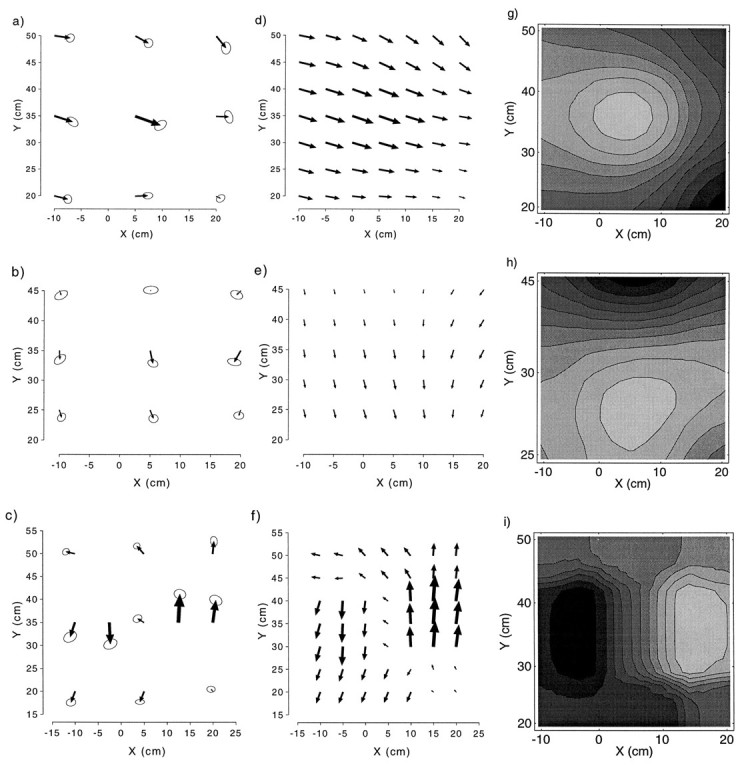
Average change in pointing for the one-pointx-shift (a), one-pointy-shift (b), and two-pointy-shift (c) groups. Smoothed vector field of changes for one-point x-shift (d), one-point y-shift (e), and two-pointy-shift (f) groups. Proportion adaptation relative to the size of the perturbation for the one-point x-shift (g), one-pointy-shift (h), and two-pointy-shift (i) groups. In g, the lightest shade corresponds to 40% adaptation and the darkest shade corresponds to 11% adaptation; inh, the lightest shade corresponds to 16% adaptation and the darkest shade corresponds to 6% adaptation; in i, the lightest shadecorresponds to 58% adaptation in the positive ydirection, and the darkest shade corresponds to 42% adaptation in the negative y direction.

The interpolated vector field of changes for the x-shift group (Fig. 7d) shows a pattern of decaying rightward changes with a downward y trend farther from the subject. The proportion adaptation in the direction of the perturbation computed from the vector fields is depicted in Figure 7g as a gray scale contour plot. This shows that the pattern of greatest change occurs at the training point and decays with distance away from it.

The pattern of generalization for the y-shift group is shown in Figure 7b. The change in pointing between the pre- and postexposure phases was significant at one of nine targets (target 8) in the x direction and at three of nine targets (targets 1, 2, and 5) in the y direction. As in the x-shift group, the shift was again greatest at the training point (2.2 cm). Changes were most pronounced at the two rows closest to the subject; there were no significant changes in the row of targets farthest from the subject. The overall ANOVA indicated that the ydirection of change in the y-shift group was marginally significant (F_(1,7) = 3.75; p = 0.09).

The interpolated vector field of changes for the y-shift group is shown in Figure 7e. This highlights the pattern of downward (i.e., toward the body) changes decaying away from the training point. The proportion adaptation contour plot (Fig.7h) again highlights a pattern of adaptation that is greatest near the training point and decays away from it.

Figure 7c shows the pattern of generalization for the two-point y-shift group. The change in pointing between the pre- and postexposure phases was significant at 2 of 11 targets (targets 3 and 6) in the x direction and at 4 of 11 targets (targets 8–11) in the y direction. Additional marginally significant (p < 0.10) changes occurred at 1 target (target 4) in the x direction and at 4 of 11 targets (targets 1, 2, 4, and 6) in the y direction. The change was greatest at the right training point (6.2 cm), followed by the target immediately to its right (4.9 cm), and then at the left training point (4.7 cm).

The interpolated vector field for the two-point y-shift group (Fig. 7f) shows a change in pointing away from the body in the top right half of the workspace and toward the body in the bottom left half. The ANOVA showed no significant main effects of phase but a highly significant interaction of phase and target in they direction (F_(10,70) = 12.7;p < 0.001), reflecting the nonlinear effect. The corresponding gray scale contour plot shows two areas of adaptation in opposite directions centered around each of the two targets (Fig.7i).

Simulation results

When exposed to each of the three experimental perturbations, the pointing behavior of the model adapts in the compensatory direction. Adaptation is largest at the training point and decays away from it (Fig. 8a–c). The decay is symmetric around the training points in Cartesian coordinates (Fig.8d–f).

Fig. 8.

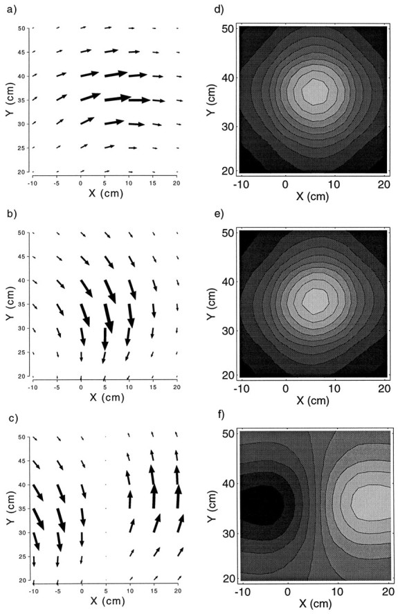
Pattern of generalization for the model under each of the three different experimental conditions. Average change in pointing for the one-point x-shift (a), one-point y-shift (b), and two-pointy-shift (c) conditions. This was computed by subtracting preexposure from postexposure pointing of the model to targets at 5 cm intervals over the workspace. Proportion adaptation relative to the size of the perturbation for the one-pointx-shift (d), one-pointy-shift (e), and two-pointy-shift (f) conditions.

DISCUSSION

Summarizing the results, a remapping of one and two points in the human visuomotor transformation induced changes in pointing at other loci in the workspace. Changes were greatest at the site of the perturbation and decayed away from it. When opposite perturbations were imposed at two points in the visuomotor map, the changes in pointing decayed away from each point. The pattern of generalization resulting from the two-point remapping suggests that the effect of a perturbation at multiple points may be the superposition of the effects at each point.

Referring back to the qualitative models (Fig. 1), the pattern of generalization, although broadly classifiable as nonlinear, closely resembles the Cartesian decaying pattern. Several specific models can be ruled out. First, the pattern of generalization in all three experimental groups was nonlinear, and therefore inconsistent with models in which adaptation is constrained to be linear (Bedford, 1989;Bedford, 1993a). Two factors could account for the discrepancy between our results and Bedford’s. First, Bedford examined adaptation along a constant depth arc, whereas our experiment examined adaptation in the plane. Nonlinear adaptation, when projected onto a lower dimensional subspace, may appear linear. Second, differences in methodology could have contributed to this discrepancy: our experimental setup allowed the finger and visual feedback cursor to be colocated in space, whereas in Bedford’s setup the target feedback was distant from the finger.Bedford (1993b) has subsequently examined adaptation in the horizontal plane using a tablet and monitor setup, and found that certain linear transformations, such as changes in scale, are easier to learn than other transformations. Her results do not, however, address generalization from one point to another in the plane.

Second, the data from the one-point groups are not consistent with a model in which adaptation is represented as a change in felt direction of gaze (Harris, 1965). Because of the arrangement of the chin rest and table, the subjects’ eyes are sagittally away from and above the position of the training point. If adaptation were represented as a constant angular offset in the felt direction of gaze, one would have expected larger shifts in pointing at the more distant targets for both the x- and y-shift groups; in fact, these shifts were generally smaller.

Finally, the opposite-direction perturbations in the two-point remapping condition could have been interpreted by the visuomotor system as a single, counterclockwise rotation around the central target. However, this hypothesis is also not supported by the data, as it predicts large opposite-sign x-shifts at the middle-top and middle-bottom targets, and neither these nor the other peripheral targets demonstrate this rotatory pattern of changes.

Assumptions and limitations of the model

The effects of locally perturbing the visuomotor transformation were qualitatively captured by a simple network model consisting of sensorimotor units with localized Gaussian receptive fields. In this model, the population activity of the units determined the motor command in response to a visual target. Learning took place through pairing the visually and proprioceptively sensed locations of the hand.

The model simplifies the sensorimotor transformation in several ways. Clearly, the visual target location does not arrive in Cartesian body-centered coordinates, but is transformed from retinotopic coordinates using eye position and head orientation information. Neurophysiological data suggest that, at this level of the transformation, neurons in posterior parietal cortex have large retinotopic receptive fields modulated by eye position and head orientation (Andersen, 1987; Snyder et al., 1993). It is still a topic of debate whether this representation is body-centered (Zipser and Andersen, 1988) or some distributed combination of coordinates (Pouget and Sejnowski, 1995). In either case, this representation contains enough information to extract the body-centered coordinates used in our model. The model also simplifies the motor process by coding motor outputs as desired joint angles, rather than modeling the complex dynamic pattern of muscle activation leading the hand to the target.

In the model, the output of the sensorimotor transformation is computed through a population average of the units’ outputs—a feature that was motivated by evidence for population coding in the motor cortex (Georgopoulos et al., 1983, 1986) (see also the closely related model by Salinas and Abbott, 1995). Evidence from the same group suggests that this population activity codes movement vectors in extrinsic (task) coordinates. In the model, we adopt an output representation in joint coordinates, which is more in line with recent results suggesting that movement representation in primary motor cortex is modulated by initial joint coordinates (Scott and Kalaska, 1995).

In the experimental data, the one-point x perturbation induced larger changes in pointing than the one-point yperturbation. This difference was not predicted by the model, which assumes that both the learning rates and receptive field sizes are isotropic. Two factors could account for the anisotropy observed in the human data. First, the visuomotor map may be more adaptable to shifts in the x (transverse) direction, than to shifts in they (combined sagittal and depth) direction. Such a difference in adaptability could be attributable to anisotropies in the geometry and dynamics of the limb and may also explain the somewhat asymmetric pattern of decay. The model could accommodate these differences by using separate learning rates for the two directions, although it may be desirable to account for the dynamics of the limb during movement in a more complex model. Second, the effect could be perceptual; i.e., a less salient perturbation could result in smaller adaptation. In fact, although the magnitude of the perturbations was equal in extrinsic space, the visual angle subtended was smaller for the yperturbation than for the x perturbation.

The function approximation framework

Both the experimental results and the model can be interpreted within the computational framework of function approximation. In this framework, learning the visuomotor transformation consists of approximating the mapping between visual and motor coordinates. Because there are infinitely many possible mappings consistent with any finite set of input–output pairs, the problem is clearly ill-posed. The mathematical theory of function approximation suggests that to obtain a solution to this ill-posed problem, constraints have to be placed on the function approximator (Tikhonov and Arsenin, 1977).

For our experiment, the “function approximator” is the visuomotor system, which is faced with the ill-posed problem of recalibrating its mapping based on one or two novel visuomotor pairings. The pattern of recalibration that results from this limited exposure reflects the structure and constraints underlying the visuomotor map. For example, if the visuomotor map were represented as a look-up table storing corresponding input–output pairs (Atkeson, 1989; Rosenbaum et al., 1993), training at one point would simply change the pairing at that point while leaving unaltered previously learned pairings. At the other extreme, the visuomotor mapping could be represented parametrically, by vectorially combining the retinal location of the target with estimates of eye position and head position to produce body-centered target coordinates. For this system, adaptation constitutes a global recalibration, such as an added bias or scaling, of these estimated sensory inputs (Harris, 1965; Craske, 1967;Lackner, 1973). The pattern of generalization observed in our experiment, therefore, is inconsistent with both local look-up table representations and global parametric representations.

The computational model that captures the data is a form of function approximator intermediate between local and global models known as a radial basis function network (Broomhead and Lowe, 1988;Moody and Darken, 1989). These networks approximate the function via a superposition of bases, in our case the Gaussian receptive fields, and can be derived by assuming that the function approximator trades off the closeness of the fit to the input–output data and the smoothness of the resulting function (Poggio and Girosi, 1989). In other words, such a system is intrinsically biased toward learning smooth mappings.

Other generalization studies

Using a setup in which hand movements produced cursor movements on a monitor, Imamizu et al. (1995) examined pointing under a 75° rotatory perturbation. The results of their study indicate that learning this rotation on movements in one direction generalized to movements in another direction. Subjects were fully informed of the nature and amount of the perturbation; therefore, the experiment confounds perceptual and cognitive components of the task, and the study consequently may bear more on task learning than on the representation of the visuomotor mapping.

Recently, Ghilardi et al. (1995) have examined visuomotor generalization of directional biases. Also using a tablet–monitor setup, they demonstrated that learning to eliminate directional biases in reaching from one initial position produced changes in directional biases from other positions. Both their results and their conclusion—that visuomotor learning is not limited to the area of training—are consistent with ours.

Shadmehr and Mussa-Ivaldi (1994) studied adaptation and generalization to velocity-dependent force fields during target-directed movements. They found that exposure to a force field in the left portion of the workspace generalized to the right portion of the workspace in joint-based, rather than Cartesian, coordinates. There are at least two forms that joint-based generalization could take in the context of our kinematic experiments. First, generalization could be represented as an offset in the perceived joint angles. This is analogous to Shadmehr and Mussa-Ivaldi’s model of dynamic generalization, which was represented as an offset in the external torque. Such generalization would result in a rotatory pattern of changes similar to Figure 1c, with larger changes at the more distal points. Our results were not consistent with this hypothesis. Second, generalization could again be decaying, but the decay may be in joint-based coordinates. Because the Jacobian relating joint angles to Cartesian coordinates is approximately linear in the range of the decay we observed, it is very difficult to distinguish this possibility from Cartesian decaying generalization. However, independent evidence from studies of adaptation to visual distortions of point-to-point movement suggests that the kinematics of arm movement is planned in extrinsic coordinates (Wolpert et al., 1995). These results may indicate an interesting dichotomy between the representation of kinematics, in extrinsic coordinates, and dynamics, in intrinsic joint-based coordinates.

The paradigm of locally perturbing the inputs to the CNS and observing the ensuing pattern of generalization provides us with a unique window into mechanisms of learning and plasticity. By combining this behavioral paradigm with neurophysiological experiments in parietal cortex, it may be possible to determine whether the visuomotor changes are a result of a dynamic reorganization of receptive and motor fields similar to those found in somatosensory and primary motor areas (Donoghue et al., 1990; Sanes et al., 1990; Recanzone et al., 1992). Finally, the decaying pattern of generalization observed may reflect a basic strategy of the CNS whereby computations are distributed over many units with local receptive fields. To test the generality of these findings, it would be interesting to examine the generalization to local remappings in other sensorimotor systems, such as the midbrain tectum, which maintains aligned maps of visual and auditory space (Harris et al., 1980; Knudsen, 1982; Jay and Sparks, 1984; Stein and Meredith, 1993) and is known to adapt to visual displacements (Knudsen and Knudsen, 1989).

REFERENCES

- 1.Andersen RA. Inferior parietal lobule function in spatial perception and visuomotor integration. In: Plum F, Mountcastle V, editors. Handbook of physiology: the nervous system. Higher functions of the brain. American Physiological Society; Rockville, MD: 1987. pp. 483–518. [Google Scholar]
- 2.Andersen RA, Essick C, Siegel R. Encoding of spatial location by posterior parietal neurons. Science. 1985;230:456–458. doi: 10.1126/science.4048942. [DOI] [PubMed] [Google Scholar]
- 3.Atkeson CG. Learning arm kinematics and dynamics. Annu Rev Neurosci. 1989;12:157–183. doi: 10.1146/annurev.ne.12.030189.001105. [DOI] [PubMed] [Google Scholar]
- 4.Bedford F. Constraints on learning new mappings between perceptual dimensions. J Exp Psychol Hum Percept Perform. 1989;15:232–248. [Google Scholar]
- 5.Bedford F. Perceptual and cognitive spatial learning. J Exp Psychol Hum Percept Perform. 1993a;19:517–530. doi: 10.1037//0096-1523.19.3.517. [DOI] [PubMed] [Google Scholar]
- 6.Bedford F. Perceptual learning. In: Medin D, editor. The psychology of learning and motivation, Vol 30. Academic; New York: 1993b. pp. 1–60. [Google Scholar]
- 7.Broomhead DS, Lowe D. Multivariable functional interpolation and adaptive networks. Complex Systems. 1988;2:321–355. [Google Scholar]
- 8.Craske B. Adaptation to prisms: change in internally registered eye-position. Br J Psychol. 1967;58:329–335. doi: 10.1111/j.2044-8295.1967.tb01089.x. [DOI] [PubMed] [Google Scholar]
- 9.Donoghue JP, Suner S, Sanes JN. Dynamic organization of primary motor cortex output to target muscles in adult rats. II. Rapid reorganization following motor or mixed peripheral nerve lesions. Exp Brain Res. 1990;79:492–503. doi: 10.1007/BF00229319. [DOI] [PubMed] [Google Scholar]
- 10.Flanders M, Soechting JF, Tillery SIH. Early stages in a sensorimotor transformation. Behav Brain Sci. 1992;15:309–362. [Google Scholar]
- 11.Georgopoulos AP, Caminiti R, Kalaska JF, Massey JT. Spatial coding of movement: a hypothesis concerning the coding of movement direction by motor cortical populations. Exp Brain Res [Suppl] 1983;7:327–336. [Google Scholar]
- 12.Georgopoulos AP, Schwartz AB, Kettner RE. Neuronal population coding of movement direction. Science. 1986;233:1416–1419. doi: 10.1126/science.3749885. [DOI] [PubMed] [Google Scholar]
- 13.Ghilardi M, Gordon J, Ghez C. Learning a visuomotor transformation in a local area of work space produces directional biases in other areas. J Neurophysiol. 1995;73:2535–2539. doi: 10.1152/jn.1995.73.6.2535. [DOI] [PubMed] [Google Scholar]
- 14.Harris CS. Perceptual adaptation to inverted, reversed, and displaced vision. Psychol Rev. 1965;72:419–444. doi: 10.1037/h0022616. [DOI] [PubMed] [Google Scholar]
- 15.Harris LR, Blakemore C, Donaghy M. Integration of visual and auditory space in the mammalian superior colliculus. Nature. 1980;288:56–59. doi: 10.1038/288056a0. [DOI] [PubMed] [Google Scholar]
- 16.Hay JC, Pick HL. Gaze-contingent prism adaptation: optical and motor factors. J Exp Psychol. 1966;72:640–648. doi: 10.1037/h0023737. [DOI] [PubMed] [Google Scholar]
- 17.Howard IP (1982) Human visual orientation. Chichester, UK: Wiley.
- 18.Imamizu H, Uno Y, Kawato M. Internal representations of the motor apparatus: implications from generalization in visuomotor learning. J Exp Psychol Hum Percept Perform. 1995;21:1174–1198. doi: 10.1037//0096-1523.21.5.1174. [DOI] [PubMed] [Google Scholar]
- 19.Jay MF, Sparks DL. Auditory receptive fields in primate superior colliculus shift with changes in eye position. Nature. 1984;309:345–347. doi: 10.1038/309345a0. [DOI] [PubMed] [Google Scholar]
- 20.Kalaska JF, Crammond DJ. Cerebral cortical mechanisms of reaching movements. Science. 1992;255:1517–1523. doi: 10.1126/science.1549781. [DOI] [PubMed] [Google Scholar]
- 21.Knudsen EI. Auditory and visual maps of space in the optic tectum of the owl. J Neurosci. 1982;2:1177–1194. doi: 10.1523/JNEUROSCI.02-09-01177.1982. [DOI] [PMC free article] [PubMed] [Google Scholar]
- 22.Knudsen EI, Knudsen PF. Vision calibrates sound localization in developing barn owls. J Neurosci. 1989;9:3306–3313. doi: 10.1523/JNEUROSCI.09-09-03306.1989. [DOI] [PMC free article] [PubMed] [Google Scholar]
- 23.Lackner JR. Visual rearrangement affects auditory localization. Neuropsychologia. 1973;11:29–32. doi: 10.1016/0028-3932(73)90061-4. [DOI] [PubMed] [Google Scholar]
- 24.Moody J, Darken C. Fast learning in networks of locally-tuned processing units. Neural Comput. 1989;1:281–294. [Google Scholar]
- 25.Poggio T, Girosi F (1989) A theory of networks for approximation and learning. Artificial Intelligence Lab Memo 1140, MIT.
- 26.Pouget A, Sejnowski T. Spatial representation in the parietal cortex may use basis functions. In: Tesauro G, Touretzky D, Leen T, editors. Advances in neural information processing systems 7. MIT; Cambridge, MA: 1995. pp. 157–164. [Google Scholar]
- 27.Recanzone GH, Merzenich MM, Jenkins WM, Grajski KA, Dinse HR. Topographic reorganization of the hand representation in cortical area 3b of owl monkeys trained on a frequency discrimination task. J Neurophysiol. 1992;67:1031–1056. doi: 10.1152/jn.1992.67.5.1031. [DOI] [PubMed] [Google Scholar]
- 28.Rosenbaum DA, Engelbrecht SE, Bushe MM, Loukopoulos LD. Knowledge model for selecting and producing reaching movements. J Mot Behav. 1993;25:217–227. doi: 10.1080/00222895.1993.9942051. [DOI] [PubMed] [Google Scholar]
- 29.Salinas E, Abbott LF. Transfer of coded information from sensory to motor networks. J Neurosci. 1995;15:6461. doi: 10.1523/JNEUROSCI.15-10-06461.1995. [DOI] [PMC free article] [PubMed] [Google Scholar]
- 30.Sanes JN, Suner S, Donoghue JP. Dynamic organization of primary motor cortex output to target muscles in adult rats. I. Long-term patterns of reorganization following motor or mixed peripheral nerve lesions. Exp Brain Res. 1990;79:479–491. doi: 10.1007/BF00229318. [DOI] [PubMed] [Google Scholar]
- 31.Scott SH, Kalaska JF. Changes in motor cortex activity during reaching movements with similar hand paths but different arm postures. J Neurophysiol. 1995;73:2563–2567. doi: 10.1152/jn.1995.73.6.2563. [DOI] [PubMed] [Google Scholar]
- 32.Shadmehr R, Mussa-Ivaldi F. Adaptive representation of dynamics during learning of a motor task. J Neurosci. 1994;14:3208–3224. doi: 10.1523/JNEUROSCI.14-05-03208.1994. [DOI] [PMC free article] [PubMed] [Google Scholar]
- 33.Snyder LH, Brotchie P, Andersen RA. World-centered encoding of location in posterior parietal cortex of monkey. Soc Neurosci Abstr. 1993;19:770. [Google Scholar]
- 34.Soechting JF, Flanders M. Errors in pointing are due to approximations in sensorimotor transformations. J Neurophysiol. 1989a;62:595–608. doi: 10.1152/jn.1989.62.2.595. [DOI] [PubMed] [Google Scholar]
- 35.Soechting JF, Flanders M. Sensorimotor representations for pointing to targets in three-dimensional space. J Neurophysiol. 1989b;62:582–594. doi: 10.1152/jn.1989.62.2.582. [DOI] [PubMed] [Google Scholar]
- 36.Stein BE, Meredith MA (1993) The merging of the senses. Cambridge, MA: MIT.
- 37.Stratton GM. Upright vision and the retinal image. Psychol Rev. 1897a;4:182–187. [Google Scholar]
- 38.Stratton GM (1897b) Vision without inversion of the retinal image. Psychol Rev 4:341–360, 463–481.
- 39.Tikhonov AN, Arsenin VY (1977) Solutions of ill-posed problems. Washington, D.C.: W. H. Winston.
- 40.von Helmholtz H (1867) Treatise on physiological optics. Rochester, NY: Optical Society of America.
- 41.Welch RB (1978) Perceptual modification. New York: Academic.
- 42. Welch RB. Adaptation to space perception. Boff K, Kaufman L, Thomas J. Handbook of perception and performance, Vol 1 1986. 24.1 24.45 Wiley; New York-Interscience. [Google Scholar]
- 43.Wolpert DM, Ghahramani Z, Jordan MI. Are arm trajectories planned in kinematic or dynamic coordinates? An adaptation study. Exp Brain Res. 1995;103:460–470. doi: 10.1007/BF00241505. [DOI] [PubMed] [Google Scholar]
- 44.Zipser D, Andersen RA. A back-propagation programmed network that simulates response properties of a subset of posterior parietal neurons. Nature. 1988;331:679–684. doi: 10.1038/331679a0. [DOI] [PubMed] [Google Scholar]