Bayesian factorizations of big sparse tensors

Abstract

It has become routine to collect data that are structured as multiway arrays (tensors). There is an enormous literature on low rank and sparse matrix factorizations, but limited consideration of extensions to the tensor case in statistics. The most common low rank tensor factorization relies on parallel factor analysis (PARAFAC), which expresses a rank k tensor as a sum of rank one tensors. When observations are only available for a tiny subset of the cells of a big tensor, the low rank assumption is not sufficient and PARAFAC has poor performance. We induce an additional layer of dimension reduction by allowing the effective rank to vary across dimensions of the table. For concreteness, we focus on a contingency table application. Taking a Bayesian approach, we place priors on terms in the factorization and develop an efficient Gibbs sampler for posterior computation. Theory is provided showing posterior concentration rates in high-dimensional settings, and the methods are shown to have excellent performance in simulations and several real data applications.

1. Introduction

Sparsely observed big tabular data sets are commonly collected in many applied domains. One example corresponds to recommender systems in which the dimensions of the table correspond to users, items and different contexts (Karatzoglou et al. (2010)), with a tiny proportion of the cells filled in for users providing rankings. The task is to fill in the rest of the huge table in order to make recommendations to users of which items they may prefer in each context. This extends the widely studied matrix completion problem (Candes and Recht (2009)) of which the Netflix challenge was one example. Another setting corresponds to contingency tables in which multivariate categorical data are collected for each individual, and the cells of the table contain counts of the number of individuals having a particular combination of values. In contingency table analyses, the focus is typically on inferring associations among the different variables, but challenges arise when there are many variables, so that the number of cells in the table is vastly bigger than the sample size.

Suppose that the tensor of interest is $\pi \in {\prod }_{d_1\times \cdots \times d_p}$, with ${\prod }_{d_1\times \cdots \times d_p}$ a space of p-way tensors having d_j rows in the jth direction. Often there are constraints on the elements of the tensor. For recommender systems, ratings are non-negative so that one is faced with a non-negative tensor factorization problem (Paatero and Tapper (1994); Lee and Seung (1999); Friedlander and Hatz (2005); Lim and Comon (2009); Liu et al. (2012)). For contingency tables, the tensor corresponds to the joint probability mass function for multivariate categorical data, so that the elements are non-negative and add to one across all the cells (Dunson and Xing (2009); Bhattacharya and Dunson (2012)). Let Y denote the data collected on tensor π. For recommender systems, Y consists of ratings for a small subset of the ${\prod }_{j=1}^p{d}_j$ cells in the tensor, while for contingency tables Y includes response vectors y_i = (y_i1,…, y_ip)^T for subjects i = 1, …, n, with y_ij ∈ {1, …, d_j} for j = 1, …, p. In both cases, data are extremely sparse, with no observations in the overwhelming majority of cells.

To combat this data sparsity, it is necessary to substantially reduce dimensionality in estimating π. The usual way to accomplish this is through a low rank assumption. Unlike for matrices, there is no unique definition of rank but the most common convention is to define the rank k of a tensor π as the smallest value of k such that π can be expressed as

$$\pi =\sum _{h=1}^k{\psi }_h^{(1)}\otimes \cdots \otimes {\psi }_h^{(p)},$$ (1)

which is sum of k rank one tensors, each an outer product of vectors¹ for each dimension (Kolda and Bader, 2009). Expression (1) is commonly referred to as parallel factor analysis (PARAFAC) (Harshman (1970); Bro (1997)). For k small, the number of parameters is massively reduced from ${\prod }_{j=1}^p{d}_j$ to $k{\sum }_{j=1}^p{d}_j$; as the low rank assumption often holds approximately, this leads to an effective approach in many applications, and a rich variety of algorithms are available for estimation.

However, the decrease in degrees of freedom from exponential in p to linear in p is not sufficient when p is big. Large p small n problems arise routinely, and a usual solution outside of tensor settings is to incorporate sparsity. For example, in linear regression, many of the coefficients are set to zero, while in estimation of large covariance matrices, sparse factor models are used that assume few factors and many zeros in the factor loadings matrices (West (2003); Carvalho et al. (2008)). In the matrix factorization literature, there has been consideration of low rank plus sparse decompositions (Chartrand (2012)), but this approach does not solve our problem of too many parameters. Including zeros in the component vectors $\left\{{\psi }_h^{(j)}\right\}$ is not a viable solution, particularly as we do not want to enforce exact zeros in blocks of the tensor π but require an alternative notion of sparsity.

Our notion is as follows. For component h (h = 1, …, k), we partition the dimensions into two mutually exclusive subsets $S_h\cup S_h^c=\{1,\dots ,p\}$. The proposed sparse PARAFAC (sp-PARAFAC) factorization is then

$$\pi =\sum _{h=1}^k{\psi }_h^{(1)}\otimes \cdots \otimes {\psi }_h^{(p)},{\psi }_h^{(j)}={\psi }_0^{(j)}\text{ for }j\in S_h^c.$$ (2)

Hence, instead of having to introduce a separate vector ${\psi }_h^{(j)}$ for every h and j, we allow there to be more degrees of freedom used to characterize the tensor structure in certain directions than in others. Consider the recommender systems application and suppose we have three dimensions, including users (j = 1), items (j = 2) and context (j = 3). If we let ${\psi }_h^{(3)}={\psi }_0^{(3)}$ for h = 1, …, k,

$${\pi }_{c_1{c}_2{c}_3}={\psi }_{0c_3}^{(3)}\sum _{h=1}^k{\psi }_{h{c}_1}^{(1)}{\psi }_{h{c}_2}^{(2)},$$ (3)

so that we factorize the user-item matrix as being of rank k, and then include a multiplier specific to each level of the context factor. This assumes that users rank systematically higher or lower depending on context but there is no interaction. In the contingency table application, $\text{Pr} (y_{i1}=c_1,\dots ,y_{ip}=c_p)={\pi }_{c_1\cdots c_p}$. If $j\in S_h^c$ for h = 1, …, k, then the jth variable is independent of the other variables with $\text{Pr} \left(y_{ij}=c_j\right)={\psi }_{0c_j}^{(j)}$. By including $j\in S_h^c$ for some but not all h ∈ {1, …, k} one can use fewer degrees of freedom in characterizing the interaction between the jth factor and the other factors. In practice, we will learn {S_h} using a Bayesian approach, as the appropriate lower dimensional structure is typically not known in advance.

We conjecture that many tensor data sets can be concisely represented via (2), with results substantially improved over usual PARAFAC factorizations due to the second layer of dimension reduction. For concreteness and brevity, we focus on contingency tables, but the methods are easily modified to other settings. Contingency table analysis is routine in practice; refer to Agresti (2002); Fienberg and Rinaldo (2007). However, in stark contrast to the well developed literature on linear regression and covariance matrix estimation in big data settings, very few flexible methods are scalable beyond small tables. Throughout the rest of the paper, we assume that the observed data y_i = (y_i1, …, y_ip)^T, i = 1, …, n, is multivariate unordered categorical, with y_ij· ∈ {1, …, d_j}. Our interest is in situations where the dimensionality p is comparable or even larger than the number of samples n.

2. Sparse Factor Models for Tables

2.1. Model and prior

We focus on a Bayesian implementation of sp-PARAFAC in (2). Let ${\mathcal{S}}^{r-1}=\left\{x\in {\Re }^r:x_j\ge 0,{\sum }_{j=1}^r{x}_j=1\right\}$ denote the (r − 1)-dimensional probability simplex. In the contingency table case, Dunson and Xing (2009) proposed the following probabilistic PARAFAC factorization.

$$\text{Pr }\left(y_{i1}=c_1,\dots ,y_{ip}=c_p\right)={\pi }_{c_1\cdots c_p}=\sum _{h=1}^k{\nu }_h\prod _{j=1}^p{\lambda }_{h{c}_j}^{(j)},$$ (4)

where $\nu =\left\{{\nu }_h\right\}\in {\mathcal{S}}^{k-1}$ and ${\lambda }_h^{(j)}=\left({\lambda }_{h1}^{(j)},\dots ,{\lambda }_{h{d}_j}^{(j)}\right)\in {\mathcal{S}}^{d_j-1}$ is a vector of probabilities of y_ij = 1, …, d_j in component h. Introducing a latent sub-population index z_i ∈ {1, …, k} for subject i, the elements of y_i are conditionally independent given z_i with $\text{Pr }\left(y_{ij}=c_j|z_i=h\right)={\lambda }_{h{c}_j}^{(j)}$, and marginalizing out the latent index z_i leads to a mixture of product multinomial distribution for y_i. Placing Dirichlet priors on the component vectors leads to a simple and efficient Gibbs sampler for posterior computation. We will refer to this model (4) as standard PARAFAC.

This approach has excellent performance in small to moderate p problems, but as p increases there is an inevitable breakdown point. The number of parameters increases linearly in p, as for other PARAFAC factorizations, so problems arise as p approaches the order of n or p ≫ n. For example, we are particularly motivated by epidemiology studies collecting many categorical predictors, such as occupation type, demographic variables, and single nucleotide polymorphisms. For continuous response vectors $y_i\in {\Re }^p$, there is a well developed literature on Gaussian sparse factor models that are adept at accommodating p ≫ n data (West (2003); Lucas et al. (2006); Carvalho et al. (2008); Bhattacharya and Dunson (2011)). These models include many zeros in the loadings matrices to induce additional dimension reduction on top of the low rank assumption. Pati et al. (2013a) provided theoretical support through characterizing posterior concentration.

Our sp-PARAFAC factorization provides an analog of sparse factor models in the tensor setting. Modifying for the categorical data case, we let

$${\pi }_{c_1\dots c_p}=\sum _{h=1}^k{\nu }_h\prod _{j\in S_h}{\lambda }_{h{c}_j}^{(j)}\prod _{j\in S_h^c}{\lambda }_{0c_j}^{(j)},$$ (5)

where |S_h| ≪ p(|S| denotes the cardinality of a set S) and the ${\lambda }_0^{(j)}$ vectors are fixed in advance; we consider two cases:

$$(i){\lambda }_0^{(j)}={\left(\frac{1}{d_j},\dots ,\frac{1}{d_j}\right)}^{\text{T}}\text{ and }(ii){\lambda }_0^{(j)}={\left(\frac{1}{n}\sum _{i=1}^n{y}_{i1},\dots ,\frac{1}{n}\sum _{i=1}^n{y}_{ip}\right)}^{\text{T}},$$

corresponding to a discrete uniform and empirical estimates of the marginal category probabilities. By fixing the baseline dictionary vectors $\left\{{\lambda }_0^{(j)}\right\}$ in advance, and allocating a large subset of the variables within each cluster h to the baseline component, we dramatically reduce the size of the model space. In particular, the probability tensor π in (5) can be parameterized as ${\theta }_{\pi }=\left(\nu ,{\left\{S_h\right\}}_{1\le h\le k},{\left\{{\lambda }_h^{(j)}\right\}}_{1\le h\le k,j\in S_h}\right)$, where $\nu \in {\mathcal{S}}^{k-1},S_h\subset \{1,\dots ,p\},{\lambda }_h^{(j)}\in {\mathcal{S}}^{d_j-1}$. Thus, the effective number of model parameters is now reduced to $(k-1)+{\sum }_{h=1}^k\left|S_h\right|+{\sum }_{h=1}^k{\sum }_{j\in S_h}\left(d_j-1\right)$, which is substantially smaller than the $(k-1)+{\sum }_{j=1}^{p}k\left(d_j-1\right)$ parameters in the original specification, provided |S_h| ≪ p for all h = 1, … k. This is ensured via a sparsity favoring prior on |S_h| below. We will illustrate that this can lead to huge differences in practical performance.

Completing a Bayesian specification with priors for the unknown parameter vectors and expressing the model in hierarchical form, we have²

$$\begin{gathered} y_{ij}~\text{ Mult }\left(\left\{1,\dots ,d_j\right\};{\lambda }_{z_{1}1}^{(j)},\dots ,{\lambda }_{z_i{d}_j}^{(j)}\right), \\ {\lambda }_h^{(j)}~\left(1-{\tau }_h\right){\delta }_{{\lambda }_0^{(j)}}+{\tau }_h\text{ Diri }\left(a_{j1},\dots ,a_{j{d}_j}\right), \\ \text{ Pr}\left(z_i=h\right)={\nu }_h=V_h{\prod }_{l<h}\left(1-V_l\right), \\ {V}_h~\text{ Beta }(1,\alpha ),\alpha ~\text{ Gamma }\left(a_{\alpha },b_{\alpha }\right),{\tau }_h~\text{ Beta}(1,\gamma ). \end{gathered}$$ (6)

It is evident that the hierarchical prior in (6) is supported on the space of probability tensors with a sp-PARAFAC decomposition as in (5), since (6) is equivalent to letting the subset-size |S_h| ~ Binom(p, τ_h) and drawing a random subset S_h uniformly from all subsets of {1, …, p} of size |S_h| in (5). A stick-breaking prior (Sethuraman, 1994) is chosen for the component weights {ν_h}, taking a nonparametric Bayes approach that allows k = ∞, with a hyperprior placed on the concentration parameter α in the stick-breaking process to allow the data to inform more strongly about the component weights. The probability of allocation τ_h to the active (non-baseline) category in component h is chosen as beta(1, γ), with γ > 1 favoring allocation of many of the ${\lambda }_h^{(j)}$s to the baseline category ${\lambda }_0^{(j)}$. In the limiting case as γ > ∞, the joint probability tensor π becomes an outer product of the baseline probabilities for the individual variables, $\pi ={\lambda }_0^{(1)}\otimes \cdots \otimes {\lambda }_0^{(p)}$. On the other hand, as γ → 0, one reduces back to standard PARAFAC (4).

Line 2 of expression (6) is key in inducing the second level of dimensionality reduction in our Bayesian sparse PARAFAC factorization. The inclusion of the baseline component that does not vary with h massively reduces the number of parameters, and can additionally be argued to have minimal impact on the flexibility of the specification. The ${\lambda }_h^{(j)}$s are incorporated within ${\prod }_{j=1}^p{\lambda }_{h{c}_j}^{(j)}$, which for large p is highly concentrated around its mean since the ${\lambda }_h^{(j)}$‘s are independent across j. This is a manifestation of the concentration of measure phenomenon (Talagrand, 1996), which roughly states that a random variable that depends in a smooth way on the influence of many independent variables, but not too much on any one of them, is essentially constant. For example, if ${\theta }_j\stackrel{iid}{~}U(0,1)$ and $\Theta ={\prod }_{j=1}^p{\theta }_j$, then E(Θ) = (1/2)^p and var(Θ) = (1/3)^p, which rapidly converges to zero. This implies that replacing a large randomly chosen subset of the ${\lambda }_h^{(j)}$s by ${\lambda }_0^{(j)}$ should have minimal impact on modeling flexibility.

2.2. Induced prior in log-linear parameterization

An important challenge is accommodating higher order interactions, which play an important rolein many applications (e.g., genetics), but are typically assumed to equal zero for tractability. As p grows, it is challenging to even accommodate two-way interactions in traditional categorical data models (log-linear, logistic regression) due to an explosion in the number of terms. In contrast, the tensor factorization does not explicitly parameterize interactions, but indirectly induces a shrinkage prior on the terms in a saturated log-linear model. One can then reparameterize in terms of the log-linear model in conducting inferences in a post model-fitting step. We illustrate the induced priors on the main effects and interactions below.

For ease of exposition, we first focus on a case where p = 3 and d_j = d = 2 for j = 1, …, 3. We generate 10, 000 random probability tensors ${\pi }^{(t)}=\left({\pi }_{c_1{c}_2{c}_3}^{(t)}\right)$, t = 1, …, 10, 000 distributed according to (6), where we fix the baseline ${\lambda }_0^{(j)}=(1/2,1/2)$ for all j. Given a 2 × 2 × 2 tensor π, we can equivalently characterize π in terms of its log-linear parameterization

$$\beta ={\left({\beta }_1,{\beta }_2,{\beta }_3,{\beta }_{12},{\beta }_{13},{\beta }_{23},{\beta }_{123}\right)}^{\text{T}},$$

consisting of 3 main effect terms β₁, β₂, β₃, three second-order interaction terms β₁₂, β₁₃, β₂₃ and one third order interaction term β₁₂₃; refer to §5.3.5 of Agresti (2002). Given each prior sample π^(t), we equivalently obtain a sample β^(t) from the induced prior on β, which allows us to estimate the marginal densities of the main effects and interactions and also their joint distributions. In particular, since γ plays an important role in placing weights on the baseline component, we would like to see how our induced priors differ with different γ values.

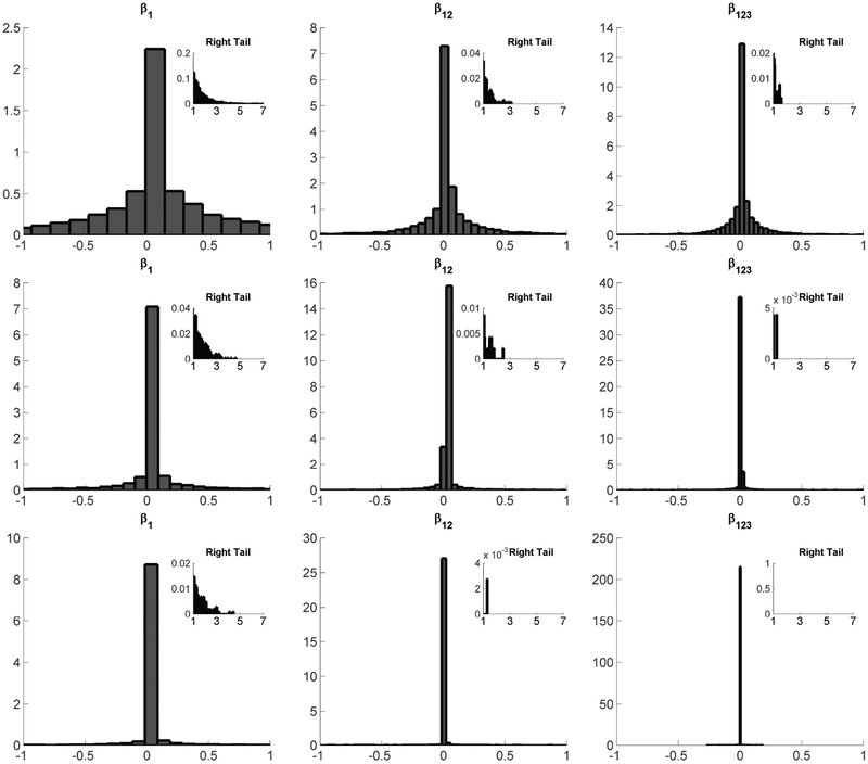
In our simulation exercise, we fix three values of γ, namely, γ = 1, 5, 20. Note that γ = 1 corresponds to a U(0,1) prior on τ_h. For different values of γ, we show the histograms of one main effect term β₁, one two-way interaction β₁₂ and the three-way interaction β₁₂₃ in Figure 1. Table 1 additionally reports summary statistics.

Figure 1:

Histograms of induced priors for one main effect β₁, one two-way interaction β₁₂, and the three-way interaction β₁₂₃ - Top Row: γ = 1; Middle Row: γ = 5; Bottom Row: γ = 20.

Table 1:

Summary statistics of induced priors on coefficients in log-linear model parameterization.

γ	Coefficient	Mean	Std.dev	Min	Max	Skewness	Kurtosis
1	β1	0.014	0.831	−6.765	6.389	0.210	9.109
1	β12	−0.002	0.340	−2.895	3.105	−0.025	16.583
1	β123	0.002	0.196	−2.223	2.632	0.525	24.686
5	β1	−0.002	0.485	−5.648	5.433	0.031	27.980
5	β12	0.000	0.124	−2.085	2.244	0.495	93.438
5	β123	0.000	0.051	−1.214	0.745	−3.701	159.360
20	β1	0.002	0.246	−3.109	5.669	2.474	99.554
20	β12	0.000	0.042	−1.126	1.819	9.488	632.790
20	β123	0.000	0.009	−0.664	0.214	−44.051	3014.000

In high-dimensional regression, $y_i=x_i^{\text{T}}\beta +{ϵ}_i$, there has been substantial interest in shrinkage priors, which draw β_j a priori from a density concentrated at zero with heavy tails. Such priors strongly shrink the small coefficients to zero, while limiting shrinkage of the larger signals (Park and Casella, 2008; Carvalho et al., 2010; Polson and Scott, 2010; Hans, 2011; Armagan et al., 2013a). In Figure 1, the induced prior on any of the log-linear model parameters is symmetric about zero, with a large spike very close to zero, and heavy tails. Thus, we have indirectly induced a continuous shrinkage prior on the main effects and interactions through our tensor decomposition approach. In addition, the prior automatically shrinks more aggressively as the interaction order increases. Such greater shrinkage of interactions is commonly recommended (Gelman et al., 2008). Importantly, we do not zero out small interactions but allow many small coefficients, which is an important distinction in applications, such as genomics, having many small signals. The hyperparameter γ serves as a penalty controlling the degree of shrinkage.

Our next set of simulations involve larger values of p, where the necessity of the regularization implied by γ becomes strikingly evident. In the log-linear parameterization, we now have p main effects β₁, …, β_p; let β_main = (β₁, …, β_p)^T. In the p ≫ n setting, one cannot even hope to consistently recover all the main effects unless a large fraction of the β_j’s are zero or close to zero. One would thus favor a shrinkage prior on β_main, with any particular draw resembling a near-sparse vector. Since the induced prior on the β_j’s is continuous, we study the l₁ norm ${\Vert {\beta }_{main}\Vert }_1={\sum }_{j=1}^p\left|{\beta }_j\right|$ as a surrogate for the l₀ norm to quantify the sparsity.

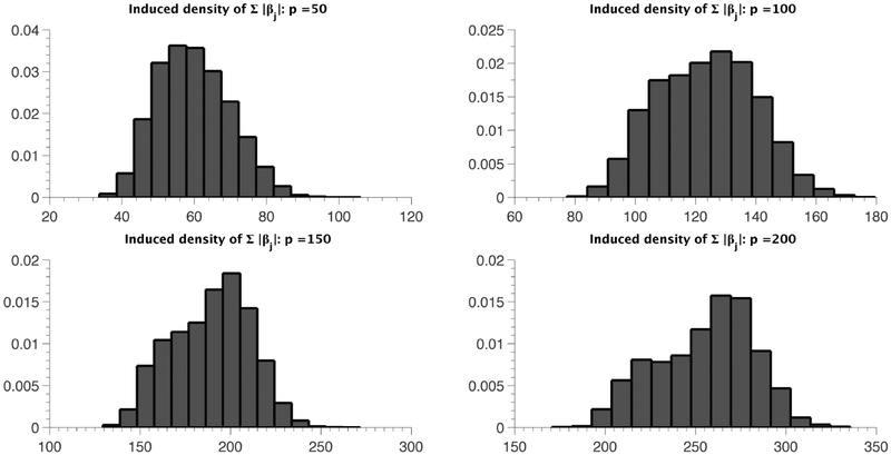
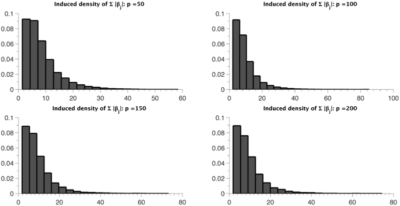
We consider p = 50, 100, 150, 200 and plot histograms of the induced density of ∥β_main∥₁ based on 10, 000 prior draws in Figures 2 and 3. Figure 2 corresponds to the case where γ = 0, i.e., when the sp-PARAFAC formulation reduces back to the standard PARAFAC (4), while γ/p is set to a constant β ∈ (0,1) in Figure 3. Figure 2 reveals a highly undesirable property of the standard PARAFAC in high dimensions, where the entire distribution of ∥β_main∥₁ shifts to the right with increasing p, with $\mathbb{E}{\Vert {\beta }_{main}\Vert }_1\asymp p$. The induced prior clearly lacks any automatic multiplicity adjustment property (Scott and Berger, 2010), and would bias inferences for moderate to large values of p. On the other hand, under the sp-PARAFAC model, the induced prior on ∥β_main∥₁ is robust to increasing p, as evident from Figure 3. The choice γ = βp essentially forces a constant proportion of the variablesto be assigned to the null group; see Castillo and van der Vaart (2012) for a similar choice of the hyper-parameter in a regression setting.3.1 Preliminaries

Figure 2:

Histograms of ∥β_main∥₁ for different values of p under the standard PARAFAC model.

Figure 3:

Histograms of ∥β_main∥₁ for different values of p under the sp-PARAFAC model with γ = 0.1p.

3. Posterior concentration

3.1. Preliminaries

In this section, we provide theoretical justification to the proposed sp-PARAFAC procedure in high dimensional settings by studying the concentration properties of the posterior with growing sample size. When the parameter space is finite dimensional, it is well known that the posterior contracts at the parametric rate of n^−1/2 under mild regularity conditions (Ghosal et al., 2000). However, we are interested in the asymptotic framework of the dimension p = p_n growing with the sample size n, potentially at a faster rate, reflecting the applications we are interested in. There is a small but increasing literature on asymptotic properties of Bayesian procedures in models with growing dimensionality, with most of the focus being on linear models or generalized linear models belonging to the exponential family; refer to Ghosal (1999, 2000); Belitser and Ghosal (2003); Jiang (2007); Armagan et al. (2013b); Bontemps (2011); Castillo and van der Vaart (2012); Yang and Dunson (2013) among others. In all these cases, the object of interest is a vector of high-dimensional regression coefficients or more generally, the conditional distribution f (y | x) of a univariate response y given high-dimensional predictors x. However, our object of interest is significantly different as we are concerned with estimation of the high-dimensional joint probability tensor π.

Let ${\mathcal{F}}_n$ denote the class of all $d_1\times \dots \times d_{p_n}$ probability tensors; we shall assume $d_1=\dots =d_{p_n}=d$ in the sequel for notational convenience. Let ${\pi }^{(0n)}\subset {\mathcal{F}}_n$ be a sequence of true tensors. We observe y₁, …, y_n ~ π⁽⁰ⁿ⁾ and set y⁽ⁿ⁾ = (y₁, …, y_n). We denote the prior distribution on ${\mathcal{F}}_n$ induced by the sp-PARAFAC formulation by ${\mathbb{P}}_n$ and the corresponding posterior distribution by ${\mathbb{P}}_n\left(\cdot |y^{(n)}\right)$.

For two probability tensors π⁽¹⁾ and ${\pi }^{(2)}\in {\mathcal{F}}_n$, the L₁ distance is defined as:

$${\Vert {\pi }^{(1)}-{\pi }^{(2)}\Vert }_1=\sum _{c_1=1}^d\dots \sum _{c_{p_n}=1}^d\left|{\pi }_{c_1\dots c_{p_n}}^{(1)}-{\pi }_{c_1\dots c_{p_n}}^{(2)}\right|.$$

For a sequence of numbers ϵ_n → 0 and a constant M > 0 independent of ϵ_n, let

$$U_n=\left\{\pi :{\Vert \pi -{\pi }^{(0n)}\Vert }_1\le M{ϵ}_n\right\}$$ (7)

denote a ball of radius Mϵ_n around π⁽⁰ⁿ⁾ in the L₁ norm. We seek to find a minimum possible sequence ϵ_n such that

$$\underset{n\to \infty }{\text{lim}}{\mathbb{P}}_n\left(U_n^c|y^{(n)}\right)\to 0,\text{ a.s. }{\pi }^{(0n)}.$$ (8)

3.2. Assumptions

In this section we state our assumptions on the true data generating model and briefly discuss their implications.

Assumption 3.1. The true sequence of probability tensors π⁽⁰ⁿ⁾ are of the form

$${\pi }_{c_1\dots c_{p_n}}^{(0)}=\sum _{h=1}^{k_n}{\nu }_{0h}\prod _{j\in S_{0h}}{\lambda }_{h{c}_j}^{(0j)}\prod _{j\in S_{0h}^c}{\lambda }_{0c_j}^{(j)},1\le c_j\le d,1\le j\le p_n,$$ (A0)

where ${\lambda }_0^{(j)}\in {\mathcal{S}}^{d-1}$ are assumed to be known. Unless otherwise specified, we shall assume ${\lambda }_0^{(j)}=(1/d,\dots ,1/d)$ is the probability vector corresponding to the uniform distribution on {1, …, d}.

We now provide some intuition for assumption (A0). Letting $S_0={\cup }_{h=1}^{k_n}{S}_{0h}$, we can rewrite the expansion of π⁽⁰ⁿ⁾ in (A0) as

$${\pi }_{c_1\dots c_{p_n}}^{(0n)}=\sum _{h=1}^{k_n}{\nu }_{0h}\prod _{j\in S_0}{\overline{\lambda }}_{h{c}_j}^{(0j)}\prod _{j\in S_0^c}{\lambda }_{0c_j}^{(j)},$$ (9)

where

$${\overline{\lambda }}_h^{(0j)}=\{\begin{array}{ll}{\lambda }_h^{(0j)}\hfill & \text{if }j\in S_{0h},\hfill \\ {\lambda }_0^{(j)}\hfill & \text{if }j\in S_0\backslash S_{0h}.\hfill \end{array}$$

In (9), the term ${\prod }_{j\in S_0^c}{\lambda }_{0c_j}^{(j)}$ doesn’t involve h and can be factored out completely. Assumption (A0) thus posits that the variables in $S_0^c$ are marginally independent and the entire dependence structure is driven by the variables in S₀. We shall refer to S₀ and $S_0^c$ as the non-null and null group of variables respectively.

Let q_n = |S₀| and define a mapping j → e_j from {1, …, q_n} to the ordered elements of S₀, so that $e_1\le \dots e_{q_n}$. As j varies between 1 to q_n, e_j ranges over the elements of S₀. Denote by ψ⁽⁰ⁿ⁾ the $d^{q_n}$ joint probability tensor for the variables {y_ij : j ∈ S₀}, so that

$${\psi }_{c_1\dots c_n}^{(0n)}= \text{Pr} \left(y_{i{e}_1}=c_1,\dots ,y_{i{e}_n}=c_n\right)=\sum _{h=1}^{k_n}{\nu }_{0h}\prod _{j=1}^{q_n}{\overline{\lambda }}_{h{c}_j}^{\left(0e_j\right)}.$$ (10)

Thus, after factoring out the marginally independent variables in $S_0^c$, (A0) implies a standard PARAFAC expansion (10) for ψ⁽⁰ⁿ⁾ with k_n many components. Since any non-negative tensor admits a standard PARAFAC distribution (Lim and Comon, 2009), we can always write an expansion of ψ⁽⁰ⁿ⁾ as in (10).

The next set of assumptions are provided below.³

Assumption 3.2. In addition to (A0), π⁽⁰ⁿ⁾ satisfies

(A1) The number of components k_n = O(1).

(A2) Letting $s_n={\text{max}}_{1\le h\le k_n}\left|S_{0h}\right|$, one has s_n = o(log p_n).

(A3) There exists a constant ε_ο ∈ (0,1) such that ${\lambda }_{hc}^{(0j)}\ge {\epsilon }_0$ for all 1 ≤ h ≤ k_n, 1 ≤ c ≤ d, j ∈ S_0h.

(A1) and (A2) imply that the size of the non-null group is much smaller than p_n, since $q_n=\left|S_0\right|\le {\sum }_{h=1}^{k_n}\left|S_h\right|\le k_n{s}_n\ll p_n$.

Some discussion is in order for condition (A3). First, note that we can choose ε₀ in a way so that ${\overline{\lambda }}_{hc}^{(0j)}\ge {\epsilon }_0$ for all h, c and j ∈ S₀. Hence, (A3) implies a lower bound on the joint probability ψ⁽⁰ⁿ⁾ in (10). Such a lower bound on a compactly supported target density is a standard assumption in Bayesian non-parametric theory; see for example van der Vaart and van Zanten (2008). However, unlike univariate or multivariate density estimation in fixed dimensions where the density can be assumed to be bounded below by a constant, we need to precisely characterize the decay rate of the lower bound of the joint probability. Since ψ⁽⁰ⁿ⁾ is a $d^{q_n}$ probability tensor, ${\text{min}}_{c_1,\dots c_{sn}}{\psi }_{c_1\dots c_{s_n}}^{(0n)}\le {(1/d)}^{q_n}=\text{exp}\left(-s_n{k}_n\text{\hspace{0.17em}log\hspace{0.17em}}d\right)$. Assumption (A3) implies that

$$\underset{{}_{c_1,\dots ,c_{sn}}}{\text{min}}{\psi }_{c_1\dots c_{sn}}^{(0n)}\ge \text{exp}\left(-q_n\text{log}\left(1/{\epsilon }_0\right)\right)=\text{exp}\left(-c_0{s}_n\right)$$ (11)

for some constant c₀ > 0.

3.3. Main result

We are now in a position to state a theorem on posterior convergence rates.

Theorem 3.1. Assume the true sequence of tensors ${\pi }^{(0n)}\in {\mathcal{F}}_n$ satisfy assumptions (A0) – (A3) and s_n log p_n/n → 0. Also, assume the sp-PARAFAC model is fitted with the stick-breaking prior truncated to k_n many components and $\gamma =\beta p_n^2$ for some constant β ∈ (0,1) in (6). Then, (8) is satisfied with ${ϵ}_n=\sqrt{s_n\text{\hspace{0.17em}log\hspace{0.17em}}{p}_n/n}$ in (7).

A proof of Theorem 3.1 can be found in the appendix. As an implication of Theorem 3.1, if p_n = n^d for some constant d, then the posterior contracts at the near parametric rate $\sqrt{{(\text{log\hspace{0.17em}}n)}^c/n}$ for some constant c > 0. Moreover, consistent estimation is possible even if p_n is exponentially large as long as $p_n\le \text{exp}(\sqrt{n})$. In particular, with p_n = exp(n^δ/2) for δ < 1, the posterior contracts at least at the rate n^{−(1−δ)/2}.

Remark 3.2. We assume the number of components k_n known in Theorem 3.1 for ease of exposition, with our main focus on dimensionality reduction. Adapting to an unknown number of components in mixture models is a well -studied problem; see, for example, Ge and Jiang (2006); Pati et al. (2013b); Shen et al. (2011). For the infinite stick-breaking prior on the mixture components, one can use the sieving technique developed in Pati et al. (2013b) to estimate deviation bounds for the tail sum of a stick-breaking process.

Remark 3.3. In practice, we recommend the choice γ = βp_n for numerical stability, with β = 0.2 used as a default choice in all our examples. The probability mass function of the induced beta-bernoulli prior on |S_h| with $\gamma =\beta p_n^2$ behaves like exp(−cs log p_n) for small s, while the same is exp(−cs) for γ = βp_n; refer to the proof of Theorem 3.1 for further details.

4. Posterior Computation

Under model (6), we can easily proceed to draw posterior samples from a Gibbs sampler since all the full conditionals have recognizable forms. The algorithm iterates through the following steps:

1. For each j^th variable and latent class h, update ${\lambda }_h^{(j)}\equiv \left({\lambda }_{h1}^{(j)},\dots ,{\lambda }_{h{d}_j}^{(j)}\right)$ from a mixture of two distributions with different weights. Given the prior we specified for ${\lambda }_h^{(j)}$ in (6), the posterior maintains its conjugacy and comes from either a Dirichlet or the baseline category. i.e., for j = 1, …, p, h = 1, …, k*, where k* = max{z₁, …, z_n}:

   $$\left({\lambda }_h^{(j)}|-\right)=w_{0h}^{(j)}{\delta }_{{\lambda }_0^{(j)}}+w_{1h}^{(j)} \text{Diri}\left(a_{j1}+\sum _{i=1}^{n}1\left(y_{ij}=1,z_i=h\right),\dots ,a_{j{d}_j}+\sum _{i=1}^{n}1\left(y_{ij}=d_j,z_i=h\right)\right),$$ (12)

   where $w_{0h}^{(j)}$ and $w_{1h}^{(j)}$ are the mixture weights:

   $$w_{0h}^{(j)}=\frac{\left(1-{\tau }_h\right){\prod }_{c=1}^{d_j}{\lambda }_{0c}^{(j){\sum }_{i=1}^{n}1\left(z_i=h,y_{ij}=c\right)}}{\left(1-{\tau }_h\right){\prod }_{c=1}^{d_j}{\lambda }_{0c}^{(j){\sum }_{i=1}^{n}1\left(z_i=h,y_{ij}=c\right)}+{\tau }_h\frac{\Gamma \left({\sum }_{c=1}^{d_j}{a}_{jc}\right)}{{\prod }_{c=1}^{d_j}\Gamma \left(a_{jc}\right)}\cdot \frac{{\prod }_{c=1}^{d_j}\Gamma \left(a_{jc}+{\sum }_{i=1}^{n}1\left(z_i=h,y_{ij}=c\right)\right)}{\Gamma \left({\sum }_{c=1}^d{a}_{jc}+{\sum }_{i=1}^{n}1\left(z_i=h\right)\right)}},$$

   $$w_{1h}^{(j)}=1-w_{0h}^{(j)}.$$

1. Let S_hj be the allocation variable with S_hj = 0 if ${\lambda }_h^{(j)}$ is updated from the baseline component, and S_hj = 1 if ${\lambda }_h^{(j)}$ is from a Dirichlet posterior distribution. Update τ_h, h = 1, …, k* from a Beta full conditional:

   $${\tau }_h|-~ \text{Beta} \left(1+\sum _{j=1}^{p}1\left(S_{hj}=1\right),\gamma +\sum _{j=1}^{p}1\left(S_{hj}=0\right)\right).$$ (13)

1. The full conditional of V_h, h = 1, …, k* only requires the updated information on latent class allocation for all subjects:

   $$V_h|-~ \text{Beta} \left(1+\sum _{i=1}^{n}1\left(z_i=h\right),\alpha +\sum _{i=1}^{n}1\left(z_i>h\right)\right).$$ (14)

1. We sample z_i, i = 1, …, n from the multinomial full conditional with:

   $$\text{Pr} \left(z_i=h|-\right)=\frac{{\nu }_h{\prod }_{j=1}^p{\lambda }_{h{y}_{ij}}^{(j)}}{{\sum }_{l=1}^{k^{*}}{\nu }_l{\prod }_{j=1}^p{\lambda }_{l{y}_{ij}}^{(j)}},$$ (15)

   where ν_h = V_h ∏_l<h(1 − V_l).

1. Update α from the Gamma full conditional:

   $$\alpha |-~ \text{Gamma} \left(a_{\alpha }+k^{*},b_{\alpha }-\sum _{h=1}^{k^{*}}\text{log}\left(1-V_h\right)\right).$$ (16)

These steps are simple to implement and we gain efficiency by updating the parameters in blocks. For example, instead of updating ${\lambda }_h^{(j)}$ one at a time, we sample $\lambda \equiv \left\{{\lambda }_h^{(j)},h=1,\dots ,k^{*},j=1,\dots ,p\right\}$ jointly with corresponding parameters in matrix form. In all our examples, we ran the chain for 25, 000 iterations, discarding the first 10, 000 iterations as burn-in and collecting every fifth sample post burn-in to thin the chain. Mixing and convergence were satisfactory based on the examination of trace plots and the run time scaled linearly with n and p. We also carried out sensitivity analysis by multiplying and dividing the hyperparamaters a_α, b_α and γ in (6) by a factor of 2, with the conclusions remained unchanged from the default setting a_α = b_α = 1 and γ = 0.2 p.

5. Simulation Studies

5.1. Estimating sparse interactions

We first conduct a replicated simulation study to assess the estimation of sparse interactions using the proposed sp-PARAFAC model. We simulated 100 dependent binary variables y_ij ∈ {0,1}, j = 1, …, p = 100 (d_j = d = 2) for i = 1, …, n = 100 subjects from a log-linear model having up to three-way interactions:

$$\text{log}\left(\frac{{\pi }_{c_1\dots c_p}}{{\pi }_{0\dots 0}}\right)=\sum _{s=1}^3\sum _{S\subset \{1,\dots ,p\}:\left|S\right|=s}{\beta }_S{1}_{\left(c_S=1\right)}.$$ (17)

For example, if S = {1, 2,4}, then β_S = β_1,2,4 and $1_{\left(c_S=1\right)}=1_{\left(c_1=1,c_2=1,c_4=1\right)}$ with 1_(·) denoting the indicator function. To mimic the situation where only a few interactions are present, we restrict to S ∈ S* = {2, 4, 12, 14} and set all interactions except

$$\beta ={\left({\beta }_2,{\beta }_4,{\beta }_{12},{\beta }_{14},{\beta }_{2,4},{\beta }_{2,12},{\beta }_{4,12},{\beta }_{4,14},{\beta }_{12,14},{\beta }_{2,4,12},{\beta }_{4,12,14}\right)}^{\text{T}}$$

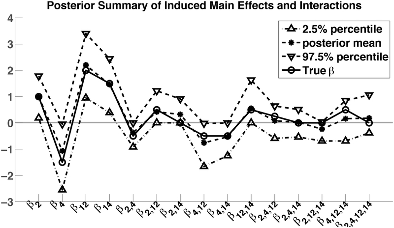
to zero. This data generating mechanism induces dependence among the variables in S*, while rendering the other variables to be marginally independent. Figure 4 reports the posterior means and 95% credible intervals for all main effects and interactions for the variables in S* averaged across 100 simulation replicates along with the true coefficients. As illustrated in Figure 4, averaging across the simulation replicates and different parameters, the 95% credible intervals cover the true parameter values 80% of the time.

Figure 4:

Posterior means and 95% credible intervals for all main effects and interactions in S* compared with the true coefficients.

Next, we study performance in estimating the dependence structure. Cramer’s V is a popular statistic measuring the strength of association or dependence between two (nominal) categorical variables in a contingency table, ranging from 0 (no association) to 1 (perfect association). Let ρ_jj′ denote the Cramer’s V statistics for variables j and j′, so that

$${\rho }_{j{j}^{\prime }}^2=\frac{1}{\text{min}\left\{d_j,d_{j^{\prime }}\right\}-1}\sum _{c_j=1}^{d_j}\sum _{c_{j^{\prime }}=1}^{d_{j^{\prime }}}\frac{{\left({\pi }_{c_j{c}_j^{\prime }}^{\left(j{j}^{\prime }\right)}-{\pi }_{c_j}^{(j)}{\pi }_{c_{j^{\prime }}}^{\left(j^{\prime }\right)}\right)}^2}{{\pi }_{c_j}^{(j)}{\pi }_{c_{\left(j^{\prime }\right)}}^{\left(j^{\prime }\right)}},$$ (18)

where ${\pi }_{l{l}^{\prime }}^{\left(j{j}^{\prime }\right)}=\text{Pr}\left(y_{ij}=l,y_{i{j}^{\prime }}=l^{\prime }\right)$ and ${\pi }_l^{(j)}=\text{Pr}\left(y_{ij}=l\right)$. Under the log-linear model (17), ρ = (ρ_jj′) is a sparse matrix with the Cramer’s V for all pairs except those in S* × S* being zero. This is an immediate consequence of the fact that if (j, j′) ∉ S* × S*, then y_ij and y_ij′, are independent.

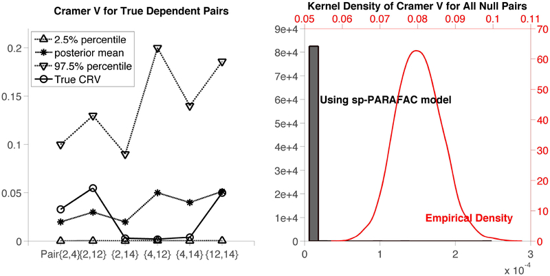
We compare estimation of the off-diagonal entries of ρ under the sp-PARAFAC model with the empirical Cramer’s V matrix $\widehat{\rho }$. We can clearly convert posterior samples for the model parameters to posterior samples for ρ_jj′ through (18). The empirical estimator is obtained by replacing ${\pi }_{c_j{c}_{j\text{'}}}^{\left(j{j}^{\prime }\right)}$ and ${\pi }_{c_j}^{(j)}$ by their empirical estimators. The left panel in Figure 5 shows the posterior summaries (averaged across simulation replicates) of the Cramer’s V values for all possible dependent pairs along with the true Cramer’s V values (which can be calculated from (17)). In the right panel of Figure 5, we overlay kernel density estimators of posterior samples (in grey) and the empirical estimators (in red) of the Cramer’s V values for all null pairs across all simulation replicates. Note the axes are also marked in grey and red for the respective cases. The sp-PARAFAC method clearly outperforms the empirical estimator convincingly, with the posterior density for the null pairs highly concentrated near zero while the empirical estimator has a mean Cramer’s V value of 0.08 across the null pairs.

Figure 5:

Left: Posterior summaries of the Cramer’s V values for all dependent pairs vs. the true Cramer’s V values; Right: Estimated density of Cramer’s V combining all null pairs under sp-PARAFAC vs. empirical estimation.

Furthermore, we can obtain power for any non-null variable or type I error for any null variable by computing the percentage of detected significance over the simulation replicates. We first look at the power and type I error of the main effects and interactions in S*, most of the power and type I error are appealing, although a few of them are far from satisfactory (see Table 2 and Table 3). However, given the Cramer’s V results in the right panel of Figure 5, the type I error for any variable not in S* should be very small or zero. As an example, we tested the main effects and all the possible interactions for positions 20, 30, 40 and 50. The type I error rates are 0 for all of them. These results are based on examining whether 95% intervals contain zero, and it is as expected that the approach may have difficulty assessing the exact interaction structure among a set of associated variables based on limited data.

Table 2:

Power for Non-null Variables Based on 100 Simulations

	β2	β4	β12	β14	β2,4	β2,12	β4,12	β4,14	β12,14	β2,4,12	β4,12,14
Power	0.97	0.9	1	1	0.95	0.99	0.98	0.97	0.99	0	0
True coefficient	1	−1.5	2	1.5	−0.5	0.5	−0.5	−0.5	0.5	0.25	0.5

Table 3:

Type I Error for Null Variables Based on 100 Simulations

	β2,4	β2,4,14	β2,12,14	β2,4,12,14
Type I error	0.97	0	0.68	0
True coefficient	0	0	0	0

5.2. Comparison with standard PARAFAC

We now conduct a simulation study to compare estimation of the Cramer’s V matrix ρ under the proposed approach to the usual specification of the PARAFAC model without any sparsity as in (4), which is equivalent to setting γ = 0 in (6). We considered 100 simulation replicates, with data in each replicate consisting of p = 100 categorical variables for n = 100 subjects, with each variable having 4 possible levels (d_j = d = 4). Two simulation settings were considered to induce dependence between the variables in S* = {2, 4, 12, 14}: (i) via multiple subpopulations as in the simulation study in Dunson and Xing (2009), and (ii) via a nominal GLM model $Pr \left(y_{ij}=c\right)=\frac{exp\left(y_{i(j)}{\beta }_c\right)}{1+{\Sigma }_{c=2}^{4}exp\left(y_{i(j)}{\beta }_c\right)}$ for j ∈ S*, where y_i(j)β_c is a linear combination of all variables that are associated with the j^th variable excluding the j^th variable. The remaining variables were independently generated from a discrete uniform distribution.

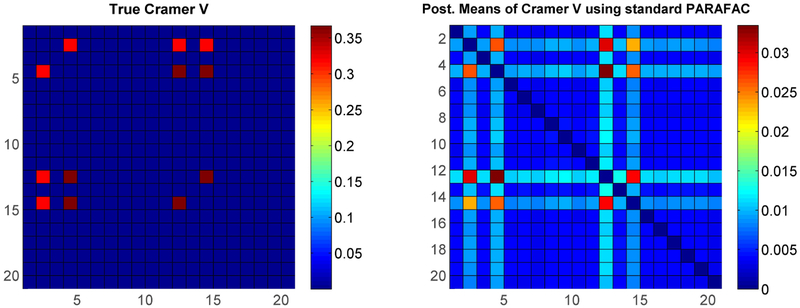
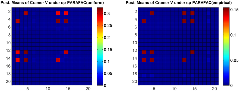
The color plot on the left in Figure 6 shows the true pairwise Cramer’s V values under simulation setting (i) (only the top-left 20 × 20 sub matrix of ρ is shown for clarity). Figure 6 (right) and Figure 7 represent one of the replicates, in which the right plot in Figure 6 shows the Cramer’s V under the standard non-sparse PARAFAC method, while Figure 7 shows the Cramer’s V using our method with two different baseline components. It is obvious that our approach has much better estimates for not only the true dependent pairs but also the true nulls. Results for simulation (ii) shown in Figure 8 again show superiority of our sparse improvement to PARAFAC.

Figure 6:

Simulation setting (i) - Left: True Cramer’s V matrix; Right: Posterior means of Cramer’s V using standard PARAFAC.

Figure 7:

Posterior means of Cramer’s V under simulation setting (i) using proposed method - Left: with ${\lambda }_0^{(j)}$ being discrete uniform; Right: with ${\lambda }_0^{(j)}$ being empirical estimates of the marginal category probabilities.

Figure 8:

Posterior means of Cramer’s V under simulation setting (ii) – Left: using standard PARAFAC; Middle: under proposed method using empirical marginal with Diri(1, …,1) prior for λ₀; Right: using proposed method with discrete uniform λ₀.

6. Application

6.1. Splice-junction Gene Sequences

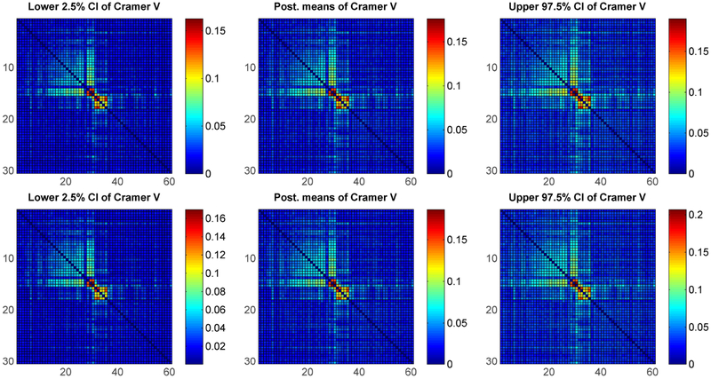
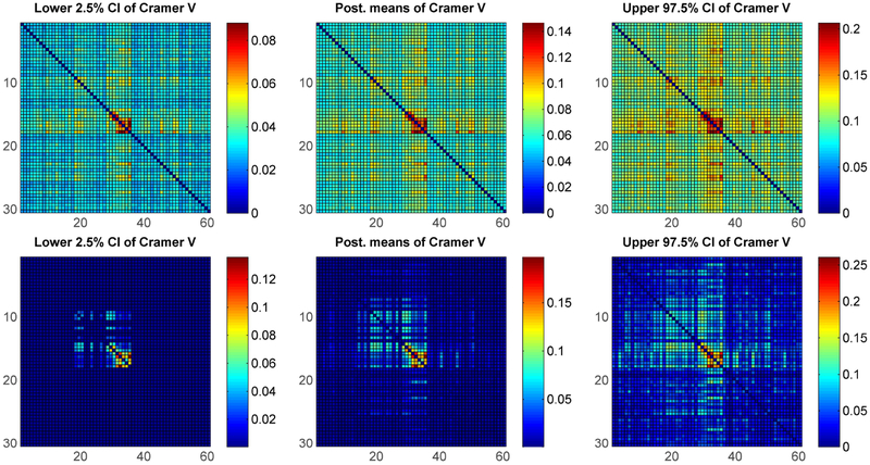
We applied the method to the Splice-junction Gene Sequences (abbreviated as splice data below). Splice junctions are points on a DNA sequence at which ‘superfluous’ DNA is removed during the process of protein creation in higher organisms. These data consist of A, C, G, T nucleotides at p = 60 positions for N = 3, 175 sequences. Since its sample size is much larger than the number of variables, we compared our approach with the standard PARAFAC in two scenarios, first a small randomly selected subset (of size n = 2p = 120) of the full data set, and second, the full data set itself. Using two different sample sizes in this manner allows for a study of the new and existing method and a comparison to a gold standard (a sufficiently large data set). We ran the analysis to estimate the pairwise positional dependence structure under the standard PARAFAC method and the proposed approach with discrete uniform baseline component. As is apparent in Figure 10, both methods have similar performance when n ≫ p, however, in the smaller sample size situation, Figure 9 demonstrates that our proposed method has the advantage of identifying the dependence structure and pushing the independent pairs to zero, which it is closer to the results in a large sample case (Figure 10).

Figure 10:

Posterior quantiles of Cramer’s V with 3,175 sequences of splice data – Upper panel: under standard PARAFAC; Bottom panel: under proposed method.

Figure 9:

Posterior quantiles of Cramer’s V with 120 sequences of splice data – Upper panel: under standard PARAFAC; Bottom panel: under proposed method.

7. Discussion

We have proposed a sparse modification to the widely-used PARAFAC tensor factorization, and have applied this in a Bayesian context to improve analyses of ultra sparse huge contingency tables. Given the compelling success in this application area, we hope that the proposed notion of sparsity will have a major impact in other areas, including tensor completion problems in machine learning. There is an enormous literature on low rank and sparse matrix factorizations, and the sp-PARAFAC should facilitate scaling of such approaches to many-way tables while dealing with the inevitable curse of dimensionality. Although we take a Bayesian approach, we suspect that frequentist penalized optimization methods can also exploit our same concept of sparsity in learning a compressed characterization of a huge array based on limited data.

Appendix

7.1. Proof of Theorem 3.1

We verify the conditions of Theorem 4 in Yang & Dunson (2013), which is a minor modification of Theorem 2 appearing in Ghosal et al. (2000). Let ϵ_n → 0 be such that $n{ϵ}_n^2\to \infty$ and ${\Sigma }_{n\ge }\text{exp}\left(-n{ϵ}_n^2\right)\le \infty$. Suppose there exist a sequence of sets ${\mathcal{P}}_n\subset {\mathcal{F}}_n$ and a constant C > 0 such that the following hold:⁴

1. $$\text{log}N\left({ϵ}_n;{\mathcal{P}}_n,\Vert \cdot {\Vert }_1\right)\le n{ϵ}_n^2$$

   $${\mathbb{P}}_n\left({\mathcal{F}}_n\cap {\mathcal{P}}_n^c\right)\le \text{exp}\left\{-(2+C)n{ϵ}_n^2\right\}$$

   $${\mathbb{P}}_n\left(\pi :\Vert \text{log}\frac{\pi }{{\pi }^{(0n)}}{\Vert }_{\infty }\le {ϵ}_n^2\right)\ge \text{exp}\left(-Cn{ϵ}_n^2\right)$$

Then, the posterior contracts at the rate ϵ_n, i.e., (8) is satisfied. We now proceed to verify conditions (1) - (3). We define,

$${\mathcal{P}}_n=\left\{\pi \in {\mathcal{F}}_n:{\pi }_{c_1\dots c_p}=\sum _{h=1}^{k_n}{\nu }_h^{*}\prod _{j\in S_h^{*}}{\lambda }_{h{c}_j}^{(*j)}\prod _{j\in S_h^{*c}}{\lambda }_{0c_j}^{(j)};\nu \in {\mathcal{S}}^{\left(k_n-1\right)},\left|S_h^{*}\right|\le A{s}_n,h=1,\dots ,k_n\right\}$$ (19)

where ${\mathcal{S}}^{(r-1)}$ denotes the (r − 1)-dimensional probability simplex and A > 0 is an absolute constant. We shall use C to denote an absolute constant whose meaning may change from one line to the next.

To estimate $N\left({ϵ}_n;{\mathcal{P}}_n,\Vert \cdot {\Vert }_1\right)$, we make use of the following Lemma, which follows in a straight-forward manner by repeated uses of the triangle inequality.

Lemma 7.1. Let π⁽¹⁾, ${\pi }^{(2)}\in {\mathcal{F}}_n$ with

$${\pi }^{(i)}=\sum _{h=1}^{k_n}{\nu }_{ih}{\lambda }_{ih}^{(1)}\otimes \dots \otimes {\lambda }_{ih}^{\left(p_n\right)},i=1,2.$$

Then,

$$\Vert {\pi }^{(1)}-{\pi }^{(2)}{\Vert }_1\le \sum _{h=1}^{k_n}\left|{\nu }_{1h}-{\nu }_{2h}\right|+\sum _{h=1}^{k_n}{\nu }_{2h}\left(\sum _{j=1}^{p_n}\sum _{c=1}^d\left|{\lambda }_{1hc}^{(j)}-{\lambda }_{2hc}^{(j)}\right|\right).$$

Lemma 7.1 implies that if π⁽¹⁾, ${\pi }^{(2)}\in {\mathcal{P}}_n$ with $S_{1h}^{*}=S_{2h}^{*}=S_h^{*}$, then

$$\Vert {\pi }^{(1)}-{\pi }^{(2)}{\Vert }_1\le \sum _{h=1}^{k_n}\left|{\nu }_{1h}-{\nu }_{2h}\right|+\sum _{h=1}^{k_n}{\nu }_{2h}\left(\sum _{j\in S_h^{*}}\sum _{c=1}^d\left|{\lambda }_{1hc}^{(j)}-{\lambda }_{2hc}^{(j)}\right|\right).$$

Based on the above observation, we create an ϵ-net of ${\mathcal{P}}_n$ as follows: In (19), (i) vary $S_h^{*}$ over all possible subsets of {1, …, p_n} with $\left|S_h^{*}\right|\le A{s}_n$ for h = 1, …, k_n, (ii) for h ∈ {1, … k_n} and $j\in S_h^{*}$, vary ${\lambda }_h^{(*j)}$ over an ϵ_n/(2Ads_n)-net of ${\mathcal{S}}^{(d-1)}$ and (iii) vary ν* over an ϵ_n/(2k_n)-net of ${\mathcal{S}}^{\left(k_n-1\right)}$.

For a fixed h, there are ${\Sigma }_{s=0}^{A{s}_n}\left(\begin{array}{l}p\hfill \\ s\hfill \end{array}\right)$ subsets of size smaller then or equal to As_n. Using the in-equality $\left(\begin{array}{l}p\hfill \\ s\hfill \end{array}\right)\le {(pe/s)}^s$ for s ≤ p/2, the number of possible subsets in (i) can be bounded above by exp(Ck_ns_n log p_n). Hence,

$$N\left({ϵ}_n;{\mathcal{P}}_n,\Vert \cdot {\Vert }_1\right)\le \text{exp}\left(C{k}_n{s}_n\text{log}{p}_n\right)N{\left({ϵ}_n/\left(2Ad{s}_n\right);{\mathcal{S}}^{d-1},\Vert \cdot {\Vert }_1\right)}^{2Ad{s}_n{k}_n}N\left({ϵ}_n/\left(2k_n\right);{\mathcal{S}}^{k_n-1},\Vert \cdot {\Vert }_1\right).$$

Using the fact that $N\left(\delta ,{\mathcal{S}}^{r-1},\Vert \cdot {\Vert }_1\right)\le {(C/\delta )}^r$ (Vershynin, 2010), the right hand side in the above display can be bounded above by $\text{exp}\left(C{s}_n\text{log}{p}_n\right)=\text{exp}\left(n{ϵ}_n^2\right)$, since k_n = O(1).

We now bound ${\mathbb{P}}_n\left({\mathcal{F}}_n\cap {\mathcal{P}}_n^c\right)$. Recall that in the sp-PARAFAC model, the induced prior on the subset size |S_h| is Bin(p_n, τ_h), with τ_h ~ Beta(1, γ). Now,

$${\mathbb{P}}_n(\left({\mathcal{F}}_n\cap {\mathcal{P}}_n^c\right)\le \text{ Pr}\left(\exists h\in \left\{1,\dots ,k_n\right\}\text{s.t. }\left|S_h\right|\ge A{s}_n\right)\le k_{n}P\left(\left|S_1\right|>A{s}_n\right).$$

Integrating τ₁, the distribution of |S₁| is a beta-bernoulli distribution with probability mass function

$$\text{Pr }\left(\left|S_1\right|=s\right)=\left(\begin{array}{c}p\\ s\end{array}\right)\frac{1}{\text{B}(1,\gamma )}{\int }_{\tau =0}^1{\tau }^s{(1-\tau )}^{p_n-s}{(1-\tau )}^{\gamma -1}d\tau =\left(\begin{array}{c}{p}_n\\ s\end{array}\right)\frac{\text{B}\left(1+s,\gamma +p_n-s\right)}{\text{B}(1,\gamma )}=\frac{1}{\gamma }\frac{p_n!}{\left(p_n-s\right)!}\frac{\left(\gamma +p_n-s-1\right)!}{\left(\gamma +p_n\right)!},$$

for s = 0,1,…, p_n. B(·, ·) denotes the Beta function in the above display. Hence, for s ≥ 1,

$$\frac{\text{ Pr}\left(\left|S_1\right|=s\right)}{\text{ Pr}\left(\left|S_1\right|=s-1\right)}=\frac{\left(p_n-s+1\right)}{\left(p_n-s+\gamma \right)}.$$

Now, letting $\gamma =p_n^2$, one has for any p_n ≥ 2 and 1 ≤ s ≤ p_n/2,

$$\frac{1}{4p_n}\le \frac{\left(p_n-s+1\right)}{\left(p_n-s+\gamma \right)}\le \frac{1}{p_n}.$$

In general, for $\gamma =\beta p_n^2$, we can bound this from both sides by C/p_n. Noting that $\text{Pr}\left(\left|S_1\right|=0\right)=C/p_n^3$, we have

$$\text{Pr}\left(\left|S_1\right|=s\right)=\frac{C}{p_n^3}\prod _{j=1}^s\frac{\text{ Pr}\left(\left|S_1\right|=j\right)}{\text{ Pr}\left(\left|S_1\right|=j-1\right)},$$

implying there exists constants c₁, c₂ > 0 such that

$$e^{-c_1(s+3)\text{log}{p}_n}\le \text{Pr}\left(\left|S_1\right|=s\right)\le e^{-c_2(s+3)\text{log}{p}_n},$$ (20)

for 0 ≤ s ≤ p_n/2. In particular, the upper bound holds for all 0 ≤ s ≤ p_n, since (p_n − s + 1)/(p_n − s + γ) ≤ C/p_n for all s. Hence, for n large enough so that s_n ≥ 3,

$$\text{P}\left(\left|S_1\right|>A{s}_n\right)\le \sum _{j=A{s}_n+1}^{p_n}\text{exp}\left(-Cj\text{log}{p}_n\right)\le \text{exp}\left(-C{s}_n\text{log}{p}_n\right)\le \text{exp}\left(-n{ϵ}_n^2\right).$$

We finally show that (3) holds. Recall the decomposition of π⁽⁰ⁿ⁾ from (9). A probability tensor π following a sp-PARAFAC model with a truncated stick-breaking prior on ν can be parameterized as

$${\theta }_{\pi }=\left(\nu ,{\left\{S_h\right\}}_{1\le h\le k_n},{\left\{{\lambda }_h^{(j)}\right\}}_{1\le h\le k_n,j\in S_h}\right),$$

where $\nu \in {\mathcal{S}}^{k_n-1}$, S_h ⊂ {1, …, p_n}, ${\lambda }_h^{(j)}\in {\mathcal{S}}^{d-1}$. Consider the following subset $\mathcal{A}$ of the parameter space,

$$\mathcal{A}=\left\{S_h=S_0,1\le h\le k_n;\sum _{h=1}^{k_n}\left|{\nu }_h-{\nu }_{0h}\right|\le \frac{{ϵ}_n^2}{2e^{c_0{s}_n}};\sum _{c=1}^d\left|{\lambda }_{hc}^{(j)}-{\overline{\lambda }}_{hc}^{(0j)}\right|\le \frac{{ϵ}_n^2{\epsilon }_0}{4q_n},1\le h\le k_n,j\in S_0\right\}.$$

We now show that ${\theta }_{\pi }\in \mathcal{A}$ implies $\text{log}\Vert \pi /{\pi }^{(0n)}{\Vert }_{\infty }\le {ϵ}_n^2$, so that ${\mathbb{P}}_n\left(\text{log}\Vert \pi /{\pi }^{(0n)}{\Vert }_{\infty }\le {ϵ}_n^2\right)$ can be bounded below by ${\mathbb{P}}_n(\mathcal{A})$. First, observe that since S_h = S₀ for all h on $\mathcal{A}$, π/π⁽⁰ⁿ⁾ = ψ/ψ⁽⁰ⁿ⁾, where ψ⁽⁰ⁿ⁾ is as in (10) and ψ is the d^qn joint probability tensor implied by the sp-PARAFAC model for the variables {y_ij : j ∈ S₀},

$${\psi }_{c_1\dots c_{q_n}}=\sum _{h=1}^{k_n}{\nu }_h\prod _{j\in S_0}{\lambda }_{h{c}_j}^{\left(e_j\right)}.$$

Hence,

$$\text{log}{\Vert \frac{\pi }{{\pi }^{(0n)}}\Vert }_{\infty }=\text{log}{\Vert \frac{\psi }{{\psi }^{(0n)}}\Vert }_{\infty }\le \text{log}\left(1+{\Vert \left(\frac{\psi }{{\psi }^{(0n)}}-1\right)\Vert }_{\infty }\right)\le {\Vert \left(\frac{\psi }{{\psi }^{(0n)}}-1\right)\Vert }_{\infty },$$

where the penultimate step follows from an application of triangle inequality and the last step uses log(1 + x) ≤ x for x ≥ 0. For any $c_1,\dots ,c_{s_n}$, by an application of triangle inequality,

$$\left|{\psi }_{c_1\dots c_{s_n}}-{\psi }_{c_1\dots c_{sn}}^{(0n)}\right|\le \sum _{h=1}^{k_n}\left|{\nu }_h-{\nu }_{0h}\right|+\sum _{h=1}^{k_n}{\nu }_{0h}\left|\prod _{j=1}^{q_n}{\lambda }_{h{c}_j}^{\left(e_j\right)}-\prod _{j=1}^{q_n}{\overline{\lambda }}_{h{c}_j}^{\left(0e_j\right)}\right|.$$ (21)

We now state a Lemma to facilitate bounding the second term of the above display.

Lemma 7.2. Let v₁,… v_r ∈ (ε₀, 1 − ε₀) for some ε₀ > 0. Let δ > 0 be such that rδ < ε₀/2. Then, if u₁, …, u_r satisfy |u_j − v_j | ≤ δ for all j = 1, …, r, then

$$\left|u_1\dots u_r-v_1\dots v_r\right|\le \frac{2r\delta }{{\epsilon }_0}{v}_1\dots v_r.$$

Apply Lemma 7.2 with r = q_n, $u_j={\overline{\lambda }}_{h{c}_j}^{\left(0e_j\right)}$ and $\delta ={ϵ}_n^2{\epsilon }_0/\left(4q_n\right)$ (clearly $r\delta /{\epsilon }_0={ϵ}_n^2/4<1/2$) to obtain that for any 1 ≤ h ≤ q_n, $\left|{\Pi }_{j=1}^{q_n}{\lambda }_{h{c}_j}^{\left(e_j\right)}-{\Pi }_{j=1}^{q_n}{\overline{\lambda }}_{h{c}_j}^{\left(0e_j\right)}\right|\le \left({ϵ}_n^2/2\right){\Pi }_{j=1}^{q_n}{\overline{\lambda }}_{h{c}_j}^{\left(0e_j\right)}$.·Substituting this bound in (21), we have on $\mathcal{A}$,

$$\frac{\left|{\psi }_{c_1\dots c_{s_n}}-{\psi }_{c_1\dots c_{s_n}}^{(0n)}\right|}{{\psi }_{c_1\dots c_{s_n}}^{(0n)}}\le \frac{{\Sigma }_{h=1}^{k_n}\left|{\nu }_h-{\nu }_{0h}\right|}{e^{-c_0{s}_n}}+\left({ϵ}_n^2/2\right)\frac{{\Sigma }_{h=1}^{k_n}{\nu }_{0h}{\Pi }_{j=1}^{q_n}{\overline{\lambda }}_{h{c}_j}^{\left(0e_j\right)}}{{\psi }_{c_1\dots c_{s_n}}^{(0n)}}\le {ϵ}_n^2.$$

For the two terms in the above display after the first inequality, we used the lower bound (11) for the first term along with ${\Sigma }_{h=1}^{k_n}\left|{\nu }_h-{\nu }_{0h}\right|\le {ϵ}_n^2/\left(2e^{c_0{s}_n}\right)$ on $\mathcal{A}$, and by definition of ψ⁽⁰ⁿ⁾, the second term is ${ϵ}_n^2/2$.

It thus remains to lower bound ${\mathbb{P}}_n(\mathcal{A})$. By independence across h, $\text{Pr}\left(S_h=S_0,1\le h\le k_n\right)=\text{Pr}{\left(S_1=S_0\right)}^{k_n}$. Further, by exchangeability of the prior on S₁, since all subsets of a particular size receive the same prior probability, $Pr \left(S_1=S_0\right)= Pr \left(\left|S_1\right|=q_n\right)/\left(\begin{array}{l}{p}_n\hfill \\ q_n\hfill \end{array}\right)$. From (20), Pr(|S₁| = q_n ≥ exp(−Cs_n log p_n). Using $\left(\begin{array}{l}{p}_n\hfill \\ q_n\hfill \end{array}\right)\le {\left(p_{n}e/q_n\right)}^{q_n}$, we conclude that Pr(S₁ = S₀) ≥ exp(−Cs_n log p_n).

Recall that ${\nu }_h={\nu }_h^{*}{\Pi }_{l<h}\left(1-{\nu }_l^{*}\right)$, where ${\nu }_l^{*}~\text{Beta}(1,\alpha )$ independently. Find numbers {${\nu }_{0h}^{*}$} such that ${\nu }_{0h}={\nu }_{0h}^{*}{\Pi }_{l<h}\left(1-{\nu }_{0l}^{*}\right)$. It is easy to see that there exists a constant C > 0 such that $\left|{\nu }_h^{*}-{\nu }_{0h}^{*}\right|\le {ϵ}_n/\left(C{k}_n\right)$ for all h = 1, …, k_n implies ${\Sigma }_{h=1}^{k_n}\left|{\nu }_h-{\nu }_{0h}\right|\le {ϵ}_n$. Hence, using a general result on small ball probability estimate of Dirichlet random vectors (Lemma 6.1 of Ghosal et al. (2000)), one has

$$\text{Pr}\left(\sum _{h=1}^{k_n}\left|{\nu }_h-{\nu }_{0h}\right|\le \frac{{ϵ}_n^2}{2e^{c_0{s}_n}}\right)\ge \text{exp}\left\{-C{s}_n\text{log}\left(1/{ϵ}_n\right)\right\}.$$

Again, applying Lemma 6.1 of Ghosal et al. (2000),

$$Pr \left(\sum _{c=1}^d\left|{\lambda }_{hc}^{(j)}-{\overline{\lambda }}_{hc}^{(0j)}\right|\le \frac{{ϵ}_n^2{\epsilon }_0}{4q_n}\right)\ge \text{exp}\left\{-C\text{log}\left(s_n/{ϵ}_n\right)\right\}.$$

Combining, we get $Pr (\mathcal{A})\ge \text{exp}\left(-C{s}_n\text{log}{p}_n\right)\ge \text{exp}\left(-n{ϵ}_n^2\right)$. Hence, we have established (1) - (3) completing the proof.

7.2. Proof of Lemma 7.2

Observe that

$$\left|u_1\dots u_r-v_1\dots v_r\right|=\left|v_1\dots v_r\right|\left|\frac{u_1\dots u_r}{v_1\dots v_r}-1\right|=v_1\dots v_r\text{max}\left\{\frac{u_1\dots u_r}{v_1\dots v_r}-1,1-\frac{u_1\dots u_r}{v_1\dots v_r}\right\}.$$

Now, since u_h ≤ v_h + δ for all h,

$$\frac{u_1\dots u_r}{v_1\dots v_r}\le \prod _{h=1}^r\left(1+\delta /v_h\right)\le {\left(1+\delta /{\epsilon }_0\right)}^r.$$

Using the binomial theorem, ${\left(1+\delta /{\epsilon }_0\right)}^r-1=r\delta /{\epsilon }_0+{\Sigma }_{h=2}^r\left(\begin{array}{l}r\hfill \\ h\hfill \end{array}\right){\left(\delta /{\epsilon }_0\right)}^h$. Next, bound $\left(\begin{array}{l}r\hfill \\ h\hfill \end{array}\right)\le r^h$ and use the fact that rδ/ε₀ < 1/2 to conclude that ${\Sigma }_{h=2}^r\left(\begin{array}{l}r\hfill \\ h\hfill \end{array}\right){\left(\delta /{\epsilon }_0\right)}^h\le {\Sigma }_{h=1}^{\infty }{\left(r\delta /{\epsilon }_0\right)}^h\le 2r\delta /{\epsilon }_0$.

On the other hand, using u_h ≥ v_h − δ for all h,

$$\frac{u_1\dots u_r}{v_1\dots v_r}\ge \prod _{h=1}^r\left(1-\delta /v_h\right)\ge {\left(1-\delta /{\epsilon }_0\right)}^r\ge 1-r\delta /{\epsilon }_0.$$

The proof is concluded by observing that

$$\text{max}\left\{\frac{u_1\dots u_r}{v_1\dots v_r}-1,1-\frac{u_1\dots u_r}{v_1\dots v_r}\right\}\le 2r\delta /{\epsilon }_0.$$

References

- Agresti A (2002), Categorical data analysis, Vol. 359, Wiley-interscience. [Google Scholar]
- Armagan A, Dunson D, and Lee J (2013a), “Generalized double Pareto shrinkage,” Statistica Sinica, 23, 119–143. [PMC free article] [PubMed] [Google Scholar]
- Armagan A, Dunson D, Lee J, Bajwa W, and Strawn N (2013b), “Posterior consistency in high-dimensional linear models,” Biometrika (to appear). [Google Scholar]
- Belitser E, and Ghosal S (2003), “Adaptive Bayesian inference on the mean of an infinitedimensional normal distribution,” The Annals of Statistics, 31, 536–559. [Google Scholar]
- Bhattacharya A, and Dunson D (2011), “Sparse Bayesian infinite factor models,” Biometrika, 98, 291–306. [DOI] [PMC free article] [PubMed] [Google Scholar]
- Bhattacharya A, and Dunson D (2012), “Simplex factor models for multivariate unordered categorical data,” Journal of the American Statistical Association, 107, 362–377. [DOI] [PMC free article] [PubMed] [Google Scholar]
- Bontemps D (2011), “Bernstein-von Mises theorems for Gaussian regression with increasing number of regressors,” The Annals of Statistics, 39, 2557–2584. [Google Scholar]
- Bro R (1997), “PARAFAC. Tutorial and applications,” Chemometrics and Intelligent Laboratory Systems, 38, 149–171. [Google Scholar]
- Candes E, and Recht B (2009), “Exact matrix completion via convex optimization,” Foundations of Computational Mathematics, 9, 717–772. [Google Scholar]
- Carvalho C, Lucas J, Wang Q, Nevins J, and West M (2008), “High-dimensional sparse factor modelling: applications in gene expression genomics,” Journal of the American Statistical Association, 103, 1438–1456. [DOI] [PMC free article] [PubMed] [Google Scholar]
- Carvalho C, Polson N, and Scott J (2010), “The horseshoe estimator for sparse signals,” Biometrika, 97, 465–480. [Google Scholar]
- Castillo I, and van der Vaart A (2012), “Needles and straws in a haystack: Posterior concentration for possibly sparse sequences,” The Annals of Statistics, 40, 2069–2101. [Google Scholar]
- Chartrand R (2012), “Nonconvex splitting for regularized low-rank plus sparse decomposition,” IEEE Transactions on Signal Processing, 60, 5810–5819. [Google Scholar]
- Dunson DB, and Xing C (2009), “Nonparametric Bayes modeling of multivariate categorical data,” Journal of the American Statistical Association, 104, 1042–1051. [DOI] [PMC free article] [PubMed] [Google Scholar]
- Fienberg S, and Rinaldo A (2007), “Three centuries of categorical data analysis: Log-linear models and maximum likelihood estimation,” Journal of Statistical Planning and Inference, 137, 3430–3445. [Google Scholar]
- Friedlander M, and Hatz K (2005), “Computing non-negative tensor factorizations,” Optimization Methods and Software, 23, 631–647. [Google Scholar]
- Ge Y, and Jiang W (2006), “On consistency of Bayesian inference with mixtures of logistic regression,” Neural Computation, 18, 224–243. [DOI] [PubMed] [Google Scholar]
- Gelman A, Jakulin A, Pittau M, and Su Y (2008), “A weakly informative default prior distribution for logistic and other regression models,” Annals of Applied Statistics, 2, 1360–1383. [Google Scholar]
- Ghosal S (1999), “Asymptotic normality of posterior distributions in high-dimensional linear models,” Bernoulli, 5, 315–331. [Google Scholar]
- Ghosal S (2000), “Asymptotic normality of posterior distributions for exponential families when the number of parameters tends to infinity,” Journal of Multivariate Analysis, 74, 49–68. [Google Scholar]
- Ghosal S, Ghosh J, and van der Vaart A (2000), “Convergence rates of posterior distributions,” Annals of Statistics, 28, 500–531. [Google Scholar]
- Hans C (2011), “Elastic net regression modeling with the orthant normal prior,” Journal of the American Statistical Association, 106, 1383–1393. [Google Scholar]
- Harshman R (1970), “Foundations of the PARAFAC procedure: Models and conditions for an “explanatory” multi-modal factor analysis,” UCLA Working Papers in Phonetics, 16, 84. [Google Scholar]
- Jiang W (2007), “Bayesian variable selection for high dimensional generalized linear models: convergence rates of the fitted densities,” The Annals of Statistics, 1487–1511. [Google Scholar]
- Karatzoglou A, Amatriain X, Baltrunas L, and Oliver N (2010), “Multiverse recommendation: n-dimensional tensor factorization for context-aware collaborative filtering,” Proceedings of the Fourth ACM Conference on Recommender Systems. [Google Scholar]
- Kolda T, and Bader B (2009), “Tensor decompositions and applications,” SIAM Review, 51, 455–500. [Google Scholar]
- Lee DD, and Seung HS (1999), “Learning the parts of objects by non-negative matrix factorization,” Nature, 401,788–791. [DOI] [PubMed] [Google Scholar]
- Lim L, and Comon P (2009), “Nonnegative approximations of nonnegative tensors,” Jour. Chemometrics, 432–441. [Google Scholar]
- Liu J, Liu J, Wonka P, and Ye J (2012), “Sparse non-negative tensor factorization using column-wise coordinate descent,” Pattern Recognition, 45, 649–656. [Google Scholar]
- Lucas JE, Carvalho C, Wang Q, Bild A, Nevins J, and West M (2006), “Sparse statistical modelling in gene expression genomics,” in Bayesian Inference for Gene Expression and Proteomics, eds. Do K, Müller P and Vannucci M, Cambridge University Press, pp. 155–176. [Google Scholar]
- Paatero P, and Tapper U (1994), “Positive matrix factorization: A non-negative factor model with optimal utilization of error estimates of data values,” Environmetrics, 5, 111–126. [Google Scholar]
- Park T, and Casella G (2008), “The Bayesian lasso,” Journal of the American Statistical Association, 103,681–686. [Google Scholar]
- Pati D, Bhattacharya A, Pillai N, and Dunson D (2013a), “Posterior contraction in sparse Bayesian factor models for massive covariance matrices,” arXiv:1206.3627. [Google Scholar]
- Pati D, Dunson DB, and Tokdar ST (2013b), “Posterior consistency in conditional distribution estimation,” Journal of Multivariate Analysis. [DOI] [PMC free article] [PubMed] [Google Scholar]
- Polson N, and Scott J (2010), “Shrink globally, act locally: Sparse Bayesian regularization and prediction,” in Bayesian Statistics 9 (Bernardo JM, Bayarri MJ, Berger JO, Dawid AP, Heckerman D, Smith AFM and West M, eds.), Oxford University Press, New York, pp. 501–538. [Google Scholar]
- Scott J, and Berger J (2010), “Bayes and empirical-Bayes multiplicity adjustment in the variable selection problem,” The Annals of Statistics, 38, 2587–2619. [Google Scholar]
- Sethuraman J (1994), “A constructive definition of Dirichlet priors,” Statistica Sinica, 4, 639–650. [Google Scholar]
- Shen W, Tokdar S, and Ghosal S (2011), “Adaptive Bayesian multivariate density estimation with Dirichlet mixtures,” arXivpreprint arXiv:1109.6406. [Google Scholar]
- Talagrand M (1996), “A new look at independence,” The Annals of Probability, 24, 1–34. [Google Scholar]
- van der Vaart A, and van Zanten J (2008), “Rates of contraction of posterior distributions based on Gaussian process priors,” The Annals of Statistics, 36, 1435–1463. [Google Scholar]
- Vershynin R (2010), “Introduction to the non-asymptotic analysis of random matrices,” Arxiv preprint arxiv:1011.3027. [Google Scholar]
- West M (2003), “Bayesian factor regression models in the “large p, small n” paradigm,” in Bayesian Statistics 7 (Bernardo JM, Bayarri MJ, Berger JO, Dawid AP, Heckerman D, Smith AFM and West M, eds.), Oxford University Press, New York, pp. 733–742. [Google Scholar]
- Yang Y, and Dunson DB (2013), “Bayesian conditional tensor factorizations for high-dimensional classification,” arXiv preprint arXiv:1301.4950. [DOI] [PMC free article] [PubMed] [Google Scholar]