Decoding phonation with artificial intelligence (DeP AI): Proof of concept

Abstract

Objective

Acoustic analysis of voice has the potential to expedite detection and diagnosis of voice disorders. Applying an image‐based, neural‐network approach to analyzing the acoustic signal may be an effective means for detecting and differentially diagnosing voice disorders. The purpose of this study is to provide a proof‐of‐concept that embedded data within human phonation can be accurately and efficiently decoded with deep learning neural network analysis to differentiate between normal and disordered voices.

Methods

Acoustic recordings from 10 vocally‐healthy speakers, as well as 70 patients with one of seven voice disorders (n = 10 per diagnosis), were acquired from a clinical database. Acoustic signals were converted into spectrograms and used to train a convolutional neural network developed with the Keras library. The network architecture was trained separately for each of the seven diagnostic categories. Binary classification tasks (ie, to classify normal vs. disordered) were performed for each of the seven diagnostic categories. All models were validated using the 10‐fold cross‐validation technique.

Results

Binary classification averaged accuracies ranged from 58% to 90%. Models were most accurate in their classification of adductor spasmodic dysphonia, unilateral vocal fold paralysis, vocal fold polyp, polypoid corditis, and recurrent respiratory papillomatosis. Despite a small sample size, these findings are consistent with previously published data utilizing deep neural networks for classification of voice disorders.

Conclusion

Promising preliminary results support further study of deep neural networks for clinical detection and diagnosis of human voice disorders. Current models should be optimized with a larger sample size.

Levels of Evidence

Level III

INTRODUCTION

The clinical diagnosis of voice disorders relies on both the physical examination of laryngeal function and perceptual assessment of the acoustic output. While physical examination via endoscopy is the current gold standard for diagnosis, laryngoscopy and/or stroboscopy requires clinical expertise, and limited access to these clinical specialists may delay diagnosis. Perceptual assessment based on sound encoded within the voice signal is noninvasive, easily acquired, and has the potential to accelerate and/or confirm diagnosis; however, perceptual assessment of voice quality is subjective, and inter‐ and intra‐rater reliability is highly influenced by clinician background, training, and experience.1

Acoustic analysis via instrumentation was initially introduced in the early 1990s as a quantitative means to measure acoustic deviations from normal voice production.2 Despite its widespread use for screening and progress monitoring, intrinsic limitations have prevented its effective application for automated detection and diagnosis of voice disorders.3 Acoustic analysis has traditionally relied on the characterization of limited numbers of acoustic parameters.4 The mechanism of human speech production is highly complex, however, and any given pathology affects multiple acoustic parameters simultaneously. Although a highly trained expert human brain can integrate and interpret these multiple deviations to identify the presence of voice disorders and inform differential diagnosis, a parameter‐by‐parameter approach to acoustic analysis has not replicated this functionality.

Artificial intelligence using deep neural networks may provide an alternative to the single or multidimensional parameter approach to acoustic analysis. Neural network learning has been extensively developed for automatic speech recognition applications since the 1980s.4 Despite extensive research developing deep learning architectures to decode the speech signal for linguistic content, only a few studies have applied this technology to analysis of the disordered voice. Findings from these studies, which report disorder‐based classification accuracies for dysphonic voices between 40% and 96%, support the value of using deep neural networks for detection and differential diagnosis of voice disorders.5, 6, 7 These studies, however, not only require analysis of multiple acoustic parameters, which slows processing times, but they also rely heavily on the Mel frequency cepstral coefficient (MFCC), which filters frequency data to maintain the long‐term temporal aspects of the frequency spectrum needed to extract critical linguistic elements of the speech signal. While this discarded frequency data may not be salient for speech recognition, it may be vital for the detection of and distinction between certain voice disorders.

Recent studies have recommended moving away from the MFCC in favor of spectrograms.8, 9 Not only do spectrograms maintain the full frequency resolution of the acoustic signal, but they also have the unique characteristic of being data‐rich images that can be analyzed via image analysis techniques. Since the early 2010s, a revolution in the field of image analysis has occurred. Tasks like image classification have been solved with near‐human levels of accuracy.5 Within medicine, image analysis with a neural network approach has made inroads into clinical diagnostics in both radiology10 and dermatology,11 ultimately expediting accurate diagnoses using noninvasive techniques.

We hypothesize that applying an image‐based neural network approach to classify voice disorders may result in similar advancements in laryngology. The overarching goal of this line of research is to develop a deep neural network application that is sensitive to deviations from normal voice production and can simultaneously integrate these deviations across a variety of voice characteristics to provide an accurate differential diagnosis that can equal or exceed the accuracy of current instrumental or perceptual assessment techniques. As a first step in this process, the purpose of this study is to provide a proof‐of‐concept that embedded data within human phonation can be accurately and efficiently decoded with deep learning neural network analysis to differentiate between normal and disordered voices.

MATERIALS AND METHODS

This study was performed in accordance with the Declaration of Helsinki, Good Clinical Practice, and was approved by the Institutional Review Board at Vanderbilt University Medical Center (IRB#: 181191). The study utilized previously collected acoustic recordings from patients with voice disorders, as well as vocally healthy individuals. As part of standard of care, individuals seen at the Vanderbilt Voice Center with a voice complaint are asked to provide a standardized voice sample. These voice samples are captured at the time of evaluation and stored on a secure server (ImageStream, Image Stream Medical, Littleton, MA) as part of the patient's electronic medical record. Voice samples from vocally healthy individuals are also included in this electronic database as reference.

Data Collection

Participants

Ten vocally healthy adults and 70 adults with voice disorders were included in this study. The mean age of the vocally healthy participants (8 female, 2 male) was 34 (SD = 10); the mean age of the participants with voice disorders (47 female, 23 male) was 56 (SD = 16). Participants were identified by querying the electronic database by either diagnosis or normal voice status. The following diagnoses were included in the study (the sample size is n = 10 in each diagnostic group): adductor spasmodic dysphonia (ADSD), essential tremor of voice (ETV), muscle tension dysphonia (MTD), polypoid corditis or Reinke's edema (PCord), unilateral vocal fold paralysis (UVFP), vocal fold polyp (Polyp), and recurrent respiratory papillomatosis (RRP). Diagnoses were confirmed by two independent, board‐certified laryngologists at the Vanderbilt Voice Center. While not comprehensive, these diagnostic categories represent commonly treated disorders at the Vanderbilt Voice Center, and thus serve as a reasonable starting point for this proof of concept study.

Acoustic recordings

All participants were recorded reading the first three sentences of the phonetically balanced Rainbow Passage.12 Recordings were obtained in a quiet clinic room using an omnidirectional lapel microphone with a 44.1‐kHz sampling rate (Olympus Visera Elite OTV‐S19; Olympus Medical, Center Valley, PA) and stored on the clinical server as .mp4 files with audio compressed at 186 kbps. Using the open‐source audio editor Audacity (Audacity v2.2.1, 2017), the acoustic signals were extracted from the video files, edited to include only the Rainbow Passage, and saved as uncompressed .wav files (dual channels, 8 bits per channel) in a password‐protected, REDCap database.

Data processing

Validation Set

To augment the limited amount of data in the validation set, as well as make the model's predictions more robust, the raw .wav files were segmented into 3‐second, non‐overlapping “chunks.”13 For the last chunk of each recording (which would not be a full 3 seconds), the chunk's frequencies were repeated with a small amount of noise (<5%) until the 3‐second window was filled. While the source audio captures frequencies up to 22.5 kHz, the frequency ceiling for the images was set at 8 kHz in order to provide better resolution of relevant voice data and remove any compression artifact; therefore, the frequency range represented in the acoustic signal was 0 to 8 kHz. Following segmentation, all .wav files were transformed into grayscale, wide‐band, linear spectrograms (8‐bit depth per channel) using the short‐time Fourier transform (as shown in Figure 1) with a block‐size of 2048 data points and overlap of 1536, or 75%, so as to increase the resolution and smoothness of the resulting images. Since the audio recordings were segmented into 3‐second chunks, each raw spectrogram was scaled by an 8/3 ratio at 1 inch/second, in order to obtain a final png image size of 256x256 pixels with a resolution of 96 dots/inch. These techniques standardized the spectrograms in both the frequency and time domains for input to the neural network. Table 1 details the breakdown of total number of spectrograms for each diagnostic group within the validation set.

Figure 1.

To standardize input into the neural network, acoustic signals were segmented into 3‐second chunks (left) and transformed into spectrograms using the Fourier transform (middle). Spectrograms displayed frequency over time, with intensity coded by grayscale (right).

Table 1.

Total Sample Size for Each Group and the Derived Baseline Accuracy for Each Classification Task.

Diagnostic Group	Normal	ADSD	ETV	MTD	PCord	UVFP	Polyp	RRP	Total
Total Spectrograms	45	56	74	49	54	59	56	58	451
Baseline Accuracy
Naïve algorithm (%)	–	56/101 (55%)	74/119 (62%)	49/94 (52%)	54/99 (55%)	59/104 (57%)	56/101 (55%)	58/103 (56%)	–

Normal = vocally healthy; AdSD = adductor spasmodic dysphonia; ETV = essential tremor of voice; MTD = muscle tension dysphonia; Pcord = polypoid corditis or Reinke's edema; Polyp = vocal fold polyp; RRP = recurrent respiratory papillomatosis; UVFP = unilateral vocal fold paralysis.

Training Set

Large data sets (preferably made up of thousands of images with balanced classes) are necessary to provide sufficient material to train deep learning models. Consequently, data augmentation techniques are commonly employed to increase the size of the training set when sample sizes are small. A common augmentation technique boosts model performance by introducing random rotations and scalings of the original images13; however, this technique is inappropriate for the current application due to the inherent symmetry of the sound spectrogram images. The spectrogram is a two‐dimensional visual representation of the frequency and intensity spectrums; all the spikes are parallel to the frame borders and are therefore relevant for this specific classification task. As such, the interpretation of the image is highly dependent on the orientation of the image and thus the orientation cannot be varied. However, neural networks can also recognize salient elements independent of the position in the image. Therefore, to augment the sample size of the training set, each organic spectrogram was randomly divided with a single, vertical splice and the subsequent pieces were reversed in order to create a new 3‐second spectrogram. This process was repeated 10 times for each spectrogram, rendering a synthetic training set of 4510 images.

Data Exploration

Model development

An open‐source, deep‐learning library named Keras was used for this study.14 The Keras library is written in Python and was selected due to its ease of use and flexible interface that allows a combination of different types of layers in non‐sequential architectures, with heterogeneous inputs and outputs.15 Figure 2 shows the architecture of the convolutional neural network deep learning model used for the binary classification tasks, built in Keras.14 The dimensions and number of parameters of each layer are shown, with a total of 6 795 457 parameters. The network is a Convolutional Neural Network (CNN) with a dropout used to reduce overfitting (when the model learns the training data too well, resulting in poor generalization) by means of regularization. CNNs are a special kind of neural network inspired by how the human brain perceives and classifies objects. The network works by taking an image and reducing it to simpler features that the computer can work with (such as edges and color spots) through a series of convolutions and pooling operations (Fig. 2, Conv2D, and MaxPooling2D). The spatial information from the original image is preserved during these convolutions so that in the final layers, these features are combined together to produce a feature map. The network assigns a probability that the image belongs to a certain class based on the data it has previously been trained on.

Figure 2.

Summary of the Keras convolutional neural network models trained for the seven binary classification tasks. Conv2D = 2D convolutional layer; MaxPooling2D = 2D max‐pooling layer.

Model validation

Given the small size of the whole data set consisting of only 451 images (Table 1), we chose to perform a 10‐fold cross validation to evaluate our models. All images corresponding to an individual subject belonged to the same fold to ensure independence between folds, preventing leakage of information from the training set to the validation set. In other words, for the classification problem corresponding to each disease, each fold contained all the spectrograms corresponding to one subject having the disease, and all the spectrograms corresponding to a normal subject. For example, the frames used in the fifth validation fold include all spectrograms from the fifth normal subject and the fifth ADSD patient. Figure 3 shows the spectrograms from all normal subjects (left) and all patients with ADSD (right), the spectrograms included in the fifth validation fold are surrounded by a dashed line. This neural network was trained on the synthetic images derived from all the other organic spectrogram frames in Figure 3 and was then used to perform the binary classification task on the frames surrounded by black lines. For each iteration of the model, the organic and synthetic images from the sequential folds were withheld from the training set for validation. Each fold (including both organic and synthetic images) was therefore incorporated into the training set nine times and the organic images served as the validation set once. This technique was employed to ensure some statistical significance in the results, which is even more necessary in this case of little data available.

Figure 3.

Spectrograms of all audio files from vocally healthy individuals (left) and patients with adductor spasmodic dysphonia (right). The fifth validation fold classified all spectrograms from normal subject 5 and ADSD patient 5. Frames used in the binary classification task are surrounded by lines. Synthetic images derived from all other organic spectrograms were used to train the model. ADSD = adductor spasmodic dysphonia.

Binary classification tasks

Seven binary classification tasks were conducted to categorize normal and disordered voice samples. These classification tasks mimicked a clinical screening task to discriminate between normal and disordered for each of the seven diagnostic groups. The network architecture of the deep learning model (shown in Figure 2) was trained separately for each fold within each of the seven diagnostic groups, for a total of 70 models. Training for each model required 10 full presentations of the data (epochs), which were iteratively optimized using gradient descent with 100 backpropagation steps and a learning rate equal to 10‐4.

The primary metric for assessing our training was accuracy, defined as the fraction of all correctly classified instances with respect to the total number of instances. Baseline accuracy (the minimally acceptable level of accuracy) for each disorder was determined by a naïve algorithm that always predicted the disordered class ($\mathit{\text{Baseline accuracy}}=\frac{{\mathit{\text{Spect}}}_D}{{\mathit{\text{Spect}}}_N+{\mathit{\text{Spect}}}_D}$, where Spect_D is the total number of disordered frames, and Spect_N is the total number of normal frames). Table 1 lists the baseline accuracies for each diagnostic group. The accuracy of the model in the validation set provides an estimate of the model's performance with new data.

Another important metric for training deep learning models is the loss function, which measures the difference between model predictions and the real values obtained from the binary classification task. Generally, high accuracy values should correspond to low loss values. To compare results between models, the presented values of the loss function have been normalized to values between 0 and 1. In the ideal case, the accuracies and losses of the training and validation sets for each epoch should be similar, indicating an absence of overfitting.

RESULTS

In some folds of some disorders, an almost perfect accuracy was obtained, such as the case of the fifth ADSD fold, which classifies all spectrograms from the fifth normal participant and the fifth ADSD patient (Fig. 4). The classification accuracy from this task was 100% for three of the 10 epochs, stabilizing in this value after the ninth epoch. The absence of overfitting in this favorable case is demonstrated by the similarity of the accuracy and loss values of the training set to the validation set.

Figure 4.

Accuracy and loss results for the fifth fold (best case) from the ADSD diagnostic category. Baseline accuracy, as well as the accuracy and loss results from the highest performing epoch (epoch 10) are labeled. ADSD = adductor spasmodic dysphonia.

Although similarly promising results were obtained on other individual folds, the accuracy of the models obtained by averaging the results of all folds within a diagnostic category is lower. For example, the highest validation accuracy of the averaged ADSD model is 90% in the tenth epoch (Fig. 5a), compared to 100% in the same epoch for the fifth fold only, as shown in Figure 4. Despite the decrease in accuracy from the averaged ADSD data, the model still performed substantially better than the baseline accuracy of the naïve algorithm (55%). Similar results for averaged data were obtained for PCord, UVFP, Polyp, and RRP, with highest validation accuracies equal to 84%, 87%, 86%, and 80% respectively, as shown in Figure 5b‐e. While the averaged accuracy for ETV (78%) and MTD (58%) models were comparably lower, they still performed better than the naïve algorithm's baseline accuracy (Figure 5f‐g). Despite these lower accuracies from the averaged data, the ETV and MTD models performed much better than the naïve algorithm for classifying spectrograms from select individual speakers within these diagnostic groups, as shown in Figure 6a‐b.

Figure 5.

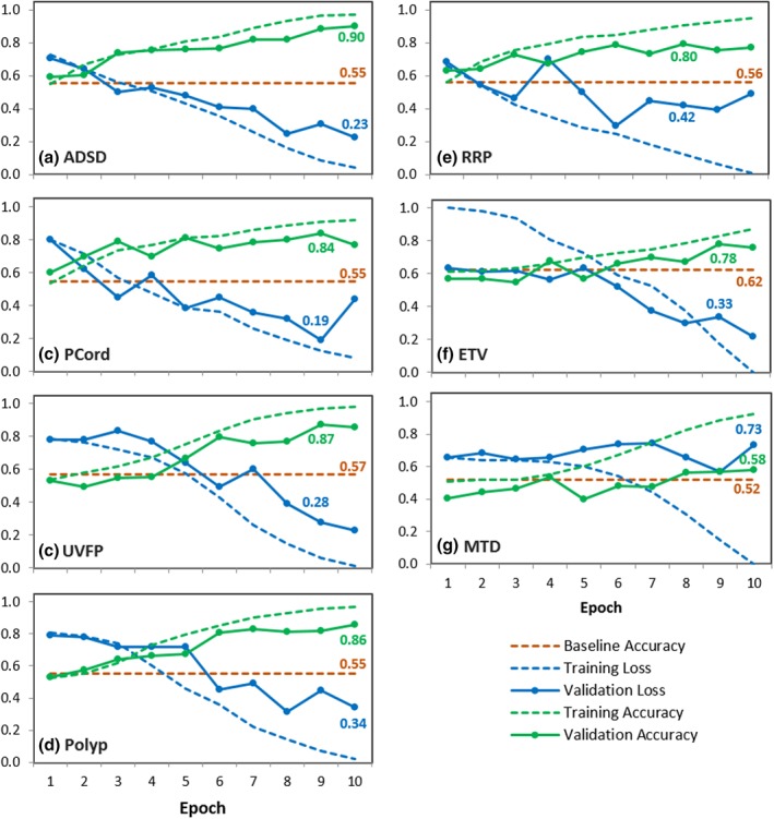
Average results of all folds obtained from 10‐fold cross validation for the binary classification of (a) adductor spasmodic dysphonia, (b) polypoid corditis or Reinke's edema, (c) unilateral vocal fold paralysis, (d) vocal fold polyp, (e) recurrent respiratory papillomatosis, (f) essential tremor of voice, and (g) muscle tension dysphonia. Baseline accuracies, as well as the accuracy and loss results from the highest performing epochs are labeled for each model.

Figure 6.

Accuracy and loss results for the best fold for (a) muscle tension dysphonia and (b) essential tremor of voice. Baseline accuracies, as well as the accuracy and loss results from the highest performing epochs are labeled for each model.

The difference between the accuracy and loss values from the training data (dashed line) and the validation data (solid line) is a qualitative measure of overfitting. The similar training and validation curves in the ADSD, PCord, and UVFP averaged models (Fig. 5a‐c) indicate minimal overfitting. Although overfitting was prominent in the Polyp, RRP, ETV, and MTD averaged models (Fig. 5d‐g), individual folds within these models demonstrated an absence of overfitting as shown in Figure 6a‐b.

DISCUSSION

Current Findings

In this proof‐of‐concept study, we investigated the utility of employing image analysis with deep learning to differentiate between normal and disordered voices using spectrograms. The averaged models achieved substantially higher accuracy in the validation set compared to the naïve algorithm for classifying normal vs adductor spasmodic dysphonia (90%), polypoid corditis (84%), unilateral vocal fold paralysis (87%), vocal fold polyp (86%), and recurrent respiratory papillomatosis (80%) voice samples, as shown in Figure 5a‐e. While the average models for muscle tension dysphonia and essential tremor of voice were comparably less robust (Fig. 5f‐g), results are consistent with other studies that employ artificial intelligence models to differentiate normal vs dysphonic voices.5 Furthermore, within these diagnostic groups, spectrograms from individual speakers (ie, specific folds) were classified with accuracies greater than 90%, as shown in Figure 6. We hypothesize that the variability in results from individual folds stem from individual patients’ symptom severity, and subsequently, individuals with a more severe presentation of the voice disorder may be classified more accurately. These results are promising (despite the small dataset used for this study) and the accuracy of these models should improve with additional training data.

The cross‐validation models for all seven classification tasks demonstrated overfitting after the tenth epoch of training, despite the dropout layers added for regularization. Overfitting occurs when the model adapts too closely to the idiosyncrasies of the training set and is unable to generalize to new data (ie, the validation set). This type of modeling error is common in highly complex models and is exacerbated by small sample sizes. The training set augmentation technique employed in this study both decreased overfitting and increased the accuracy of these models by a minimum of 5% (mean of 8%, data not shown). While spectrograms are sensitive to orientation for correct interpretation, other augmentation techniques to be explored include time scaling, time shifting, and pitch shifting.16 Ultimately, increasing the sample size would reasonably reduce overfitting and improve the generalizability of the model without the use of any image augmentation.

Challenges and Future Directions

The primary limiting factor in our proof‐of‐concept study is a lack of sufficient data. The current results are based on data from 80 individuals with a total sample size of 451 spectrograms. Each classification task, however, included data from the normal group and only one disordered group. The mean sample size for each classification task was therefore only 103, 3‐second spectrograms (Table 1).

While initial results for these seven voice disorders are promising, a robust dataset that represents the full range of severities across a broad range of voice disorders, as well as the wide variability among vocally healthy speakers, is critical to improve the models. Current efforts are underway to gather thousands of new and existing voice samples from patients and vocally healthy participants. However, the need for big data necessitates data collection protocols that minimize salient variabilities in recording conditions, and similarly requires models that are robust against these inconsistencies. Recordings must also be actively curated to maintain the fidelity of the training set, which is time‐consuming and expensive.

Although these challenges are non‐trivial, the potential clinical import of a robust, artificial intelligence‐driven, acoustic analysis tool is worth the effort. Such a tool has the potential to improve diagnostic accuracy and reliability and provide a standardized metric for interpretation within and between clinical institutions.

CONCLUSION

In this paper we applied image classification techniques with deep learning to classify spectrograms into normal vs disordered voices. Despite the small size of the available dataset, satisfactory results were obtained for the adductor spasmodic dysphonia, polypoid corditis, unilateral vocal fold paralysis, vocal fold polyp, and recurrent respiratory papillomatosis diagnostic groups, with accuracy in the validation set substantially higher than the baseline accuracy of the naïve algorithm. These preliminary results support further study of deep neural networks for clinical detection and diagnosis of human voice disorders.

BIBLIOGRAPHY

- 1. Kreiman J, Gerratt BR, Precoda K. Listener experience and perception of voice quality. J Speech Lang Hear Res 1990;33(1):103–115. [DOI] [PubMed] [Google Scholar]
- 2. Lieberman P. Some acoustic measures of the fundamental periodicity of normal and pathologic larynges. J Acoust Soc Am 1963;35(3):344–353. [Google Scholar]
- 3. Sáenz‐Lechón N, Godino‐Llorente JI, Osma‐Ruiz V, Gómez‐Vilda P. Methodological issues in the development of automatic systems for voice pathology detection. Biomed Signal Process Control 2006;1(2):120–128. [Google Scholar]
- 4. Hadjitodorov S, Mitev P. A computer system for acoustic analysis of pathological voices and laryngeal diseases screening. Med Eng Phys 2002;24(6):419–429. [DOI] [PubMed] [Google Scholar]
- 5. Schönweiler R, Hess M, Wübbelt P, Ptok M. Novel approach to acoustical voice analysis using artificial neural networks. J Assoc Res Otolaryngol 2000;1(4):270–282. [DOI] [PubMed] [Google Scholar]
- 6. Linder R, Albers AE, Hess M, Pöppl SJ, Schönweiler R. Artificial neural network‐based classification to screen for dysphonia using psychoacoustic scaling of acoustic voice features. J Voice 2008;22(2):155–163. [DOI] [PubMed] [Google Scholar]
- 7. Godino‐Llorente JI, Gomez‐Vilda P. Automatic detection of voice impairments by means of short‐term cepstral parameters and neural network based detectors. IEEE Trans Biomed Eng 2004;51(2):380–384. [DOI] [PubMed] [Google Scholar]
- 8. Lee H, Pham P, Largman Y, Ng AY. Unsupervised feature learning for audio classification using convolutional deep belief networks In: Bengio Y, Schuurmans D, Lafferty JD, Williams CKI, Culotta A, eds. Advances in Neural Information Processing Systems. Curran; 2009:1096–1104. [Google Scholar]
- 9. Deng L, Li J, Huang J‐T, et al. Recent advances in deep learning for speech research at Microsoft. 2013. IEEE Int Conf Acoust Speech Signal Process 2013:8604–8608. [Google Scholar]
- 10. Dheeba J, Singh NA, Selvi ST. Computer‐aided detection of breast cancer on mammograms: a swarm intelligence optimized wavelet neural network approach. J Biomed Inform 2014;49:45–52. [DOI] [PubMed] [Google Scholar]
- 11. Esteva A, Kuprel B, Novoa RA, et al. Dermatologist‐level classification of skin cancer with deep neural networks. Nature 2017;542(7639):115–118. [DOI] [PMC free article] [PubMed] [Google Scholar]
- 12. Fairbanks G. Voice and Articulation Drillbook: 2nd ed. New York: Harper & Row; 1960. [Google Scholar]
- 13. Sprengel E, Jaggi M, Kilcher Y, Hofmann T. Audio based bird species identification using deep learning techniques. LifeCLEF 2016:547–559. [Google Scholar]
- 14. Chollet F. Deep Learning with Python. Greenwich, CT: Manning Publications; 2017. [Google Scholar]
- 15. Sejdić E, Djurović I, Jiang J. Time–frequency feature representation using energy concentration: an overview of recent advances. Digit Signal Process 2009;19(1):153–183. [Google Scholar]
- 16. Salamon J, Bello JP. Deep Convolutional neural networks and data augmentation for environmental sound classification. IEEE Signal Process Lett 2017;24(3):279–283. [Google Scholar]