Robust optimization for intensity‐modulated proton therapy with soft spot sensitivity regularization

Abstract

Purpose

Proton dose distribution is sensitive to uncertainties in range estimation and patient positioning. Currently, the proton robustness is managed by worst‐case scenario optimization methods, which are computationally inefficient. To overcome these challenges, we develop a novel intensity‐modulated proton therapy (IMPT) optimization method that integrates dose fidelity with a sensitivity term that describes dose perturbation as the result of range and positioning uncertainties.

Methods

In the integrated optimization framework, the optimization cost function is formulated to include two terms: a dose fidelity term and a robustness term penalizing the inner product of the scanning spot sensitivity and intensity. The sensitivity of an IMPT scanning spot to perturbations is defined as the dose distribution variation induced by range and positioning errors. To evaluate the sensitivity, the spatial gradient of the dose distribution of a specific spot is first calculated. The spot sensitivity is then determined by the total absolute value of the directional gradients of all affected voxels. The fast iterative shrinkage‐thresholding algorithm is used to solve the optimization problem. This method was tested on three skull base tumor (SBT) patients and three bilateral head‐and‐neck (H&N) patients. The proposed sensitivity‐regularized method (SenR) was implemented on both clinic target volume (CTV) and planning target volume (PTV). They were compared with conventional PTV‐based optimization method (Conv) and CTV‐based voxel‐wise worst‐case scenario optimization approach (WC).

Results

Under the nominal condition without uncertainties, the three methods achieved similar CTV dose coverage, while the CTV‐based SenR approach better spared organs at risks (OARs) compared with the WC approach, with an average reduction of [Dmean, Dmax] of [4.72, 3.38]  GyRBE for the SBT cases and [2.54, 3.33] GyRBE for the H&N cases. The OAR sparing of the PTV‐based SenR method was comparable with the WC method. The WC method, and SenR approaches all improved the plan robustness from the conventional PTV‐based method. On average, under range uncertainties, the lowest [D95%, V95%, V100%] of CTV were increased from [93.75%, 88.47%, 47.37%] in the Conv method, to [99.28%, 99.51%, 86.64%] in the WC method, [97.71%, 97.85%, 81.65%] in the SenR‐CTV method and [98.77%, 99.30%, 85.12%] in the SenR‐PTV method, respectively. Under setup uncertainties, the average lowest [D95%, V95%, V100%] of CTV were increased from [95.35%, 94.92%, 65.12%] in the Conv method, to [99.43%, 99.63%, 87.12%] in the WC method, [96.97%, 97.13%, 77.86%] in the SenR‐CTV method, and [98.21%, 98.34%, 83.88%] in the SenR‐PTV method, respectively. The runtime of the SenR optimization is eight times shorter than that of the voxel‐wise worst‐case method.

Conclusion

We developed a novel computationally efficient robust optimization method for IMPT. The robustness is calculated as the spot sensitivity to both range and shift perturbations. The dose fidelity term is then regularized by the sensitivity term for the flexibility and trade‐off between the dosimetry and the robustness. In the stress test, SenR is more resilient to unexpected uncertainties. These advantages in combination with its fast computation time make it a viable candidate for clinical IMPT planning.

1. Introduction

Multifield optimized intensity‐modulated proton therapy (MFO‐IMPT, short for IMPT in this paper) is an effective technique to deliver highly conformal dose to the target volume while achieving superior organs at risk (OARs) sparing. However, due to the sharp drop‐off at the proton Bragg peak¹ and the beam‐by‐beam dose heterogeneity in the MFO plans,² IMPT is more susceptible to patient positioning errors or proton beam range uncertainties.^{3, 4, 5, 6, 7, 8} If the setup and range uncertainties are unaccounted for, dose to the tumor or OARs can substantially differ from what is indicated in the treatment plan. Different from x‐ray treatment planning, the proton dose deviation can happen not only at the target boundaries but also inside the target, making traditional planning target volume (PTV)‐based optimization, which expands the clinic target volume (CTV) by a safety margin, ineffective for IMPT.⁹

Several approaches have been developed to address this problem. Rather than a constant margin, a beam‐specific PTV¹⁰ is introduced, to vary the margin based on the field and tissue property for passive scattering and single field uniform dose IMPT (SFUD‐IMPT). Nevertheless, this approach is inapplicable to MFO‐IMPT. A theoretically appealing way to account for uncertainties was reported to calculate the dose distribution under random perturbations and optimizes the expectation value of the objective function.^{7, 8} However, due to the large statistical sampling required, the probabilistic approach is too slow for practical use. An alternative probabilistic approach is analytical probabilistic modeling (APM),^{11, 12} which uses a Gaussian pencil beam dose calculation algorithm to generate closed‐form propagation of probability distributions to quantify uncertainty input for probabilistic optimization. APM is faster because scenario‐sampling is not required, but estimation of the covariance requires nontrivial amount of computational resource that increases the optimization time. Furthermore, APM is incompatible with nonmodel‐based pencil beam dose calculation, for example, Monte Carlo, that is particularly important in handling the lateral dose profile and tissue heterogeneity in proton treatment planning. Coverage optimized planning¹³ is also a probabilistic treatment planning‐based method, which uses dose coverage histogram criteria to replace PTV margin and improves target dose coverage against geometric uncertainties, for example, setup error. Nonetheless, range uncertainty is not considered in this method. Alternatively, Pflugfelder et al.¹⁴ proposed to use a heterogeneity number to quantify lateral tissue heterogeneity of single scanning spot, and incorporated it in the inverse optimization to suppress the spots with a high heterogeneity number. This empirical method only considers the effect of tissue lateral heterogeneity to setup uncertainty without accounting for the range uncertainties. This method later pivoted towards beam angle selection,^{15, 16} a separate problem from our current focus of robust scanning spot intensity optimization.

Presently, a class of methods referred as “worst‐case robust optimization” is more commonly used to handle setup and range uncertainties.^{2, 7, 17, 18, 19, 20, 21, 22, 23, 24, 25, 26} Instead of considering all possible variations, the worst‐case method penalizes the maximal dose deviation for the estimated worst positioning and range estimation errors, to ensure acceptable dose distribution in these cases. In practice, the worst‐case approach has reduced plan sensitivity to uncertainties, but on the other hand increased computational cost. Furthermore, the worst cases use generic estimation that may not be applicable to all cases. The actual patient anatomical and range uncertainties may still exceed the estimation, causing unexpected dosimetric deviations.

In this work, we aim to overcome these limitations and develop a novel mathematical framework to exploit the intricate balance between the proton scanning spot distribution, robustness, and dose conformality. The plan robustness is incorporated as a sensitivity term in IMPT optimization, which minimizes the dose deviation from ideal dose distribution and penalizes the combination of scanning spots with high sensitivity.

2. Materials and methods

The sensitivity‐based robust optimization problem is formulated with a dose fidelity term and a robustness regularization term. The details are described as follows.

2.A. Sensitivity analysis

The dose calculation matrix, or the dose influence matrix, denoted as A, contains the vectorized dose information delivered to the patient volume from scanning spots of unit intensities. In this study, the position of individual scanning spots is denoted by the location of the Bragg peak in the patient volume. The sensitivity of a spot is determined by the magnitude of dose distribution for the perturbation due to patient position and range variations. To make the plan more resilient to changes, the spot position combinations with high sensitivity are penalized. Spatial dose gradient, which is used as a surrogate of spot sensitivity, is mathematically described as follows.

As shown in Fig. 1, a laboratory coordinate ( e ₁ , e ₂ , e ₃ ) is firstly created with its origin at the isocenter. b _i is the vector representing the direction of ith beam, pointing from the source to the isocenter. Because of the typically long proton source‐to‐axis distance, the scanning pencil beams from the same beam angle are nearly parallel. For simplicity, all the scanning spots belonging to the same beam share one b _i vector. p _j is a vector representing the spatial position of scanning spot j, which points from the isocenter to the Bragg peak position of spot j in the patient. Then let a _j ( b _i , p _j ) be the jth column in matrix A, which represents the dose from the jth scanning spot in the ith beam.

Figure 1.

Diagram showing the coordinates and the vectors used in spot sensitivity calculation. The beam divergence due to spot lateral distance to the isocenter is exaggerated for illustration purposes. The actual proton system source‐to‐axis distance is substantially greater than the target size and the individual pencil beams in the same beam direction are nearly parallel. [Color figure can be viewed at wileyonlinelibrary.com]

The gradient of a _j ( b _i , p _j ) with respect to p _j is written as:

$${\mathrm{\nabla }}_{{\mathit{p}}_j}{\mathit{a}}_j({\mathit{b}}_i,{\mathit{p}}_j).$$

If there are m elements (meaning m voxels in the patient volume) in the vector a _j ( b _i , p _j ), then ${\mathrm{\nabla }}_{{\mathit{p}}_j}{\mathit{a}}_j({\mathit{b}}_i,{\mathit{p}}_j)$ is a 3 × m matrix, with each row representing a directional derivative.

A beam's eye view is created for each beam, as shown in Fig. 1, denoted as ( b _i , u _i , v _i ), while ( u _i , v _i ) is the plane perpendicular to b _i . Therefore, the gradient along the beam direction is:

$$⟨{\mathit{b}}_i,{\mathrm{\nabla }}_{{\mathit{p}}_j}{\mathit{a}}_j({\mathit{b}}_i,{\mathit{p}}_j)⟩,$$

and the gradients orthogonal to beam direction are:

$$⟨{\mathit{u}}_i,{\mathrm{\nabla }}_{{\mathit{p}}_j}{\mathit{a}}_j({\mathit{b}}_i,{\mathit{p}}_j)⟩,$$

$$⟨{\mathit{v}}_i,{\mathrm{\nabla }}_{{\mathit{p}}_j}{\mathit{a}}_j({\mathit{b}}_i,{\mathit{p}}_j)⟩.$$

The 〈·〉 operator stands for vector inner product. Each of the directional gradients is a 1 × m vector. The absolute value of each component in the directional gradients, which measures the magnitude of dose variation between neighborhoods spots, is more useful in this framework. The definition of directional gradient based on the variation between neighboring spots can be intuitively understood as follows. If the beam directions are nearly parallel to the interface of different densities, which means high lateral tissue heterogeneity, neighboring spots will then contribute dose to very different voxels, resulting in a higher gradient and sensitivity value. Our algorithm will then penalize more heavily on these spots that are affected by higher lateral tissue heterogeneity to improve plan robustness. We use the notation | x | to mean the absolute value of each component of the vector x . The element‐wise absolute values of the three directional gradients are written as:

$$\left|⟨b_i,{\mathrm{\nabla }}_{p_j}{a}_j(b_i,p_j)⟩\right|,\left|⟨u_i,{\mathrm{\nabla }}_{p_j}{a}_j(b_i,p_j)⟩\right|,\text{and}\left|⟨v_i,{\mathrm{\nabla }}_{p_j}{a}_j(b_i,p_j)⟩\right|.$$

Applying this operation to every column of the A matrix (j = 1, …, n, i = 1, …, r, where n is the number of scanning spots and r is the number of beams), we acquire three sensitivity matrices: ΔA _b , ΔA _u , and ΔA _v , which are formulated as:

$$\begin{array}{cc}\hfill \mathrm{\Delta }{A}_{\mathit{b}}& =\left[\left|⟨{\mathit{b}}_1,{\mathrm{\nabla }}_{{\mathit{p}}_1}{\mathit{a}}_1{({\mathit{b}}_1,{\mathit{p}}_1)⟩}^T\right|,\dots ,\left|⟨{\mathit{b}}_r,{\mathrm{\nabla }}_{{\mathit{p}}_n}{\mathit{a}}_n{({\mathit{b}}_r,{\mathit{p}}_n)⟩}^T\right|\right],\hfill \\ \hfill \mathrm{\Delta }{A}_{\mathit{u}}& =\left[\left|⟨{\mathit{u}}_1,{\mathrm{\nabla }}_{{\mathit{p}}_1}{\mathit{a}}_1{\left({\mathit{b}}_1,{\mathit{p}}_1\right)⟩}^T\right|,\dots ,\left|{\mathit{u}}_r,{\mathrm{\nabla }}_{{\mathit{p}}_n}{\mathit{a}}_n{\left({\mathit{b}}_r,{\mathit{p}}_n\right)⟩}^T\right|\right],\hfill \\ \hfill \mathrm{\Delta }{A}_{\mathit{v}}& =\left[\left|{⟨{\mathit{v}}_1,{\mathrm{\nabla }}_{{\mathit{p}}_1}{\mathit{a}}_1\left({\mathit{b}}_1,{\mathit{p}}_1\right)⟩}^T\right|,\dots ,\left|{⟨{\mathit{v}}_r,{\mathrm{\nabla }}_{{\mathit{p}}_n}{\mathit{a}}_n\left({\mathit{b}}_r,{\mathit{p}}_n\right)⟩}^T\right|\right]\hfill \end{array}.$$

The three matrices have a size of $m\times n$. ΔA _b evaluates the dose sensitivity level at each element from each scanning spot along longitudinal direction (beam direction), and ΔA _u and ΔA _v both evaluate the lateral sensitivity (perpendicular to beam direction). In this study, only ΔA _b and ΔA _u are used for optimization in the following sections.

2.B. Problem formation

As mentioned before, the spots are penalized based on their sensitivities. With the formation of sensitivity matrices along the beam direction and perpendicular to the beam direction, an intuitive approach is to penalize the L2,2‐norm of $\mathrm{\Delta }{A}_k\mathit{x},\left(k\in \left\{\mathit{b},\mathit{u}\right\}\right)$, which is formulated as:

$$\begin{array}{cc}& \underset{\mathit{x}}{\text{minimize}}\mathrm{\Gamma }(A\mathit{x})+{\lambda }_{\mathit{b}}{∥\mathrm{\Delta }{A}_{\mathit{b}}\mathit{x}∥}_2^2+{\lambda }_u{∥\mathrm{\Delta }{A}_u\mathit{x}∥}_2^2,\hfill \\ & \text{subject to}\mathit{x}\ge 0,\hfill \end{array}$$ (1)

where x is the optimization variable representing the scanning spot intensities, Γ(Ax ) is the dose fidelity term penalizing the dose deviation from ideal dose distribution, and λ _b and λ _u are the sensitivity regularization parameters. A common choice for Γ(Ax ) is the quadratic loss function, which is written as:

$$\mathrm{\Gamma }(A\mathit{x})=\sum _{q\in \mathcal{T}}{w}_q\Vert {(l_q-A_q\mathit{x})}_{+}{\Vert }_2^2+\sum _{q\in \mathcal{O}}{w}_q{\Vert {(A_q\mathit{x}-d_q)}_{+}\Vert }_2^2,$$ (2)

where $\mathcal{T}$ is the dose‐promoting structure set which usually includes all the target volumes, and $\mathcal{O}$ is the dose‐limiting structure set which includes the OARs as well as the target volumes if the hot spots need to be suppressed. A _q is the dose calculation matrix of structure q. l _q is the prescription dose to qth target volume, d _q is the prescribed maximal allowed dose to mth structure, and w _q is the structure‐specific weighting parameter.

However, the matrix ΔA _k (k ∈ { b , u }) has the same size as the matrix A, which makes it time and memory expensive to solve the problem (1). To improve the computational efficiency, as suggested by Ungun et al.²⁷, an L1‐norm is used as a surrogate of the L2, 2‐norm and column clustering on the sensitivity matrix is performed to reduce the problem size. The problem is then formulated as:

$$\begin{array}{cc}& \underset{\mathit{x}}{\text{minimize}}\mathrm{\Gamma }(A\mathit{x})+\sum _{k\in \{\mathit{b},u\}}{\lambda }_k{\Vert \mathrm{\Delta }{A}_k\mathit{x}\Vert }_1,\hfill \\ & \text{subject to}\mathit{x}\ge 0,\hfill \end{array}$$ (3)

The sum of the absolute values of the row vectors of ΔA _b and ΔA _u is calculated and the corresponding transpose is denoted as s _b and s _u , respectively, which is called the sensitivity vector. Then, the sensitivity‐regularized robust optimization problem is written as:

$$\begin{array}{cc}& \underset{\mathit{x}}{\text{minimize}}\mathrm{\Gamma }(A\mathit{x})+\sum _{k\in \{\mathit{b},u\}}{\lambda }_k{\mathit{s}}_k^T\mathit{x},\hfill \\ & \text{subject to}\mathit{x}\ge 0,\hfill \end{array}$$ (4)

The initial large‐scale matrix and vector multiplication in problem (1) is reduced to a vector inner product, which is computationally inexpensive. Moreover, problem (4) is a convex problem and can be solved by FISTA, an accelerated proximal gradient method known as the fast iterative shrinkage‐thresholding algorithm.²⁸ The details of solving the problem (4) using FISTA are shown in Appendix A.

2.C. Evaluations

This proposed sensitivity‐regularized (SenR) method was tested on three patients with skull base tumor (SBT) and three bilateral head‐and‐neck (H&N) patients, and was compared against conventional PTV‐based optimization method (Conv) and voxel‐wise worst‐case optimization method (WC).^{2, 7, 19, 21} The voxel‐wise worst‐case optimization considered nine scenarios, including one nominal scenario and eight worst‐case scenarios. The eight worst‐case scenarios consist of (a) six setup uncertainty scenarios, by shifting the beam isocenter by ±3 mm along anteroposterior, superior‐inferior, and mediolateral directions; (b) two range uncertainties scenarios, by scaling the computed tomography (CT) number by ±3%. The same quadratic cost function as Eq. (2) is used for worst‐case method and it is solved by a first‐order primal‐dual algorithm known as Chambolle–Pock algorithm.²⁹ The details of solving this problem in our study are shown in Appendix B.

For every patient, the same beam arrangement, scanning spot population scheme, and dose calculation engine were used for the three methods. The dose calculation for all scanning spots covering the CTV and a 5‐mm margin was performed by matRad,^{30, 31} a MATLAB‐based three‐dimensional (3D) treatment planning toolkit. The dose calculation resolution was 2.5× 2.5× 2.5 mm. The target volume for worst‐case approach was chosen to be CTV, and the conventional method was planned based on the PTV, which was a 3‐mm isotropic expansion of the CTV. Our sensitivity‐regularized method was applied to both CTV and PTV to investigate the impact of margin in the new optimization framework. The prescription dose, target volume and the beam arrangement are shown in Table 1.

Table 1.

Prescription doses, CTV volumes, and the beam angles (gantry, couch)

Case		Prescription dose (GyRBE)	CTV volume (cc)	Beam angle
SBT #1	CTV63	63	86.07	(270, 0) (90, 0) (180, 0) (60, 275)
	CTV74	74	26.42
SBT #2		70	36.8
SBT #3		56	33.7
H&N #1	CTV54	54	141.29	(0,0) (160,0) (200,0)
	CTV60	60	160.89
	CTV63	63	68.00
H&N #2	CTV54	54	108.00
	CTV60	60	127.26
H&N #3	CTV54	54	110.38
	CTV60	60	98.94
	CTV63	63	10.23

The nominal dose distribution and robustness against range uncertainties and setup uncertainties were both evaluated. Under the nominal situation, The CTV homogeneity, D95%, D98%, and maximum dose were evaluated. CTV homogeneity is defined as D95%/D5%. The maximum dose is defined as the dose to 2% of the structure volume, D2%, following the recommendation by IRCU‐83.³² The mean and maximum doses for OARs were also evaluated. The robustness was evaluated by the same nine scenarios used for worst‐case optimization. The dose volume histogram (DVH) band plot, as well as the worst dose metrics occurred among uncertainties scenarios, was used for analysis. In addition to the 3% range uncertainty, a stress test was performed on the normalized CTV volume covered by the 100% prescription dose for the range estimation error varying from 0.5% to 4.0%, with 0.5% interval.

In order to assess the applicability of L1‐norm and column clustering, we compared the nominal dose and robustness of plans for an SBT and a H&N patient using function (1), which is sensitivity matrix based, and function (4), which is sensitivity vector based.

Because matRad uses a pencil beam algorithm for dose calculation, which can cause inaccurate sensitivity matrix assessment in heterogeneous tissue, it was benchmarked against goPMC,^{33, 34, 35} a graphics‐processing unit (GPU) OpenCL‐based Monte Carlo (MC) proton dose calculation engine for a selected beam in an SBT case. The same proton phase space data were used for matRad and goPMC. 1 × 10⁶ primary proton particles per pencil beam were simulated in goPMC. The differences in sensitivity vectors from the two engines were evaluated.

3. Results

Using an i7 6‐core CPU desktop, the time spent on dose calculation, sensitivity vector evaluation, and optimization of each method are listed in Table 2. Parallel computing toolbox in Matlab was used to accelerate the worst‐case dose calculation and sensitivity evaluation. The preparation time before optimization for the WC method and the SenR method was comparable. During optimization, the SenR method using PTV as target volume (SenR‐PTV) was as efficient as the Conv method, and it was on average 22 times faster than the WC method. And the SenR plans using CTV as target volume (SenR‐CTV) were faster than the SenR‐PTV plans due to fewer voxels to consider during optimization. One thing to note is that the computational time comparison is based on the solvers developed in our group, and the actual time of voxel‐wise worst‐case method will be different in commercial treatment planning system.

Table 2.

Computational time comparison of the four plans of each patient

Case	Pre‐optimization time (s)			Optimization runtime (s)
	Nominal dose calculation	Worst‐case dose calculation	Sensitivity calculation	Conv	WC	SenR‐PTV	SenR‐CTV
SBT #1	41.87	106.3	129.8	75.5	2296.5	74.1	66.7
SBT #2	29.95	66.8	55.3	73.1	1070.6	73.4	73.0
SBT #3	28.22	75.5	44.7	76.0	909.5	75.1	59.9
H&N #1	210.01	638.1	408.6	129.7	2211.6	129.4	93.8
H&N #2	208.73	649.2	346.6	114.7	2477.0	105.4	80.9
H&N #3	174.32	546.6	408.6	121.5	3269.0	133.0	103.4

A sensitivity color map is shown in Fig. 2, which indicates the intensity of each element in the sensitivity vector and its spatial position, for a right lateral beam in the SBT #2 patient case. The sensitivity values in both longitudinal and lateral directions varied with the spot spatial positions. The scanning spots located in the region with higher tissue heterogeneity, like ones near the nasal cavity shown in the CT image, tended to be more sensitive to perturbation. Figure 2 compares the sensitivity results calculated using matRad and goPMC. The sensitivity distributions from the two dose calculation engines visually agreed with each other. The range of sensitivity values from matRad was smaller than that from goPMC. Quantitatively, the average difference of sensitivities between matRad and goPMC was 1.45% and 6.61% in the lateral and the longitudinal directions, respectively.

Figure 2.

The Bragg peak position of the scanning spots from a right lateral beam, on a selected transverse plane of the SBT #2 patient, and the intensities of sensitivities of these scanning spots shown in color map. The result from matRad is shown on the left and the result from goPMC on the right. The sensitivity perpendicular (lateral) to the beam direction is in the top row and the sensitivity along beam direction (longitudinal) is in the bottom row. The red contour in the CT image is CTV. [Color figure can be viewed at wileyonlinelibrary.com]

3.A. Nominal dose comparison

Figure 3 shows the nominal DVH comparison among the WC plans, SenR‐CTV plans, and SenR‐PTV plans for the SBT #1 patient and H&N #2 patient. Figure 4 compares the nominal CTV statistics of each patient using different optimization methods. Several OARs are selected for the SBT and H&N sites, respectively, and the differences in their mean and maximum doses between the SenR plans and the WC plans are presented in Tables 3 and 4. Without uncertainties, the Conv, WC, SenR‐PTV, and SenR‐CTV methods achieved similar CTV dose coverage.

Figure 3.

Comparison of nominal DVHs for patients skull base tumor #1 and H&N #1 of the WC method (solid), SenR‐CTV method (dotted), and SenR‐PTV method (dashed). [Color figure can be viewed at wileyonlinelibrary.com]

Figure 4.

Comparison of clinic target volume homogeneity, D98%, D95%, and Dmax for skull base tumor patients (top row) and H&N patients (bottom row) under nominal situation. [Color figure can be viewed at wileyonlinelibrary.com]

Table 3.

Organs at risk mean dose and max dose reduction of the SenR plans from the WC plans, for the skull base tumor (SBT) cases under nominal situation

SBT case	SenR‐CTV — WC (GyRBE)						SenR‐PTV — WC (GyRBE)
	Dmean			Dmax			Dmean			Dmax
	#1	#2	#3	#1	#2	#3	#1	#2	#3	#1	#2	#3
Left optical nerve	−8.38	−4.34	−4.82	−3.50	−2.93	−1.06	−2.31	−4.95	+1.10	−1.50	−2.13	−0.65
Right optical nerve	−4.51	−0.96	−9.87	+0.53	−4.20	−2.68	−0.71	−0.71	−2.04	+1.34	−1.00	+2.00
Chiasm	−1.21	−8.92	−1.57	0.00	−4.20	−0.29	+2.06	−3.29	+0.54	−0.10	−8.00	−0.86
Brainstem	−6.78	−3.60	−1.29	−1.94	−7.58	−3.65	−6.23	−2.54	−1.16	−2.36	−0.92	−2.73
Left cochlea	−20.15	−3.45	0.00	−18.0	−1.00	0.00	−13.11	+6.23	0.00	−9.00	+11.40	0.00
Right cochlea	−4.44	−0.63	0.00	−9.61	−0.80	0.00	−7.00	−2.01	0.00	−11.20	−1.44	0.00

Table 4.

Organs at risks mean dose and max dose reduction of the SenR plans from the WC plans, for the H&N cases under nominal situation

H&N case	SenR‐CTV – WC (GyRBE)						SenR‐PTV – WC (GyRBE)
	Dmean			Dmax			Dmean			Dmax
	#1	#2	#3	#1	#2	#3	#1	#2	#3	#1	#2	#3
Brainstem	−0.45	−1.09	−0.21	−2.00	−4.75	−2.56	−0.08	−1.22	−0.13	−1.00	−8.27	−1.60
Constrictors	−3.50	−3.17	−2.87	−10.60	−3.13	−1.24	−1.01	+0.50	+3.25	+3.70	+2.42	+3.21
Right submandibular gland	+3.38	−15.98	+1.16	+0.04	−3.65	−1.15	+2.98	−0.58	−10.01	+0.36	−1.22	−1.45
Larynx	−6.31	−1.88	−2.84	−11.68	−4.90	−7.49	−3.42	−0.78	−2.73	−4.07	−1.04	−6.29
Left parotid	−3.80	−9.47	−1.15	−0.48	−2.10	−0.34	−0.76	−2.06	+1.58	−0.74	−1.07	+1.71
Right parotid	−0.80	−0.66	−0.07	−3.08	−0.22	−0.69	+0.21	−0.83	+1.08	+3.40	−1.76	+3.89
Spinal cord	−1.31	−1.08	−1.27	−3.29	−2.30	−4.29	−1.07	−0.68	−1.32	−1.50	−0.10	−5.39

The SenR‐CTV plans had better OAR sparing compared with the WC plans. For example, in the SBT #1 patient, SenR‐CTV reduced the mean dose and max dose of the left cochlea by 20.15 GyRBE and 18 GyRBE from WC, and the dose sparing of other OARs were also improved except the max dose to the right optical nerve. In the H&N #1 patient, the doses to the parotids were also lower in SenR‐CTV plan compared with the WC plan. The average reduction of [Dmean, Dmax] of the SenR‐CTV plans from the WC plans were [4.72, 3.38] GyRBE for the SBT cases and [2.54, 3.33] GyRBE for the H&N cases.

The overall OAR sparing of SenR‐PTV was comparable with the WC. For example, in the three SBT cases, the mean and max brainstem doses were both reduced in SenR‐PTV relative to WC. SenR‐PTV plans also achieved lower Dmax to the left optical nerve and chiasm, but the Dmax to the left cochlea in the SBT #2 patient was greater due to an overlap with PTV. In the H&N case, a reduction of dose in the brainstem, larynx, and spinal cord was observed in the SenR‐PTV plans. The average reduction of [Dmean, Dmax] of the SenR‐PTV plans from the WC plans were of [2.00, 1.51] GyRBE for the SBT cases, and [0.81, 0.80] GyRBE for the H&N cases.

3.B. Robust analysis

The DVH bands of CTVs and selected OARs indicating the plan robustness with range and setup uncertainties for the SBT #1 and the H&N #2 patients are shown in Figs. 5 and 6, where the solid lines in each plot are the DVHs of the nominal case, and the bands bound the worst‐case distributions. A narrower band means greater resilience to uncertainties. Qualitatively, both the SenR approach and WC method improved the robustness of CTVs and OARs from conventional PTV‐based method for the two disease sites.

Figure 5.

DVH bands of the skull base tumor #1 patient including two range uncertainties (left column) and six setup uncertainties (right column). The first row is Conv plans, the second row is the WC plans, the third row is SenR‐CTV plans, and the last row is the SenR‐PTV plans. [Color figure can be viewed at wileyonlinelibrary.com]

Figure 6.

DVH bands of the H&N#2 patient including two range uncertainties (left column) and six setup uncertainties (right column). The first row is Conv plans, the second row is the WC plans, the third row is SenR‐CTV plans, and the last row is the SenR‐PTV plans. [Color figure can be viewed at wileyonlinelibrary.com]

With range uncertainties, similar or more compacted CTV bands were observed in the SenR‐PTV plans compared with the WC plans. The SenR‐CTV plans also resulted in narrow CTV bands, but there was a slightly larger underdosage region of CTV in these plans. The robustness against setup uncertainties was similarly improved by SenR‐PTV and SenR‐CTV.

In addition to better target volume robustness, a decrease in OAR sensitivity was observed in both the SenR‐PTV and SenR‐CTV plans. For example, the DVH bands of the optical nerves and optical chiasm in the SBT #1 patient, and the left parotid in the H&N#2 patient are narrower than that in Conv.

The lowest (worst) D95%, V95%, and V100% of each CTV with range uncertainties and setup uncertainties were also evaluated and plotted in Fig. 7. Compared with Conv plans, the D95%, V95%, and V100% were improved by SenR and WC. Overall SenR‐PTV and WC achieved better CTV dose metrics. On average, under range uncertainties, the lowest [D95%, V95%, V100%] of CTV were increased from [93.75%, 88.47%, 47.37%] in Conv, to [99.28%, 99.51%, 86.64%] in WC, [97.71%, 97.85%, 81.65%] in SenR‐CTV, and [98.77%, 99.30%, 85.12%] in SenR‐PTV, respectively. Under setup uncertainties, the average lowest [D95%, V95%, V100%] of CTV were increased from [95.35%, 94.92%, 65.12%] in Conv, to [99.43%, 99.63%, 87.12%] in WC, [96.97%, 97.13%, 77.86%] in SenR‐CTV, and [98.21%, 98.34%, 83.88%] in SenR‐PTV, respectively.

Figure 7.

The comparison of worst D95% (top row), worst V95% (second row), and worst V100% of the clinic target volumes as a percentage of prescription doses, for every patient. Situation with only range uncertainty is shown on the left and situation with only setup uncertainty is shown on the right. [Color figure can be viewed at wileyonlinelibrary.com]

Figure 8 shows the V100% stress test results, where the range estimation error was increased from 0% to 4%, which is 1.0% outside of the expected worst case. V100% degrades with increasing range estimation error but the SenR‐PTV method shows slower degradation and greater robustness than WC.

Figure 8.

The patient‐averaged worst V100% of the three methods, when range uncertainty varies from 0.0% to 4.0%. [Color figure can be viewed at wileyonlinelibrary.com]

The sensitivity regularization parameter tuning is demonstrated for a SenR‐PTV plan for H&N #2 by varying longitudinal direction (λ _b ) or lateral direction (λ _u ) parameter while fixing the structure weighting parameters. The worst D95% of the CTV60 as a function of λ _b and λ _u is shown in Fig. 9(a). Both the range robustness and setup robustness were improved with λ _b and λ _u increasing from 0 but the improvement plateaued or started to slowly reverse once the two parameters reached certain values. The presence of plateau region makes parameter selection repeatable. Understandably, λ _u and λ _b tunings have different effectiveness in improving plan range robustness and setup robustness. Figures 9(b) and 9(c) show that the increase in λ _u and λ _b leads to lower CTV heterogeneity and higher dose in some OARs. In our study we choose approximately the smallest value of λ _u and λ _b in the plateau region to improve robustness and maintain dosimetry. For example, in this H&N #2 patient, λ _u is chosen to be 1 and λ _b is chosen to be 1.2.

Figure 9.

(a) The worst D95% of CTV60 in the H&N #2 patient, and its relationship with the lateral sensitivity parameter λ _u and longitudinal sensitivity parameter λ _b . (b) The nominal DVH of the H&N #2 patient when λ _u  = 0 (solid line), 1 (dotted line), 4 (dashed line). (c) The nominal DVH of the H&N #2 patient when λ _b  = 0 (solid line), 1 (dotted line), 4 (dashed line). [Color figure can be viewed at wileyonlinelibrary.com]

To study if the collapse of the sensitivity matrix to vector in Eq. (3) and (4) would adversely impact the performance, the plans using sensitivity vector regularization (SenVec) and sensitivity matrix regularization (SenMat) were compared. The plans were created using PTV as target volume. For the two patient cases shown in Fig. 10, compared with the SenMat plans, the SenVec plans had similar or slightly better OAR sparing, and evidently superior robustness against either range error or setup error. As expected, the SenVec plans were two to three times faster to compute than the SenMat plans.

Figure 10.

Comparison of plans using sensitivity vector and sensitivity matrix regularization. The nominal DVH is shown in the first column, with SenMat in solid line and SenVec in dotted line. The latter two columns show the DVH band of the clinic target volumes under the range uncertainty (middle column) and setup uncertainty (last column). The skull base tumor #2 patient is shown in the top row and H&N #2 patient in the bottom row. [Color figure can be viewed at wileyonlinelibrary.com]

3.C. Spot‐level analysis

In order to better understand the mechanism of SenR method, an analysis on scanning spot level is demonstrated using the SBT #1 patient as example. The spot‐level dose difference between Conv method and SenR‐CTV method when undershooting (+3% range uncertainties) happens is shown in Fig. 11. In this analysis, a point of interest in the target, which is inside an underdosing area when undershooting, is found and the scanning spots located within a 2‐cm radius sphere of this cold spot are extracted. These scanning spots from four different beam directions are the main contributors to the dose of the point of interest. The total dose from these local scanning spots is shown in Fig. 11(a), with the first row being the transverse plane and the second row being the sagittal plane. From left to right, each column represents the Conv nominal, the Conv undershooting, SenR‐CTV nominal and SenR‐CTV undershooting conditions, respectively. The peak position of the dose distribution in the Conv (SenR) nominal plan is marked P _1· (P ₂ ), denoted as the crosshairs in the first (last) two columns of images in Fig. 11. P ₁ and P ₂ are used as the reference points when comparing the dose change when undershooting. For comparison, the isodose display is normalized to the P‐point dose of the corresponding nominal case without range error. When the range is overestimated, a 20% reduction in the P‐point dose is resulted in the Conv case. However, the high sensitivity combination is quantified in the new optimization framework and correctly penalized. As a result, to deliver dose to the same point of interest, a different combination of spots is selected. When the same undershooting happens, the P‐point dose only drops 5% in the SenR plan. A closer examination of the scanning spots distribution reveals why the SenR‐optimized combination is more resilient to the range estimation error. Different from the Conv approach that chooses spots that match their distal edges, in the SenR approach, spots are slightly mismatched. Spots from beam 1 and 4 contribute their proximal edges to P and the spot from beam 3 contributes its lateral edge. When the range is overestimated, the slightly undershot spots from beam 1 and 4 would retract while the contribution from beam 3 remains unchanged due to the smooth lateral dose profile. This combination is equally resilient to range underestimation due to the same reason that the dose to a given point is contributed by a mixture of distal, lateral, and proximal edges. The last two are not as sharp as the distal edge and are thus more resilient to range estimation error.

Figure 11.

Spot‐level analysis around a cold spot for the skull base tumor #1 patient when range undershooting. (a) The total dose from the local scanning spots within the 2‐cm radius sphere of the cold spot. The first row is the transverse plane and the second row is the sagittal plane. (b) The dose contribution of the local spots from each beam direction. From left to right, each column represents the Conv nominal condition, Conv undershooting condition, SenR‐CTV nominal condition and SenR‐CTV undershooting condition. [Color figure can be viewed at wileyonlinelibrary.com]

4. Discussion

Current proton treatment planning methods manage robustness by performing optimization on a finite number of hypothetical worst cases. A drawback for the existing worst‐case method is that it may be too conservative in certain cases, resulting in unacceptable dosimetric compromise³⁶ yet is inadequate for extreme case where the error exceeds expectation. The uncertainties are sparsely sampled in the worst‐case approach, which is unprepared for positioning and range errors different from these sparsely sampled cases. In comparison, in the SenR framework, robustness is included as a linear regularization term that not only softens the impact of robustness consideration but also allows flexible adjustment of the robustness to meet varying requirements. In the nominal cases where the uncertainties are low, the dosimetric quality is better preserved. Due to the differences, SenR method may particularly benefit cases where the uncertainties are difficult to accurately estimate, highly heterogeneous in the same cohort, or variable over the treatment course. Since the sensitivity is calculated as a gradient of the spot dose distribution, our method does not depend on a specific set of expected positioning or range uncertainties, which is needed in the worst‐case optimization. This difference lends the flexibility of trading off the robustness with dosimetry by adjusting the sensitivity term weighting without needing to estimate the uncertainties explicitly. This new robust optimization method is thus different from previous approaches of adjusting the worst‐case weights,¹⁹ using multicriteria optimization,²² and using the normalized dose interval volume constraints.³⁷

Another drawback of worst‐case methods is that they are computationally inefficient due to the time needed to optimize a significantly larger optimization problem for all scenarios. The runtime of the SenR optimization is 22 times shorter than that of the voxel‐wise worst‐case method excluding preoptimization calculation of the sensitivity matrix and worst‐case doses, and eight times shorter including preoptimization calculation, while achieving comparable robustness in the hypothetical worst cases.

In this study, the SenR method is implemented on both CTV and PTV. The SenR‐PTV method achieves comparable robustness towards the expected worst cases and OAR sparing as the WC method. Sen‐CTV attains superior OAR sparing with a slight compromise in the CTV robustness while avoiding the substantial degradation seen in the conventional PTV plans. The different target volumes offer additional flexibility in clinical practice for the trade‐off between OAR sparing and CTV coverage robustness. This is feasible also due to the demonstrated fast SenR planning speed. As an additional advantage, SenR is versatile and independent of the underlying proton dose calculation algorithms, of which, a model‐based method and a Monte Carlo method were used showing consistent results.

In the implemented SenR method, L2, 2‐norm and the sensitivity matrices were replaced by L1‐norm and the sensitivity vectors to improve the computational efficiency. Interestingly, the replacement is not only faster but also performs better for CTV robustness. A possible reason is due to the presence of spots with large sensitivity to uncertainties. L1‐norm is forgiving to these outliers and then more effectively regularizes most spots with moderate sensitivities.

The proposed method is particularly effective for targets in the heterogeneous environment where the sensitivity is captured in the perturbation term. The effectiveness of the regularized‐sensitivity is highly dependent on the beam and spot arrangement. As shown by the spot‐level analysis, instead of matching the distal edges, SenR tends to combine distal, proximal and lateral edges of spots for improved robustness. Figure 11 shows one of such possible robust combinations and the new optimization framework allows us to be efficient and globally find these combinations. The importance of combining spots for both plan robustness and conformality was discussed by Liu et al.^{2, 38} One of the main contributions here is to describe the intricate spot interdependence with a new mathematical model that can be efficiently solved.

The proposed method applies to scenarios where the same location is covered by multiple beams. However, field‐matching may happen when different parts of the CTV are treated by different beams. The proposed method may result in a mismatch in the gradients at the field‐matching lines that leads to cold and hot spots with position and range uncertainties. Further investigation is needed to understand and mitigate such dose heterogeneities.

The optimal spot combinations are likely beam orientation dependent. We have previously developed a beam orientation optimization framework for IMPT.³⁹ In this study, fixed beam orientations are used but both the SenR plan optimality and robustness can be conceivably improved by unifying the two optimization frameworks in future research.

5. Conclusions

We developed a novel computationally efficient robust optimization method for IMPT. The robustness is calculated as the spot sensitivity to both range and shift perturbations. The dose fidelity term is then regularized by the sensitivity term. The new SenR method offers the flexibility to balance between the dosimetry and the robustness. In the stress test, SenR is shown to be resilient to greater than expected uncertainties. These advantages in combination with its fast computation time make it a viable candidate for clinical IMPT planning.

Conflicts of interest

The authors have no relevant conflicts of interest to disclose.

Appendix A.

A.1.

To solve an optimization problem using FISTA, the problem needs to be formulated in the following form:

$$\underset{\mathit{x}}{\text{minimize}}f(\mathit{x})+g(\mathit{x}),$$ (A1)

where f is a smooth convex function, which is continuously differentiable with Lipschitz continuous gradient (∇f); g is a function which is possibly nonsmooth, but has a proximal operator that can be evaluated efficiently. The proximal operator with step size t > 0 for function g is defined by:

$${\text{prox}}_{\mathit{tg}}(x)=\underset{\mathit{y}}{\text{argmin}}g(\mathit{y})+\frac{1}{2t}{\Vert \mathit{y}-\mathit{x}\Vert }_2^2.$$ (A2)

Once the optimization problem is formulated as in Eq. (A1) and the conditions for f( x ) and g( x ) are satisfied, FISTA is relatively straightforward to implement as it only involves elementary matrix‐vector arithmetic operations and inexpensive proximal operator evaluations. FISTA with line search is used in this work, which follows the steps shown in Table AI

Table AI.

Pseudo code for FISTA with line search

In the problem (4), the objective function can be rewritten in the following format:

$$\begin{array}{cc}\hfill f(\mathit{x})& =\mathrm{\Gamma }(A\mathit{x})+\sum _{k\in \{\mathit{b},\mathit{u}\}}{\lambda }_k{\mathit{s}}_k^T\mathit{x}\hfill \\ \hfill g(\mathit{x})& =I_{\ge 0}(\mathit{x})\hfill \end{array},$$ (A3)

where I _≥0( x ) is an indicator function on non‐negative orthant, with its ith element equal to 0 if x _i  ≥ 0 and ∞ otherwise.

For the quadratic fidelity formulation, the gradient of f is given by:

$$\begin{array}{cc}\hfill \mathrm{\nabla }f(\mathit{x})=& A^{\mathrm{T}}\mathrm{\nabla }\mathrm{\Gamma }(A\mathit{x})\hfill \\ & +\sum _{k\in \{\mathit{b},\mathit{u}\}}{\lambda }_k{\mathit{s}}_k=\sum _{q\in \mathcal{T}}{w}_q{A}_q^{\mathit{T}}{(l_q-A_q\mathit{x})}_{+}\hfill \\ & +\sum _{q\in \mathcal{O}}{w}_q{A}_q^T{(A_q(\mathit{x})-d_q)}_{+}+\sum _{k\in \{\mathit{b},u\}}{\lambda }_k{\mathit{s}}_k,\hfill \end{array}$$ (A4)

The proximal operator of the function g is:

$${\text{prox}}_{\mathit{tg}}(\mathit{x})=P_{\ge 0}(\mathit{x}),$$ (A5)

where P _≥0( x ) is the projection of x onto non‐negative orthant.

Using these formulas for the gradient of the function f and the proximal operator of function g, the sensitivity regularization robust problem is readily solved using FISTA.

Appendix B.

B.1.

The set of considered error scenarios is denoted as $\mathcal{K}$, and the dose calculation matrix of each scenario is $A^k,k\in \mathcal{K}$. The voxel‐wise worst‐case optimization with quadratic cost function is formulated as the following problem:

$$\begin{array}{cc}& \underset{x}{\text{minimize}}\sum _{i\in \mathcal{T}}{W}_i{\left(l_i-\underset{k\in \mathcal{K}}{min}\{a_{i,k}^T\mathit{x}\}\right)}_{+}^2\hfill \\ & +\sum _{i\in \mathcal{O}}{w}_i{\left(\underset{k\in \mathcal{K}}{max}\{a_{i,k}^T\mathit{x}\}-d_i\right)}_{+}^2\hfill \\ & \text{subject to}\mathit{x}\ge 0,\hfill \end{array}$$ (B1)

where $a_{i,k}^T$ is ith row in the A ^k matrix, $a_{i,k}^T\mathit{x}$ is the actual dose delivered to voxel i in the scenario k, ${min}_{k\in K}\{a_{i,k}^T\mathit{x}\}$ is the minimum dose to voxel i across all scenarios, and ${max}_{k\in K}\{a_{i,k}^T\mathit{x}\}$ is the maximum dose to voxel i across all scenarios. The problem consists of two components. The first one‐sided quadratic function is the dose‐promoting function, which encourages the scenario‐wise minimum dose of each voxel i in the target volume ($\mathcal{T}$) to be no smaller than the prescription dose l _i . And the second one‐sided quadratic function is the dose‐limiting function, which encourages the scenario‐wise maximum dose of each voxel i in the target volume and OARs to be no larger than the dose d _i . The dose‐limiting structure set is denoted as $\mathcal{O}$. w _i is the structure weighting parameter.

The problem (B1) is equivalent to the following problem:

$$\begin{array}{cc}& \underset{x}{\text{minimize}}\sum _{i\in \mathcal{T}\cup \mathcal{O}}{w}_i{t}_i^2,\hfill \\ & \text{subject to}\mathit{x}\ge 0,\hfill \\ & t_i\ge l_i-a_{i,k}^T\mathit{x},\forall i\in \mathcal{T},k\in \mathcal{K},\hfill \\ & t_i\ge a_{i,k}^T\mathit{x}-d_i,\forall i\in \mathcal{O},k\in \mathcal{K}\hfill \end{array}.$$ (B2)

Before further steps, let us first define two vectors u and t , and a matrix B _k .

u is a vector whose ith component is:

$${\mathit{u}}_i=\left\{\begin{array}{cc}{l}_i,\hfill & \text{if}i\in \mathcal{T},\hfill \\ -d_i,\hfill & \text{if}i\in \mathcal{O}.\hfill \end{array}\right.$$

And t and B _k are defined as:

$$\mathit{t}=\left[\begin{array}{c}{\mathit{t}}_{\mathcal{T}}\\ {\mathit{t}}_{\mathcal{O}}\end{array}\right]$$

$$B_k=\left[\begin{array}{ccc}{A}_{\mathcal{T}}^k& I_{\mathcal{T}}& 0\\ A_{\mathcal{O}}^k& 0& I_{\mathcal{O}}\end{array}\right]$$

where $t_{\mathcal{T}}$ is a concatenation of all $t_i,i\in \mathcal{T}$, $t_{\mathcal{O}}$ is a concatenation of all $t_i,i\in \mathcal{O}$, and $A_{\mathcal{T}}^k$ and $A_{\mathcal{O}}^k$ represent the dose calculation matrix in scenario k of the voxel set $\mathcal{T}$ and $\mathcal{O}$, respectively. $I_{\mathcal{T}}$ and $I_{\mathcal{O}}$ are identity matrices.

Then the latter two constraints in problem (B2) can be expressed in matrix notation as:

$$B_k\left[\begin{array}{c}\mathit{x}\\ \mathit{t}\end{array}\right]\ge \mathit{u},\forall k\in \mathcal{K}$$

Let B be a matrix that concatenates all $B_k,k\in \mathcal{K}$, and $\tilde{\mathit{u}}$ be a vector that repeats u for $\mathcal{K}$ times. That is:

$$B=\left[\begin{array}{c}{B}_1\\ B_2\\ ⋮\\ B_{\mathcal{K}}\end{array}\right],\tilde{\mathit{u}}=\left[\begin{array}{c}\mathit{u}\\ \mathit{u}\\ ⋮\\ \mathit{u}\end{array}\right]$$

Therefore, the problem (B2) can be reformulated as:

$$\begin{array}{cc}& \underset{\mathit{x},t}{\text{minimize}}\sum _{i\in \mathcal{T}\cup \mathcal{O}}{w}_i{t}_1^2\hfill \\ & \text{subject to}\mathit{x}\ge 0,\hfill \\ & B\left[\begin{array}{c}\mathit{x}\\ \mathit{t}\end{array}\right]\ge \tilde{\mathit{u}}\hfill \end{array}.$$ (B3)

Let us define a new optimization variable z as

$$\mathit{z}=\left[\begin{array}{c}\mathit{x}\\ \mathit{t}\end{array}\right].$$

The optimization problem (B3) is equivalent to the following problem:

$$\underset{\mathit{z}}{\text{minimize}}f(\mathit{z})+g(B\mathit{z}),$$ (B4)

where the function f and function g are defined as:

$$\begin{array}{c}\hfill f(\mathit{z})=\sum _{i\in \mathcal{T}\cup \mathcal{O}}{w}_i{t}_i^2+I_{\ge 0}(\mathit{x}),\\ \hfill g(\mathit{y})=I_{\ge \tilde{\mathit{u}}}(\mathit{y})\end{array},$$

Here, I _≥0( x ) is the indicator function on non‐negative orthant, and $I_{\ge \tilde{\mathit{u}}(\mathit{y})}$ is also an indicator function with its ith element equal to 0 if $\text{if}{\tilde{\mathit{u}}}_i\ge 0$ and ∞ otherwise.

The proximal operator of the function g can be easily derived, which is:

$${\text{prox}}_{\tau g}(\mathit{y})=P_{\ge \tilde{\mathit{u}}}(\mathit{y}),$$

where P is the projection operator. Its conjugate is

$${\text{prox}}_{\tau g^{\ast }}(\mathit{y})=\mathit{y}-\tau P_{\ge \tilde{\mathit{u}}}(\frac{\mathit{y}}{\tau })$$

The calculation of the proximal operator of the function f follows the separate sum rule.⁴⁰ If a new function h is defined as:

$$h(t_i)=w_i{t}_i^2$$

The proximal operator of h is:

$${\text{prox}}_{\sigma h}(t_i)=\frac{t_i}{1+2\sigma w_i}$$

Then the proximal operator of the function f is:

$${\text{prox}}_{\sigma f}(\mathit{z})=\left[\begin{array}{c}{\text{prox}}_{\sigma I_{\ge 0}}(\mathit{x})\\ {\text{prox}}_{\sigma h}(t_1)\\ ⋮\\ {\text{prox}}_{\sigma h}(t_{\mathcal{T}\cup \mathcal{O}})\end{array}\right]$$

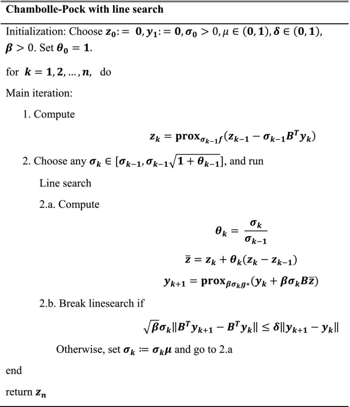
After knowing the proximal operator of the function f and g, the problem (B4) can be solved by a first order primal‐dual algorithm known as Chambolle–Pock algorithm.²⁹ A Chambolle–Pock algorithm with line search is used in this work, which follows the steps shown in Table BI.

Table BI.

Pseudo code for Chambolle–Pock with line search

References

- 1. Wilson RR. Radiological use of fast protons. Radiology. 1946;47:487–491. [DOI] [PubMed] [Google Scholar]
- 2. Liu W, Zhang X, Li Y, Mohan R. Robust optimization of intensity modulated proton therapy. Med Phys. 2012;39:1079–1091. [DOI] [PMC free article] [PubMed] [Google Scholar]
- 3. Albertini F, Bolsi A, Lomax AJ, Rutz HP, Timmerman B, Goitein G. Sensitivity of intensity modulated proton therapy plans to changes in patient weight. Radiother Oncol. 2008;86:187–194. [DOI] [PubMed] [Google Scholar]
- 4. Lomax AJ. Intensity modulated proton therapy and its sensitivity to treatment uncertainties 1: the potential effects of calculational uncertainties. Phys Med Biol. 2008;53:1027–1042. [DOI] [PubMed] [Google Scholar]
- 5. Lomax AJ. Intensity modulated proton therapy and its sensitivity to treatment uncertainties 2: the potential effects of inter‐fraction and inter‐field motions. Phys Med Biol. 2008;53:1043–1056. [DOI] [PubMed] [Google Scholar]
- 6. Lomax AJ, Boehringer T, Coray A, et al. Intensity modulated proton therapy: a clinical example. Med Phys. 2001;28:317–324. [DOI] [PubMed] [Google Scholar]
- 7. Unkelbach J, Chan TCY, Bortfeld T. Accounting for range uncertainties in the optimization of intensity modulated proton therapy. Phys Med Biol. 2007;52:2755–2773. [DOI] [PubMed] [Google Scholar]
- 8. Unkelbach J, Bortfeld T, Martin BC, Soukup M. Reducing the sensitivity of IMPT treatment plans to setup errors and range uncertainties via probabilistic treatment planning. Med Phys. 2009;36:149–163. [DOI] [PMC free article] [PubMed] [Google Scholar]
- 9. Albertini F, Hug EB, Lomax AJ. Is it necessary to plan with safety margins for actively scanned proton therapy? Phys Med Biol. 2011;56:4399–4413. [DOI] [PubMed] [Google Scholar]
- 10. Park PC, Zhu XR, Lee AK, et al. A beam‐specific planning target volume (PTV) design for proton therapy to account for setup and range uncertainties. Int J Radiat Oncol Biol Phys. 2012;82:e329–e336. [DOI] [PMC free article] [PubMed] [Google Scholar]
- 11. Bangert M, Hennig P, Oelfke U. Analytical probabilistic modeling for radiation therapy treatment planning. Phys Med Biol. 2013;58:5401–5419. [DOI] [PubMed] [Google Scholar]
- 12. Wahl N, Hennig P, Wieser HP, Bangert M. Efficiency of analytical and sampling‐based uncertainty propagation in intensity‐modulated proton therapy. Phys Med Biol. 2017;62:5790–5807. [DOI] [PubMed] [Google Scholar]
- 13. Gordon JJ, Sayah N, Weiss E, Siebers JV. Coverage optimized planning: probabilistic treatment planning based on dose coverage histogram criteria. Med Phys. 2010;37:550–563. [DOI] [PMC free article] [PubMed] [Google Scholar]
- 14. Pflugfelder D, Wilkens JJ, Szymanowski H, Oelfke U. Quantifying lateral tissue heterogeneities in hadron therapy. Med Phys. 2007;34:1506–1513. [DOI] [PubMed] [Google Scholar]
- 15. Bueno M, Paganetti H, Duch MA, Schuemann J. An algorithm to assess the need for clinical Monte Carlo dose calculation for small proton therapy fields based on quantification of tissue heterogeneity. Med Phys. 2013;40:081704. [DOI] [PubMed] [Google Scholar]
- 16. Toramatsu C, Inaniwa T. Beam angle selection incorporation of anatomical heterogeneities for pencil beam scanning charged‐particle therapy. Phys Med Biol. 2016;61:8664–8675. [DOI] [PubMed] [Google Scholar]
- 17. Liu W, Mohan R, Park P, et al. Dosimetric benefits of robust treatment planning for intensity modulated proton therapy for base‐of‐skull cancers. Pract Radiat Oncol. 2014;4:384–391. [DOI] [PMC free article] [PubMed] [Google Scholar]
- 18. Liu W, Frank SJ, Li X, Li Y, Zhu RX, Mohan R. PTV‐based IMPT optimization incorporating planning risk volumes vs robust optimization. Med Phys. 2013;40:021709. [DOI] [PMC free article] [PubMed] [Google Scholar]
- 19. Pflugfelder D, Wilkens JJ, Oelfke U. Worst case optimization: a method to account for uncertainties in the optimization of intensity modulated proton therapy. Phys Med Biol. 2008;53:1689–1700. [DOI] [PubMed] [Google Scholar]
- 20. Fredriksson A, Forsgren A, Hårdemark B. Minimax optimization for handling range and setup uncertainties in proton therapy. Med Phys. 2011;38:1672–1684. [DOI] [PubMed] [Google Scholar]
- 21. Fredriksson A, Bokrantz R. A critical evaluation of worst case optimization methods for robust intensity‐modulated proton therapy planning. Med Phys. 2014;41:081701. [DOI] [PubMed] [Google Scholar]
- 22. Chen W, Unkelbach J, Trofimov A, et al. Including robustness in multi‐criteria optimization for intensity‐modulated proton therapy. Phys Med Biol. 2012;57:591–608. [DOI] [PMC free article] [PubMed] [Google Scholar]
- 23. Stuschke M, Kaiser A, Pöttgen C, Lübcke W, Farr J. Potentials of robust intensity modulated scanning proton plans for locally advanced lung cancer in comparison to intensity modulated photon plans. Radiother Oncol. 2012;104:45–51. [DOI] [PubMed] [Google Scholar]
- 24. Casiraghi M, Albertini F, Lomax AJ. Advantages and limitations of the “worst case scenario” approach in IMPT treatment planning. Phys Med Biol. 2013;58:1323–1339. [DOI] [PubMed] [Google Scholar]
- 25. Li Y, Niemela P, Liao L, et al. Selective robust optimization: a new intensity‐modulated proton therapy optimization strategy. Med Phys. 2015;42:4840–4847. [DOI] [PubMed] [Google Scholar]
- 26. Unkelbach J, Alber M, Bangert M, et al. Robust radiotherapy planning. Phys Med Biol. 2018;63:22TR02. [DOI] [PubMed] [Google Scholar]
- 27. Xing L, Boyd S. Real‐time radiation treatment planning with optimality guarantees via cluster and bound methods problem description; 2017:1–24.
- 28. Beck A, Teboulle M. A fast iterative shrinkage‐thresholding algorithm for linear inverse problems. SIAM J Imaging Sci. 2009;2:183–202. [Google Scholar]
- 29. Chambolle A, Pock T. A first‐order primal‐dual algorithm for convex problems with applications to imaging. J Math Imaging Vis. 2011;40:120–145. [Google Scholar]
- 30. Cisternas E, Mairani A, Ziegenhein P, Jäkel O, Bangert M. matRad – a multi‐modality open source 3D treatment planning toolkit. In: IFMBE Proceedings (Vol. 51); 2015:1608–1611. 10.1007/978-3-319-19387-8_391 [DOI]
- 31. Wieser HP, Cisternas E, Wahl N, et al. Development of the open‐source dose calculation and optimization toolkit matRad. Med Phys. 2017;44:2556–2568. [DOI] [PubMed] [Google Scholar]
- 32. Grégoire V, Mackie TR. State of the art on dose prescription, reporting and recording in Intensity‐Modulated Radiation Therapy (ICRU report No. 83). Cancer/Radiother. 2011;15:555–559. [DOI] [PubMed] [Google Scholar]
- 33. Jia X, Schümann J, Paganetti H, Jiang SB. GPU‐based fast Monte Carlo dose calculation for proton therapy. Phys Med Biol. 2012;57:7783–7797. [DOI] [PMC free article] [PubMed] [Google Scholar]
- 34. Giantsoudi D, Schuemann J, Jia X, Dowdell S, Jiang S, Paganetti H. Validation of a GPU‐based Monte Carlo code (gPMC) for proton radiation therapy: clinical cases study. Phys Med Biol. 2015;60:2257–2269. [DOI] [PMC free article] [PubMed] [Google Scholar]
- 35. Qin N, Botas P, Giantsoudi D, et al. Recent developments and comprehensive evaluations of a GPU‐based Monte Carlo package for proton therapy. Phys Med Biol. 2016;61:7347–7362. [DOI] [PMC free article] [PubMed] [Google Scholar]
- 36. devan Water S , van Dam I, Schaart DR, Al‐Mamgani A, Heijmen BJM, Hoogeman MS. The price of robustness; impact of worst‐case optimization on organ‐at‐risk dose and complication probability in intensity‐modulated proton therapy for oropharyngeal cancer patients. Radiother Oncol. 2016;120:56–62. [DOI] [PubMed] [Google Scholar]
- 37. Shan J, Sio TT, Liu C, Schild SE, Bues M, Liu W. A novel and individualized robust optimization method using normalized dose interval volume constraints (NDIVC) for intensity‐modulated proton radiotherapy. Med Phys. 2018;00:00–00. [DOI] [PubMed] [Google Scholar]
- 38. Liu W, Li Y, Li X, Cao W, Zhang X. Influence of robust optimization in intensity‐modulated proton therapy with different dose delivery techniques. Med Phys. 2012;39:3089–3101. [DOI] [PMC free article] [PubMed] [Google Scholar]
- 39. Gu W, O'Connor D, Nguyen D, et al. Integrated beam orientation and scanning‐spot optimization in intensity‐modulated proton therapy for brain and unilateral head and neck tumors. Med Phys. 2018;45:1338–1350. [DOI] [PMC free article] [PubMed] [Google Scholar]
- 40. Boyd S, Vandenberghe L. Convex Optimization. Cambridge, MA: Cambridge University Press; 2010. 10.1080/10556781003625177 [DOI] [Google Scholar]