MR Fingerprinting with Simultaneous T₁, T₂, and Fat Signal Fraction Estimation with Integrated B₀ Correction Reduces Bias in Water T₁ and T₂ Estimates

Abstract

Purpose:

MR fingerprinting (MRF) sequences permit efficient T₁ and T₂ estimation in cranial and extracranial regions, but these areas may include substantial fat signals that bias T₁ and T₂ estimates. MRI fat signal fraction estimation is also a topic of active research in itself, but may be complicated by Bo heterogeneity and blurring during spiral k-space acquisitions, which are commonly used for MRF. An MRF method is proposed that separates fat and water signals, estimates water T₁ and T₂, and accounts for B₀ effects with spiral blurring correction, in a single sequence.

Theory and Methods:

A k-space-based fat-water separation method is further extended to unbalanced steady-state free precession MRF with swept echo time. Repeated application of this k-space fat-water separation to demodulated forms of the measured data allows a B₀ map and correction to be approximated. The method is compared with MRF without fat separation across a broad range of fat signal fractions (FSFs), water T₁s and T₂s, and under heterogeneous static fields in simulations, phantoms, and in vivo.

Results:

The proposed method’s FSF estimates had a concordance correlation coefficient of 0.990 with conventional measurements, and reduced biases in the T₁ and T₂ estimates due to fat signal relative to other MRF sequences by several hundred ms. The B₀ correction improved the FSF, T₁, and T₂ estimation compared to those estimates without correction.

Conclusion:

The proposed method improves MRF water T₁, and T₂ estimation in the presence of fat and provides accurate FSF estimation with inline B₀ correction.

1. INTRODUCTION

Water T₁, and T₂ and fat content are important for tissue characterization in MRI. For example, T₁, and T₂ values are altered in several diseased states, such as cardiac[1,2], liver[3], muscular[4], and others[5,6], in which the affected organs may contain or be near adipose tissue. The MRI-estimated fat signal fraction (FSF) is important in studies of healthy and pathological function, including brown adipose tissue[7] and abdominal organs[8–10]. One approach to time-efficient, multi-parametric quantitative MRI is unbalanced steady-state (uSSFP) MR fingerprinting (MRF). uSSFP-MRF permits the rapid, simultaneous estimation of T₁, and T₂ by acquiring signals over a train of pseudo-random nutation angles and TR values.[11] This sequence has been applied to study regions with potential ectopic and visceral fat such as the abdomen[12], prostate[13] and heart[14].

In both conventional MRI and MRF, fat signals confound T₁, and T₂ estimates. The methylene peak of fat often has a shorter T₁ and longer T₂ than water[15,16]. Partial volume effects of fat may bias MRI T₁ estimates in the breast[17] and liver[18] and T₂ estimates in muscle[4]. Conventional MRI relaxometry approaches that exclude fat often rely on separate inversion recovery preparation, composite pulses, or chemically selective pulses to suppress the fat signal. Such techniques may increase the scan duration through their preparation or timing requirements, partially saturate water signal, inaccurately assume a single peak model for fat, or have sensitivity to non-ideal B₀ or B₁+[19]. Conversely, conventional Dixon MRI fat-water estimation is not generally employed to estimate longitudinal and spin-spin relaxation. Also, heterogeneous B₀ makes fat-water separation a non-linear optimization problem[20]. This has been solved by a number of different approaches[20–23], but these techniques generally assume a steady-state water signal, apart from B₀ effects. MRF uses non-steady-state water/fat signals to estimate T₁ and T₂ from the signal dynamics over many TRs. Because typical fat-water separation does not account for variable flip angles, the use of non-steady state signals may confound fat-water separation if a single, variable TE is acquired at each TR.

While the biases in T₁ and T₂ estimation due to fat have not been explicitly considered using MRF, MRF-based fat-water separation has been explored. The original MRF approach, based on balanced SSFP, permitted fat signal estimation through its sensitivity to off-resonance/relaxation effects[24]. However, partial volume effects were not considered. Cloos et al. explored fat imaging in the thighs using a two-point Dixon approach with a radial acquisition[25]. Several preliminary works have explored fat-water separation in uSSFP-MRF[26–30]. Very recently, simultaneous fat-separated T₁, B₁+, and B₀ estimation has been demonstrated at 1.5 T using MRF[31]. Yet, we are unaware of a full paper that has described an MRF approach for separating fat and water signals while simultaneously estimating the water-only T₁ and T₂ with B₀ correction.

Spiral acquisitions are commonly used in MRF, further complicating parameter estimation by introducing blurring from chemical shift and B₀ effects[27]. While spiral blurring with fat-water separation remains an active topic of research[32], fat blurring in MRF spiral acquisition is relatively unexplored. Spiral blurring effects can be limited by using lower field strength, reduced spiral acquisition time, or radial acquisitions. However, these techniques lower the signal-to-noise ratio or restrict the timing of the image encoding.

The first goal of this work is to illustrate the potential for bias in MRF-derived T₁ and T₂ estimates of tissues containing composite fat-water signals. We introduce an MRF method that separates fat and water signals, allowing B₀-corrected water T₁ and T₂ estimates with reduced levels of bias, as well an estimate of FSF. To do so, we propose modifications to the original uSSFP-sequence and reconstruction. By using a swept echo time and integrating a previously reported B0 correction method[33,34] into the reconstruction pipeline, we reformulate the parameter estimation problem into an optimization for B₀. This optimization, along with an assumed multi-spectral fat model, results in corrected water and fat signal estimates. The outputs of the proposed approach are B₀-corrected, fat-separated water T₁ and T₂ maps and an FSF map with spiral deblurring.

2. THEORY

We will first show that we can extend a k-space-based fat-water separation technique to MRF. We will then show that we can simultaneously estimate B₀ with fat-water separation with variable TE- and fixed TR-MRF sequences using a form of conjugate phase reconstruction.

2.1. MRF k-Space Fat-Water Separation

Brodsky et al.[35] showed that k-space-based fat-water separation is possible using a linear system of equations. We can extend this technique to MRF. An MRF signal vector through all N TRs not subject to B₀ deviations, s_o(k) ∈ ℂ^N, at a given k-space position k can be closely approximated as

$${\mathbf{s}}_o(\mathbf{k})\approx A_k\mathbf{b}(\mathbf{k})$$ [1]

where A_k is the k-space position dependent system matrix and b(k) ∈ ℂ^M+1 are the coefficients that describe the water and fat components, with M defined below. A subscript on s is used to specify that B₀ effects outside of chemical shift are not considered in this model.

The system matrix in Eq. (1) can be given as

$$A_k=\left[{\mathbf{u}}_1\cdots {\mathbf{u}}_M|\mathbf{g}(t(\mathbf{k}))\right]$$ [2]

where $A_k\in {ℂ}^{Nx(M+1)}$, $\left\{{\mathbf{u}}_m\right\}\in {ℂ}^{Nx1}$ are k-space independent singular vectors which describe the water dictionary in the time domain, and g(t(k)) is the fat model with k-space dependence through the finite trajectory timing (further defined below). McGivney et al. [36] showed that the water dictionary is highly compressible in the time dimension. Since the compressibility of the water dictionary, as measured by the singular values, is invariant under transpose, we can similarly reason that the parameter dimension of the water dictionary is compressible. The vectors {u_m} can be calculated by singular value decomposition (SVD) of the water dictionary, using the left singular vectors to form {u_m} (for a dictionary ∈ ℂ^NxQ with Q dictionary atoms). The value of M, the number of members in the set {u_m}, is determined by the fraction of singular value energy one wishes to retain. Increasing the value of M, increases the model accuracy of Eqs. (1) and (2). The last column of A_k describes the MRF fat model in k-space, g(t(k)) ∈ ℂ^Nx1, with the n^th element of g given as

$${\text{g}}_n(t(\mathbf{k}))=\frac{1}{b_o(\mathbf{k})}\sum _{p=1}^{p=P}{b}_{p,n}{e}^{i2\pi f_p\left(T{E}_n+t(\mathbf{k})\right)}$$ [3].

Here b_o(k) is a k-space dependent normalization factor that gives g(t(k)) unit norm, b_p,n a triglyceride peak weighting that accounts for MRF sequence T₁/T₂ contrast effects for TR_n and the moiety’s weighting relative to the whole triglyceride, f_p is the p^th peak’s chemical shift frequency, TE_n is the echo time for TR_n, and t(k) is the time to reach k through the k-space trajectory. In this work, we assume that the echo time starts at the beginning of the spiral readout at the k-space origin. The coefficient estimates at each k-space position, $\hat{\mathbf{b}}$(k) ∈ ℂ^M+1, may be solved by pseudo-inverse of A_k using Eq. (1).

The water dictionary does not contain phase evolution through time, and {u_m} are orthonormal by definition. The fat signal, g, does exhibit complex periodic phase through time that lends a certain amount of orthogonality to the water dictionary basis. As a result, we find that the conditioning of is A_k is reasonable throughout k-space for the trajectory timing and TEs used in this work.

The Fourier transform of $\hat{\mathbf{b}}$(k) gives coefficient images represented by $\hat{\mathbf{b}}$(r), for a given spatial position r. These images are representations of the coefficients in the spatial domain. The coefficients in the spatial domain can then be multiplied by the water ({u_m}) and fat (g) model vectors at each r to reconstruct the estimated MRF water and fat signals. The fat coefficient estimate, the last entry of $\hat{\mathbf{b}}$(r), is multiplied by g with t = 0 in Eq. (3). Under this condition, A_k = A is independent of k-space and can be applied in the image domain to on-resonance signals. This reconstructed representation of the MRF fat signal does not exhibit blurring due to chemical shift, since the phase accrual in k-space has been fit using Eq. (3). While this fat-water separation does resolve blurring due to chemical shift, it does not consider B₀ effects that may confound the fat-water fitting due to blurring or frequency shift.

2.2. B₀ Fitting with MRF Fat-Water Separation

We can extend the concept of a conjugate phase reconstruction technique called multi-frequency interpolation (MFI)[33,34] to correct for B₀ blurring and fat-water separation bias. If the MRF TRs are fixed, the uSSFP MRF sequence will refocus off-resonance magnetization contributing to signal at the beginning of every TR[37,38]. If the TE is varied linearly, using MFI, the demodulated MRF signal in the image domain s_o(r) at position r is

$${\mathbf{s}}_o(\mathbf{r})\approx \sum _{l=1}^{l=L}{a}_l\left(\mathbf{r};B_o(\mathbf{r})\right)s_l(\mathbf{r})$$ [4]

where {a_l(r)} depend only on B_o(r) and (s_l(r)} are image domain MRF signals from the Fourier transforms (ℱ) of the corresponding k-space representations of the demodulated MRF signals {s_l(k)}. That is,

$${\text{s}}_{n,l}(\mathbf{r})={\mathfrak{F}}^{-1}\left\{{\text{s}}_{n,l}(\mathbf{k})\right\}={\mathfrak{F}}^{-1}\left\{e^{-i2\pi f_l\left(T{E}_n+t(\mathbf{k})\right)}{s}_n(\mathbf{k})\right\}$$ [5]

where f_l is the l^th MFI basis frequency. The accuracy of Eq. (4) is limited by the number of basis frequencies used, as well as[39,40] by non-zero B₀ gradients. Eq. (4) can be used to help determine an estimate of B_o(r) in the presence of fat as follows.

If we enforce consistency between the spatial representation of Eq. (1) and Eq. (4), and apply variable projection, we can form an objective function that depends on B_o(r) and the given measurement. The problem statement is

$${\widehat{B}}_0(\mathbf{r})=\underset{B_0}{\arg \min }{\Vert \left[I-A{A}^{†}\right]\sum _{l=1}^L{a}_l\left(B_0(\mathbf{r})\right){\mathbf{s}}_l(\mathbf{r})\Vert }_2^2$$ [6].

A^† denotes the pseudo-inverse of A (Eq. (2)). Here, we have used the standard signal model assumption that the image is instantaneously acquired at the echo time. As mentioned above, the matrix A can be applied in the image domain by letting t = 0 in Eq. (3). The definition and dimensions of A are otherwise the same as in Eq. (2).

The memory requirements implied by Eq. (6) may be reduced by SVD compression. Depending on the number of MFI basis frequencies, L, solution implementation requires enough memory to store L MRF data sets. To reduce this, a basis set of orthonormal vectors, stored in a matrix U ∈ ℂ^NxM’ that describe any relevant s_l, can be formed by SVD of an MRF dictionary that includes off-resonance/chemical shift effects. The number of columns M’ in U is defined similarly to M, as the number of singular values necessary to capture a specified singular value energy. A set of coefficients {c_l(k)} that describe s_l(k) is given as

$${\mathbf{c}}_l(\mathbf{k})=U^H{\mathbf{s}}_l(\mathbf{k})$$ [7].

The spatial representations of these coefficients c_l(r) can be calculated as the Fourier transform of their k-space representations. Combining Eq. (6) and (7) gives

$${\widehat{B}}_0(\mathbf{r})=\underset{B_0}{\arg \min }{\Vert \left[I-A{A}^{†}\right]\sum _{l=1}^L{a}_l\left(B_0(\mathbf{r})\right)U{\mathbf{c}}_l(\mathbf{r})\Vert }_2^2$$ [8].

Eq. (8) can be solved by exhaustive search as discussed in Methods. MRF is known to estimate T₁ and T₂ accurately despite undersampling factors as large as 48.[11] Similarly, we test if the above expressions yield accurate fat-water separation with B₀ compensation in highly aliased/undersampled MRF data using the following phantom and in vivo experiments.

3. MATERIALS AND METHODS

3.1. MRF Image Acquisition and Processing

3.1.1. MRF sequences

To implement the proposed solution and compare it to standard MRF approaches, we designed three different MRF sequences. The proposed sequence permits chemical shift encoding through variable TE. The next two sequences, based on standard MRF approaches, have fixed TE and do not encode chemical shift information. All sequences used adiabatic inversion with an inversion time (TI) of 40 ms, excitation with a sinc-gauss pulse and a time-bandwidth product of 1o to minimize B₁+ heterogeneity in the slice profile[41] and slice thicknesses of 5 to 30 mm (see below). Images were encoded using a numerically optimized spiral[42] with a fixed undersampling factor of 32, an acquisition time of approximately 5 ms and rotated 11.25° between TRs. In-plane image resolution ranged from 1.0 to 1.5 mm (see below).

The three MRF sequences differed as follows. The proposed variable TE uSSFP MRF sequence (MRF-varTE) used 1500 TRs, fixed TR of 16 ms, a linearly swept TE from 3.5 to 7.5 ms over the 1500 TRs, fixed radiofrequency phase and a variable flip angle pattern (Supplementary Fig. S1). The flip angle pattern was designed from half-sinusoids with randomly varying maximum amplitudes[11] no greater than 60°. The scan duration was 24 s. The first fixed TE uSSFP MRF sequence (MRF-fixTE) used 1500 TRs, fixed TR of 16 ms, a TE of 4.65 ms, and the same flip angle pattern as MRF-varTE, for a scan duration of 24 s. The second fixed TE MRF sequence used a variable TR (MRF-varTR) with variable flip angle and TR patterns (Supplementary Fig. S2) with fixed TE = 3.5 ms, adapted from the first MRF uSSFP (FISP) sequence[11]. The scan duration was 17.5 s.

All images were acquired on a 3T Philips Ingenia (Philips Healthcare, The Netherlands) with a 32-channel head coil for phantom experiments and brain acquisitions, a 16-channel transmit-receive knee coil for knee acquisitions, and a multi-channel anterior coil with integrated tabletop posterior coil for abdominal acquisitions.

3.1.2. Image reconstruction and MRF T₁/T₂ estimation

Following k-space data acquisition, we reconstructed the undersampled MRF data using iterative sample density compensation[43] derived from fully-sampled k-space coordinates combined with SVD virtual coil compression by a factor of two, sensitivity map estimation using eSPIRIT[44], and gridding and coil combination using the Berkeley Advanced Reconstruction Toolbox (BART)[45]. The k-space trajectory was measured using an implementation[46] of the Duyn method[47]. The input for eSPIRIT used low resolution reconstructions generated from the inner 30×30 grid of k-space positions of each virtual coil’s MRF image stack. All processing was performed in MATLAB (The MathWorks, Natick, MA, USA).

Estimates for T₁/T₂ were made in the following way. We used an extended phase graph algorithm[48] to construct an on-resonance water dictionary using the following range of T₁, T₂, and B₁+ values: (min:step:max): T₁ (ms) 10:10:90, 100:20:1000, 1040:40:2000, 2050:100:3000; T₂ (ms) 2:2:8, 10:5:100, 110:10:300, 350:50:800, 900:100:1500 (adapted from Ref[49]); B₁+ 0.5, 0.6, 0.7 0.75, 0.8:0.025:1.2, 1.25 1.3, 1.4, 1.5. MRF-fixTE and MRF-varTR T₁s and T₂s were fitted using the inner product of the compressed signal and time-compressed dictionary[36] constrained from independently measured 3D B₁+ map using the Yarnykh[50] method (except as noted) with high in-plane (2×2 mm²) resolution and a 1.5–2 min acquisition time to ensure sufficient SNR. MRF-varTE water T₁s and T₂s were estimated in the same way, but using the water signal following fat-water separation.

3.1.3. Implementation of MRF Fat-Water Separation

Figure 1 provides a flowchart describing the fundamental steps of the proposed solution. The basic workflow is to reconstruct and combine coil images, perform a demodulation in k-space using the MFI basis frequencies, do a k-space fat-water separation, and then transform to the image domain and fit a B₀ map that yields the B₀-corrected coefficients used to reconstruct the fat and water signals.

Fig. 1.

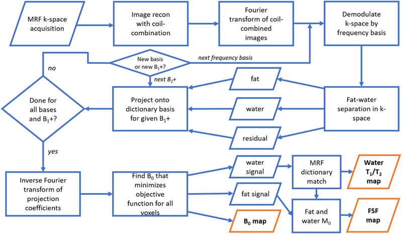
A flowchart of the implementation for the proposed MR fingerprinting (MRF) fat-water separation technique. A fixed-TR, linear swept TE is used for the MRF acquisition. Following gridding and coil-combination, the MRF stack is transformed back into k-space and demodulated as described in the Theory section. Fat-water-residual separation is performed in k-space for each demodulation frequency and each discretized B₁+. The water, residual, and deblurred fat components are projected onto an approximate basis of a dictionary that includes T₁, T₂, and off-resonance effects. The coefficients of this projection are transformed to the image domain and smoothed (not shown), and B₀ at each voxel is fitted. The B₀ estimate is then used to appropriately combine the water and fat coefficients to yield fat signal fraction (FSF), and water T₁ and T₂ maps.

The gridded and coil-combined k-space data were demodulated for each basis frequency and then separated into their fat-water-residual components. We defined basis frequencies as the 31 central Fourier basis frequencies over the time interval from TE = 0 to 20% larger than the sum of the latest TE and spiral acquisition time, discretized into the number of spiral read points from a single interleaf with apodization as originally described for MFI[33]. This produced coefficients for B₀ values with normalized RMSE <1.5% over a frequency range of ±700 Hz within the shortest TE to the longest TE plus the spiral acquisition time. This bandwidth is sufficient to capture chemical shift combined with significant B₀ effects. The number of basis vectors in U (in Eqs. 7 and 8) and in {u_m} (in Eq. (2)) were defined as the rank of the SVD of the respective dictionaries that captured 99.99% of the singular value energy. The multi-peak fat model was defined as in Eq. (3) and used previously reported chemical shifts and estimated T₁/T₂ values of white adipose tissue[15] (Supplementary Table S1). The fat-water fit was repeated for all discretized B₁+ values. The resulting fits and residuals were projected on the off-resonance dictionary basis for each voxel in gridded k-space for each discretized B₁+ value and frequency demodulation. The k-spaces of the fit coefficients were then converted to the image domain.

Following fat-water separation for all of k-space and conversion to the image domain, we smoothed the coefficient maps using a Gaussian kernel of 1.5 voxels. It was found empirically that this smoothing removed single voxel outliers in the B₀ fits. We then fit for the B₀ map.

The B₀ fitting was performed using Eq (8). The possible B₀ values were discretized by 10 Hz increments and restricted to a range of ±250 Hz. For each voxel, linear combinations of the reconstructed signal were made with the precalculated coefficients (a_l(B_o)} for all discretized B₀ values to determine the B₀ that minimized the objective function as stated in Eq. (8). The B₀-corrected water signal T₁ and T₂ values were estimated as described above. The water (W) and fat (F) magnitudes for each voxel were defined as their respective M₀ estimates. M₀ for fat and water were calculated as the complex inner product of the B₀-corrected fat and water signal estimates with their respective signal models. The FSF at each voxel was given as

$$FSF=\frac{F}{W+F}$$ [9].

3.1.4. Dictionary MRF fat-water separation

To compare with the proposed solution, we implemented an MRF fat-water separation in the image domain using an MRF dictionary with fat signal, without adjusting for spiral blurring. The fat-water dictionary was composed of discretized FSF (0.0:0.05:1.0) using linear combinations[27] of the water dictionary and the multi-peak fat model with the MRF-varTE sequence. Reconstructed MRF images were then matched to the fat-water dictionary on a voxelwise basis to estimate water T₁, water T₂, and FSF.

3.2. Simulation Studies

3.2.1. Simulation of T₁ and T₂Bias Due to Fat

To understand better the potential for fat bias in MRF T₁ and T₂ estimates under ideal conditions, we numerically simulated fully-sampled MRF-varTE, MRF-fixTE and MRF-varTR signals. We then estimated the T₁ and T₂ for all sequences with fat-water separation for MRF-varTE and without fat-water separation for MRF-fixTE and MRF-varTR. The multi-peak fat model was defined as above. Linear combinations of the normalized fat and water signals with varying FSFs were simulated and matched against the water dictionary. The following T₁/T₂ combinations and FSF values were simulated: 500/30, 800/30, 1200/50, 1600/100, 2250/100 ms and FSF 0.0:0.05:1.0. The simulation assumed zero noise. T₁ and T₂ were estimated as described above.

3.2.2. MRF Image Simulations

To assess the performance of the proposed method relative to MRF T₁ and T₂ estimation methods that do not account for fat, simulated measurements with undersampling and varying levels of noise were generated from a digital phantom. Since we were unaware of any consensus digital fat phantoms with varying water T₁ and T₂, we used a digital 240 × 240 Shepp-Logan phantom and arbitrarily assigned different segments of the phantom an FSF and one of the T₁/T₂ combinations used in §3.2.1. The FSF values were 0.0, 0.25, 0.5, 0.6, and 0.8. The total magnetization density was kept uniform throughout the image. The parameter assignments to each phantom segment are detailed in Supplementary Fig. S3 and Supplementary Table S2. All simulated MRF stacks were subjected to 150 Hz off-resonance.

The undersampled spiral MRF acquisitions were simulated as described by Zhao et al[51]. Undersampled spiral images were generated by non-uniform fast Fourier transform[52] from a measured k-space trajectory used in this study. Blurring effects from chemical shifts and off-resonance were simulated using a spiral acquisition time of 5.0 ms and the measured trajectory. Complex white Gaussian noise values were added in k-space to yield SNR values of 28, 32, and 38 dB as well as no added noise, as described in Ref[51]. All parameters were estimated for the proposed fat-water separation method using the MRF-varTE simulations. T₁ and T₂ were estimated without fat separation for the MRF-fixTE and MRF-varTR simulations. Parameter bias for each voxel was calculated as the difference from ground truth. Uncertainty was quantified as the standard deviation (SD) of voxel bias to permit comparison of segments with differing T₁/T₂. Mean bias and SD of the bias were calculated for the entire non-zero image defined by ground truth.

3.3. Phantom Experiments

3.3.1. FSF Estimation with MRF Direct Match vs. k-Space Fitting

The proposed method, as well as a dictionary-based fat estimation, were used to measure FSF in a fat-water phantom. The phantom was composed of 50 mL conical centrifuge tubes filled with differing concentrations of peanut oil and aqueous agar doped with a gadolinium-based contrast agent.

The phantom was imaged with the MRF-varTE and spoiled gradient echo (SGPR) sequences. The images were reconstructed as described above, with an FOV of 240 × 240 mm², in-plane resolution of 1 × 1 mm² and slice thickness of 8 mm. A 3D spoiled gradient echo (SPGR) sequence with 6 TEs (TE_min = 1.5 ms, ΔTE = 1.1 ms) with a flip angle of 3° was acquired and processed with a graph cut-based fat-water separation algorithm with simultaneous B₀ and R₂* correction[22], serving as FSF reference. The FSF was also estimated from MRF-varTE using the proposed solution and the dictionary-based fat-water separation.

The concordances of the two MRF FSF estimation methods with the SPGR reference were calculated. ROIs were manually drawn within each imaged phantom tube on a SPGR reference image. The means of the ROIs’ FSFs were used to calculate the concordance correlation coefficients (CCC)[53] for the two MRF methods.

3.3.2. Variability of Water T₁ and T₂ Estimation with Partial Volume of Oil

We constructed a phantom of distinct water and oil compartments with varying water T₁ and T₂ to test the proposed method across a broad range of water contrasts. Nine 50 mL conical centrifuge tubes were filled with 25 mL of deionized water with different concentrations of MnCl₂, over which 25 mL of peanut oil were added. This produced separated water and oil layers in each tube (Supplementary Fig. S4). The tubes were then placed in a rectangular plastic container filled with a 2% aqueous agar gel to serve as a background signal. This fat-water layer phantom was imaged in cross-section with 3 cm slice thickness. Seven slice offsets were used, generating a different FSF for each slice. This permitted different T₁ and T₂ combinations across seven different fat fractions.

At each offset, images were acquired with all MRF sequences and a 2D SPGR sequence with the same echo time spacing and in-plane resolution described in §3.3.1. The through-slice position of the SPGR sequence was corrected by 1.2 mm to adjust for the different positions of the bulk methylene-water interface relative to the different RF bandwidths of the MRF and reference SPGR sequences. This partially corrected for differences in the height of the oil-water interface from the different bandwidth pulses.

To assess the relative biases in water T₁ and T₂ estimation due to fat signal contamination, the deviations in each sequence’s T₁ and T₂ estimates from consensus values were calculated as functions of oil content. The T₁ and T₂ values were estimated by all three MRF sequences in a slice that contained only water. These were averaged to yield water T₁ and T₂ consensus values for each tube. For each slice and MRF sequence, the T₁ and T₂ consensus estimates from each tube were subtracted from estimates with different fat fractions to determine the relative bias in estimated T₁ and T₂ for each FSF and MRF sequence. The SPGR data with graph cut processing (as in §3.3.1) was calculated for all slices/fat fractions and tubes for reference FSF values.

The accuracies of T₁/T₂ estimates in water for all MRF sequences were separately verified in a NIST-traceable MRI system phantom (Supplementary Fig. S5).

3.3.3. Effect of B₀ on Proposed Method

To explore the effect of the in-line B₀ fitting, the oil-water layer phantom was imaged under heterogeneous B₀ conditions and processed with and without the proposed B₀ correction. Cross-sectional acquisitions with the MRF-varTE and 2D SPGR sequence were selected at a single slice to produce FSF values ranging from ~10–30% across the different phantom tubes. Pencil-beam shimming was used to produce a reference scan with minimal B₀ variation, then the shimming was manipulated to produce a heterogeneous off-resonance pattern. The MRF data were processed with k-space fat separation with and without the B0 fitting portion of the code, and the SPGR images were processed as in §3.3.1.

3.4. In Vivo Experiments

To assess the in vivo differences of the MRF methods, as well as the feasibility of the fat-water separation method proposed here, three subjects were imaged in three anatomical sites after providing informed consent and with the approval of the local institutional review board.

One subject was imaged in a sagittal plane in the left knee with all MRF sequences using in-plane resolution of 1 × 1 mm², 5 mm slice thickness, and an FOV 240 × 240 mm². For reference, we acquired the following scans: a six-echo 3D SPGR sequence with minimum TE = 1.4 ms and ΔTE = 1.1 ms; a fat-suppressed single-shot gradient echo inversion recovery (IR-TFE) sequence using a water excitation 1–3-3–1 binomial pulse, inversion times of 50, 100, 200, 500, 1000, 2000, and 6000 ms, and delay time (TD) of 2500 ms with 2 excitations; a fat-suppressed 20-echo multiple spin-echo (MSE) sequence using spectral adiabatic inversion recovery and extra olefinic saturation prepulse, Version S refocusing[54], minimum TE = 20 ms, echo spacing 20 ms, TR = 3000 ms; and T₁-weighted turbo spin echo (TSE) sequence with a TR/TE = 700/11 ms and TSE factor of 3. Besides the in-plane resolution for the MSE and IR-TFE acquisitions of 2 × 2 mm², all other spatial resolutions and slice thickness equaled those of the MRF sequences. All reference scans were reconstructed to the same FOV and in-plane resolution as the MRF images. FSF estimates from the SPGR were made as described in §3.3.1. The proposed fat-water separation was performed for the MRF-varTE sequence. T₁ and T₂ estimates were made using the acquired images (MRF-fixTE, -varTR) and the water images (MRF-varTE) as described above. For the IR-TFE acquisition, T₁ was estimated using a non-linear fit to the magnitude images with the following three-parameter signal model[55]

$$S(TI)=\left|S_o\left[S_f\left(1-e^{\frac{-TD}{T_1}}\right)e^{\frac{-TI}{T_1}}+1-e^{\frac{-TI}{T_1}}\right]\right|$$ [10].

Here, S(TI)is the signal at TI, S_o is the equilibrium signal intensity, and S_f scales for imperfect inversion. T₂ was estimated from the magnitude MSE images using the following three parameter signal model

$$S(TE)=S_o{e}^{\frac{-TE}{T_2}}+{ϵ}_o$$ [11].

Here, S(TE) is the signal at the given TE, S_o is a scaling factor, and ∊_o accounts for a noise floor. To better evaluate parameter estimates, T₁ and T₂ maps were masked using the SPGR water image with a threshold based on Otsu’s method [56].

The second subject was also imaged with SPGR and MRF sequences in the transverse direction in the brain at the level of the orbits. The resolution, FOV and SPGR TEs were the same as those for the knee.

To provide proof-of-concept of the proposed method in a region sensitive to respiratory motion, the third subject was imaged in a transverse plane in the abdomen with the MRF-varTE sequence and processed with the proposed method. The resolution and FOV were 1.5 × 1.5 mm² with slice thickness 8 mm, and 480 × 480 mm², respectively. To permit faster acquisition, a B₁+ map was estimated using dual refocused echo acquisition mode sequence[57] with a scan duration of 8 s. Separate end-exhalation breath-holds were used for the MRF and B₁+ acquisitions.

4. RESULTS

4.1. Simulation Studies

Figure 2 shows the results of simulations of T₁ and T₂ biases due to fat for the different MRF sequences. The fitted Tis are unbiased for the MRF-varTE (with fat separation) for FSF < 1.0 (Fig. 2a). They decline approximately linearly for the MRF-fixTE sequence (Fig. 2b), and sharply increase then decrease for the MRF-varTR simulations (Fig. 2c). Biases without fat-separation exceed several hundred ms and even saturate for the MRF-varTR results at the 3000 ms limit of T₁ in the dictionary. The simulated water T₂ estimates are unbiased for the MRF-varTE with the proposed method (Fig. 2d) and vary for the MRF sequences without fat separation (Figs. 2e, f).

Fig. 2.

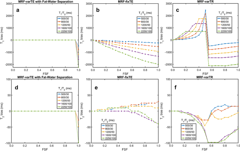
Simulated water T₁ and T₂ bias from fat using MRF sequences. This simulation used the variable TE MR fingerprinting (MRF) sequence with the proposed fat-water separation (MRF-varTE), as well as the fixed TE (MRF-fixTE) and fixed TE/variable TR MRF sequence (MRF-varTR) without fat-water separation. The simulated signals were fully sampled without blurring effects, noiseless and matched against a water-only dictionary for fat signal fractions (FSF) from 0.0 to 1.0 in increments of 0.05. The T₁ bias (a-c) and T₂ bias (d-f) for five listed T₁/T₂ combinations as a function of fat signal fraction (FSF) are shown. MRF-fixTE is in-phase with the main methylene peak of fat whereas MRF-varTR is approximately opposed phase. Water T₁ and T₂ bias in the proposed method (a, d) occur only when water is entirely absent (FSF = 1.0) and is otherwise zero. The T₁ positive bias is so large for the MRF varTR sequence (c) that it is saturated due to the maximum T₁ used in this study (3000 ms).

The image simulation results show that the proposed method reduces T₁ and T₂ bias and uncertainty, relative to MRF without fat separation. Figure 3 presents the ground truth and estimated parameters from all MRF sequences for the lowest SNR simulated (28 dB). Bias and blurring from fat signal and from off-resonance B₀ can be seen in the MRF-fixTE and MRF-varTR T₁ and T₂ maps. In comparison, the MRF-varTE parameter maps show closer agreement to the ground truth T₁ and T₂ as well as sharper geometric definition. The mean T₁ bias without fat separation drops from about −150 ms to less than 5 ms with fat separation (Fig. 3c). Bias reduction using the proposed method can also be observed for T₂. The standard deviations (SDs) of the bias for the proposed method are reduced by a factor of approximately three to five for T₂ and T₁, respectively (Fig. 3c). Decreases in SDs can be seen for the proposed method as the noise level decreases. The proposed technique has mean FSF estimation bias ≤ 0.017 (≤ 0.025 SD) and B₀ bias ≤ 1 Hz (≤ 6 Hz SD) for all noise levels. If the parameter estimates are made from fully-sampled and zero-noise images, the mean T₁ and T₂ biases and SDs drop to zero for the proposed method (Supplementary Figs. S6-S7). In contrast, the biases and SDs for the MRF estimates without fat separation approximately equal those from the undersampled, noisy simulations.

Fig. 3.

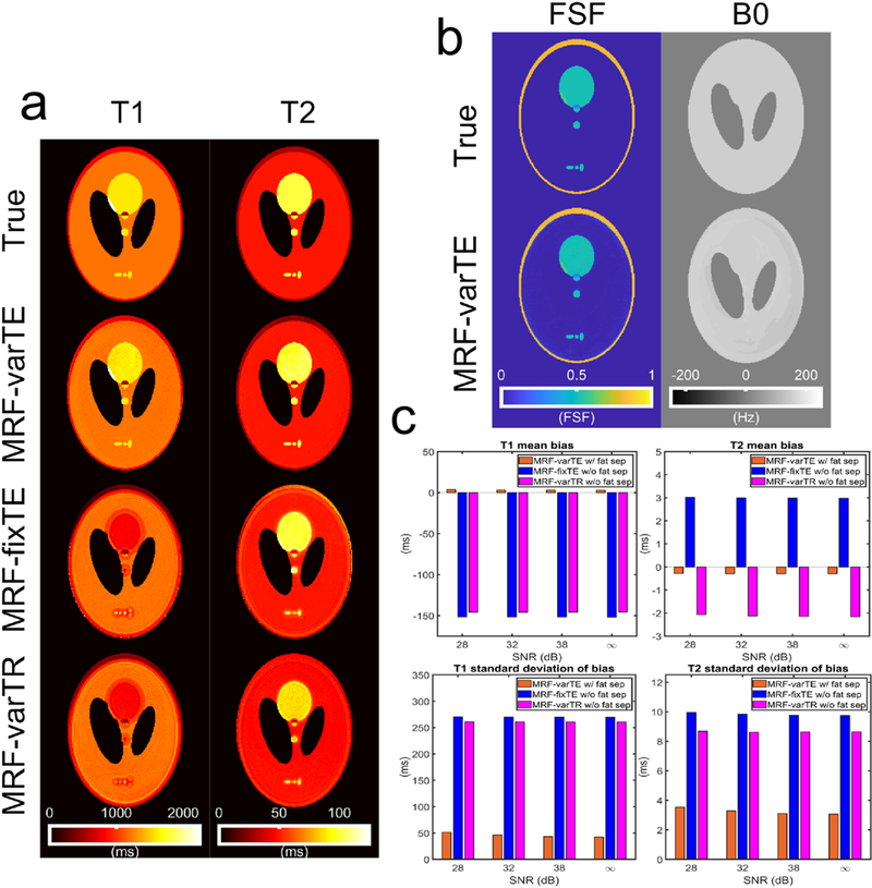
Example parameter estimates for the MR fingerprinting image simulations and associated bias plots. The example maps here use an SNR of 28 dB, an undersampling factor of 32, and a spiral acquisition time of 5.0 ms. The T₁ and T₂ maps (a) from the MRF-varTE sequence with fat separation exhibit reduced bias compared to the MRF-fixTE and MRF-varTR which do not use fat separation or account for spiral blurring due to B₀/fat chemical shift. The fat signal fraction and B₀ map for the MRF-varTE method (b) generally agrees with the ground truth. T1 and T2 estimation bias and the standard deviation of the bias are reduced at all noise levels for the MRF-varTE with fat separation simulations relative to the MRF techniques without fat separation (c).

4.2. Phantom Studies

The concordance of the dictionary and k-space MRF fat-separation methods with the SPGR-derived estimate for FSF exceeded 0.980 in both cases (Supplementary Fig. S8). However, the dictionary-based method has blurring artifacts on the outer edges of the phantom tubes due to the fat chemical shift. There are also asymmetric features that are likely due to B₀ inhomogeneity. The k-space method with B₀ correction FSF map does not show these artifacts.

The CCCs of all MRF and conventional T₁ and T₂ estimates in the MRI system phantom relative to specifications were ≥ 0.988 and ≥ 0.978, respectively (Supplementary Fig. S5).

For the oil-water phantoms, the T₁ and T₂ deviations from water reference values with increasing oil-fraction are smaller for the MRF-varTE than for the MRF methods without fat separation. Figure 4 shows example T₁ and T₂ maps in the water-only slice and a slice that contains ~30 to 50% fat signal. The water T₁s and T₂s range from approximately 300 to 1500 ms and 30 to 180 ms, respectively. The MRF T₁ and T₂ estimates in the water layer were consistent; the maximum absolute difference between each MRF sequence’s estimate and the averaged values for each tube were 17 ms and 3 ms for T₁ and T₂, respectively. The T₁ values for the oil-water slice are mostly lower than those from the water-only slice, with the MRF-varTR sequence changes being the most variable. The MRF-fixTE (Fig. 4e) and MRF-varTR (Fig. 4f) exhibit greater deviations than the MRF-varTE with fat separation (Fig. 4d). The T₂ maps in Fig. 4(g-l) appear to show slightly reduced, relatively unchanged, and widely varying changes in the oil-water slice relative to the water-only slice for the MRF-varTE with fat separation, MRF-fixTE and MRF-varTR, respectively. Figure 5 plots the differences in T₁ and T₂ estimates from the water-only slice consensus values for all tubes and all oil-water slices as a function of FSF (including water only). At FSF >0.15, much wider perturbations in estimated T₁ are seen with the MRF-fixTE and MRF- varTR than with MRF-varTE with fat separation. The T₂ deviations of the MRF-varTR are greater than those of the MRF-varTE and MRF-fixTE, whereas MRF-varTE deviations are more negative than those of MRF-fixTE. The general variation in T₁ with increasing FSF are similar to the simulation (Fig. 2) results for each sequence.

Fig. 4.

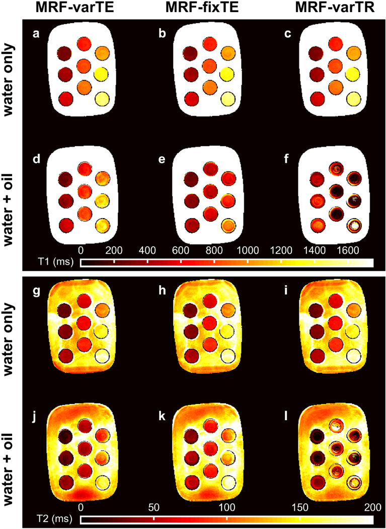
The MR fingerprinting (MRF) T₁ and T₂ maps from the oil-water phantom. The MRF-varTE sequence uses the proposed k-space fat-water separation whereas the MRF-fixTE and MRF-varTR sequences do not separate fat from water. The T₁ estimates from a pure water layer within the phantom tubes (a-c) are shown above the T₁ estimates from an oil-water layer (d-f). The T₂ estimates are arranged as the T₁ maps with water-only T₂ estimates in (g-i) above the oil-water T₂ estimates (j-l) and the same MRF sequence order from left to right. The largest deviations from the water-only T₁ and T₂ values can be seen in (e, f, l).

Fig. 5.

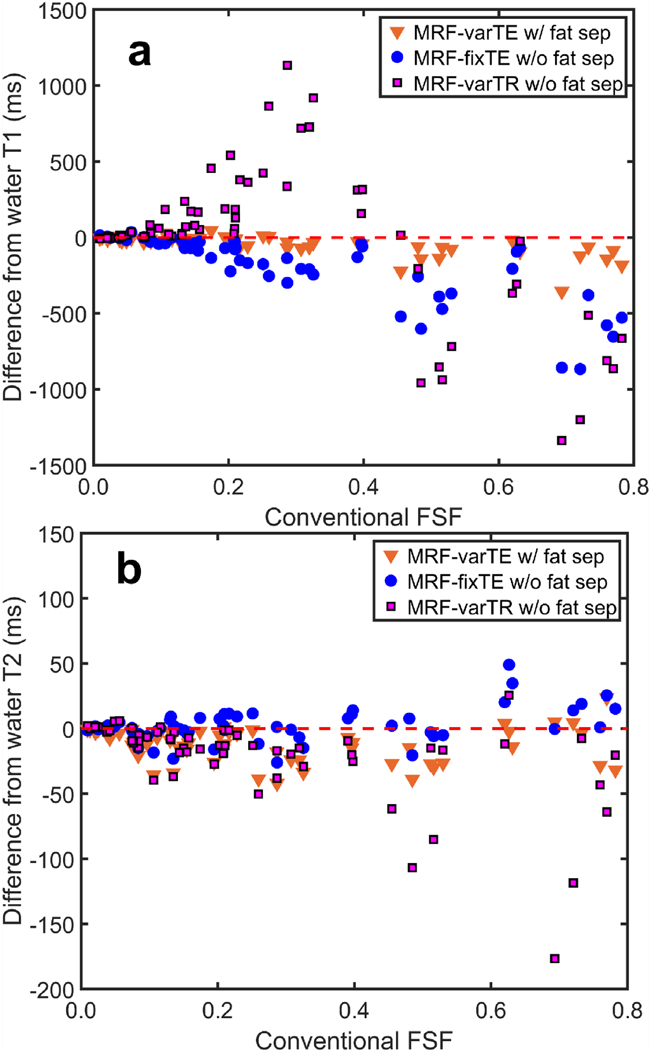
The deviations in MR fingerprinting (MRF) estimated T₁ and T₂ with fat signal fraction (FSF) in the oil-water phantom. The difference from the consensus T₁ estimates for all T₁/T₂ tube combinations and all measured slices is shown for the proposed k-space fat-water separation (MRF-varTE) and fixed-TE/variable-TR MRF methods without fat-water separation, plotted against FSF estimated from a spoiled gradient echo sequence (a). The changes in T₂ versus FSF are plotted in (b).

Figure 6 plots FSF estimates from the proposed MRF method against the SPGR-derived values for all tubes and oil-water slices. Example FSF and B₀ maps are also shown. The FSF maps indicate general agreement between the FSF and graph cut fat-water separation across the phantom tubes. The B₀ maps show perturbations within 100 Hz, with more discretization and lower B₀ estimates in the MRF map relative to the SPGR derived map. The FSF estimates are concordant with CCC = 0.990 across the different tubes with differing T₁ and T₂.

Fig. 6.

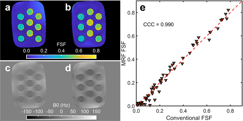
Example fat signal fraction (FSF), B₀ maps and FSF concordance over a large range of T₁/T₂’s from the oil-water phantom. The conventional spoiled gradient echo (SPGR) (a) and proposed MR fingerprinting (MRF) (b) FSF estimates are shown with the estimated SPGR (c) and MRF (d) B₀ maps from the oil-water phantom slice shown in Fig. 4. The FSF concordance between the MRF and SPGR method is plotted in (e) for all measured water/oil-water layers across all T₁/T₂ tube combinations with the concordance correlation coefficient (CCC) displayed.

Figure 7 shows the results from the poorly shimmed condition at an FSF layer of ~10 to 30%. Without B₀ correction, the k-space-based MRF fat-water separation FSF bias is substantial in regions with high B₀ (Fig. 7b). The B₀ estimate from the graph cut processing (Fig. 7d) appears more negative than that from the MRF method. Fat-water swaps are visible at the extreme limbs of the phantom of both methods.

Fig. 7.

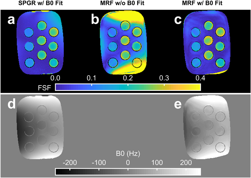
The fat signal fraction (FSF) and B₀ estimate from conventional and MR fingerprinting (MRF) methods. The FSF maps for a single slice in the oil-water phantom with heterogeneous Bo are shown for the reference spoiled gradient echo (SPGR) with graph cut processing (a), the MRF k-space based fat separation method without B₀ correction (b) and the MRF k-space based fat separation method with B₀ correction (c). The estimated SPGR (d) and MRF (e) B₀ maps are also displayed. The data are from the same slice as depicted in Fig. 8.

Figure 8 provides example T₁ and T₂ maps from the well shimmed and poorly shimmed slice, without and with B₀ correction. Without B₀ correction, substantial deviations in T₁ and T₂ are observed in regions of B₀ perturbation. These deviations are reduced by > 100 ms in some cases with the proposed B₀ correction.

Fig. 8.

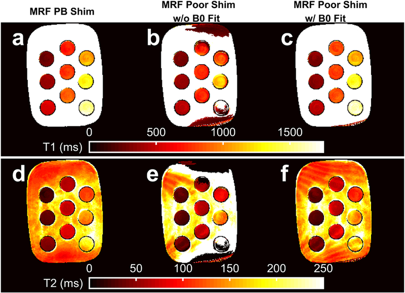
The MR fingerprinting (MRF) estimated T₁ and T₂ maps without and with B₀ correction. Variable TE MRF T₁ and T₂ maps with pencil-beam (PB) shimming (a, d) are shown for comparison with poorly shimmed T₁ and T₂ maps from MRF k-space fat-water separation without B₀ correction (b, e) and k-space fat-water separation with Bo correction (c, f). The data are from the same slice as depicted in Fig. 7.

4.3. In Vivo Studies

Figures 9 and 10 show the FSF, T₁ and T₂ estimates from the knee and brain. The knee FSF estimates between the SPGR and MRF data appear largely consistent (Fig. 9b). Compared to the SPGR measurement, the MRF FSF appears slightly lower in the gastrocnemius and biceps femoris and slightly higher in the subcutaneous and intermuscular fat regions. The fat-suppressed IR-TFE and MSE measurements appear mostly uniform across the main muscle groups visible in the parameter maps (Fig. 9c, d). The MRF T₁s appear lower than the IR-TFE measurements within the main muscle bodies and higher in T₂ than the MSE measurements. The MRF-fixTE and MRF-varTR T₁ and T₂ exhibit bands of lower and higher T₁ and T₂ estimates near the muscle-fat interfaces throughout the FOV. The B₀ and FSF parameter maps from the brain from the proposed method are similar to the SPGR reference maps (Fig. 10). The periorbital fat is clearly defined on the FSF maps, with low FSF in the brain and optic nerve tracts. The conventional and MRF B₀ maps both reveal increases in B₀ superior to the temporal bone. Deviations from the FSF and B₀ maps include fat-water swapping in the anterior orbits and in a small region in the optic nerves, as well as a posterior circular flow artifact. T₁ and T₂ maps in the brain appear similar in all MRF methods except for the orbits, optical nerve, and regions near extracranial fat.

Fig. 9.

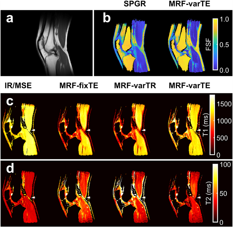
Multi-parametric knee maps. An anatomical reference from T₁-weighted images (a) with fat signal fraction (FSF) maps from spoiled gradient echo (SPGR) and the proposed MR fingerprinting fat-water separation methods (b) are shown. The T1 maps (c) from fat-suppressed inversion recovery (IR-TFE) are shown next to the MRF fixed TE (MRF-fixTE), MRF variable TR (MRF-varTR) without fat-water separation and the proposed method with fat-water separation using MRF variable TE (MRF-varTE). The fat-suppressed multiple spin-echo (MSE) T₂ maps are shown adjacent to the MR-fixTE, MRF-varTR and proposed method acquired with MRF-varTE T₂ estimates (d). Parameter maps were masked using the SPGR derived water image and threshold. Bands of lower T₁ and higher T₂ appear near fat-muscle interfaces in the MRF-fixTE and MRF-varTR parameter maps, which do not account for fat. An arrowhead marks a point on all T₁/T₂ knee parameter maps where there are multiple fat-muscle interfaces and the banding effect is pronounced.

Fig. 10.

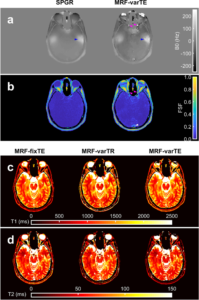
Multi-parametric maps of the brain. The B₀ maps from the spoiled gradient with graph cut processing (SPGR) and the proposed MR fingerprinting (MRF) fat-water and B₀ estimation method with variable TE (MRF-varTE) are shown (a), with the corresponding fat signal fraction maps (b). The MRF method has general agreement with the SPGR. Blue arrows indicate a region superior to the temporal bone featuring increased Bo heterogeneity in both methods, which is also present on the contralateral side (unmarked). Deviations between the methods include fat-water swapping in the anterior orbits and small sections of the optic nerves (magenta arrows), and the MRF FSF map indicates an area of a flow artifact (white arrow). The MRF T1 (c) and T2 maps are shown for the MRF methods without fat-water separation (MRF-fixTE/-varTE) and the proposed fat-water separation using MRF-varTE. The slice thickness (5 mm) is thicker than the optic nerve diameter so may include a partial volume of CSF.

The abdominal MRF data was successfully acquired in a single breath hold and can be seen in Fig. 11. Fine features of visceral, subcutaneous and marrow fat can be visualized in the FSF map. The fat-separated T₁ and T₂ estimates of the liver are 1,093 and 19 ms, respectively. In comparison, 3T MR spectroscopy water relaxometry estimates of the liver from the literature are 990 (SD 89) ms for T₁ and 30 (SD 2) ms for T₂.[58]

Fig. 11.

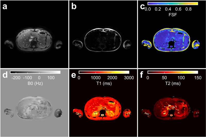
The proposed MR fingerprinting method applied in the abdomen. The water (a) and fat (b) images, and fat signal fraction (FSF) (c), B₀ (d), Ti (e) and T2(f) maps estimated by the proposed technique are shown for a single slice in the liver. Parameter maps (c-f) were masked using the sum of the water (a) and fat (b) magnitude images with a threshold. The MRF and B₁+ acquisitions were separately acquired using end-expiration breath holds.

5. DISCUSSION

The results indicate that small fractions of fat signal significantly bias T₁ and T₂ water estimates from MRF techniques that do not consider fat. The proposed MRF method ameliorates these biases, circumvents spiral blurring, and incorporates a B₀ correction that substantially improves parameter map quality.

The simulation, phantom, and in vivo results all show that fat biases MRF T₁ and T₂ estimation. This bias in T₁ can exceed 200 ms at FSF >0.2 (Figs. 2–5). From the image simulations, the noiseless, fully sampled MRF parameter estimates without fat separation were equally biased as the noisy, undersampled estimates, suggesting that fat signal contamination may in some cases be the dominate form of bias, relative to instrument noise or aliasing. The knee results (Fig. 9) showed that in regions which do not contain fat, bias may be avoided by excluding regions close to fat from analysis. However, fat signal contamination of the T₁ and T₂ estimates may be inescapable if fat is diffusely spread throughout, or immediately adjacent to, the tissue of interest. This is common in nonalcoholic fatty liver disease[59], pancreatic steatosis[60], fat-infiltrating myopathies[4], and pericardial fat[61].

The proposed MRF fat separation method reduces bias of T₁ and T₂ due to fat, relative to the MRF-fixTE and MRF-varTR techniques; it also provides FSF estimates. Figures 3–5 show that the proposed method substantially reduces the bias in T₁, relative to MRF without fat-separation. The MRF-fixTE (in-phase TE) and -varTR (õpposed-phase TE) results likely indicate that in-phase TE reduces T₁ and T₂ bias when fat separation is not used. The FSF CCC of 0.990 between the MRF and SPGR measurements (Fig. 6) includes a broad range of T₁ and T₂ combinations, suggesting that water T₁/T₂ are not biasing the MRF FSF estimate. While high concordance can be achieved with spiral MRF directly estimating FSF with a dictionary matching scheme in the image domain, Supplementary Fig. S8 shows that blurring due to chemical shift may degrade parameter map quality.

The B₀ correction from the proposed technique improves FSF, T₁, and T₂ estimation compared to those estimates made without the correction. MFI approximates the true B₀ correction because of the finite number of basis frequencies and the nonzero gradient of B₀. However, the proposed correction still helps to significantly improve the relaxometry estimates in regions of B₀ > 100 Hz (Figs. 7 and 8) and mostly follows the reference B₀ map in the brain with the noted exceptions (Fig. 10). Figs. 7–8 show that without the proposed B₀ correction, the phase modulation may confound the variable echo time MRF sequence needed to encode fat chemical shift information, as well as confound the T₁ and T₂ estimation using the dictionary that does not contain off-resonance information.

The in vivo data suggest this technique may be applied to improve MRF extracranial relaxometry and FSF measurements. The knee FSF maps (Fig. 9) appear concordant between MRF and conventional techniques in the marrow and intermuscular fat. The MRF T₁/T₂ maps (Fig. 9) indicate bias near fat regions without fat separation, in agreement with the phantom results. While T₂* is not explicitly considered in this work, the spin-spin (T₂) component of T₂* is considered, leaving the refocusable transverse relaxation (T₂’) unmodeled. The in vivo magnitude of this potential bias from T2’ is not clear but can potentially be included in the fitting with modifications to the above theory, which we leave for future work. Nevertheless, the addition of FSF and B₀ estimates to relaxometry increases the amount of information available from a single MRF sequence, supporting its continued study for potential applications in clinical research. The MRF data for fat-separated multi-parametric abdominal study (Fig. 11) were acquired in 24 s with a single breath hold. Future quantitative MRI studies in the extremities, abdomen, thorax or neck may be made more practicable by using the proposed technique.

Limitations of this study include the fixed fat model assumption, regularization of the B₀ fitting, aliasing, independent B₁+ mapping, and the in vivo study size. Allowing an unconstrained fitting for fat T₁ and T₂ and signal amplitude would likely dramatically increase the memory requirements of the solution as well as make the k-space fat-water separation increasingly ill-posed. However, the extent to which any potential variability in in vivo fat relaxation properties quantitatively impact the observed signals is not clear. For instance, inversion recovery-based fat suppression generally assumes a fixed T₁ for fat. A recently described MRF approach to multi-compartment relaxometry [62] could potentially be applied to this problem, but is outside the scope of this work. The image simulations suggest that aliasing contributes to uncertainty: the relaxometry standard deviations are zero for the proposed method when fully-sampled (Supplementary Figs. S6-S7), but are non-zero when aliasing is introduced without any noise (Fig. 3). Incorporation of matrix completion[63] or low-rank[64] reconstruction methods may reduce these uncertainties. The fat-water swapping in Fig. 10 may be reduced by more rigorous incorporation of spatial roughness penalties or other regularization to limit sudden changes in estimated B₀. The MRF scan durations reported in this proof-of-concept study do not include the time required to acquire independent B₁+ mapping. However, methods such as dual refocused echo acquisition mode[57] (Fig. 11) and Bloch-Siegert shift[65] can map B₁+ on the order of seconds and have been previously employed in MRF to this end[41]. Integrating B₁+ mapping into the MRF sequence is an active area of research[66]. The in vivo MRF T₁ and T₂ estimates outside of fatty regions generally agreed with each other in the knee and the brain, but further study with more subjects are needed to understand the difference between MRF with/without fat-separation and conventional techniques in different organs.

In support of reproducible research, the source code along with figure reproduction scripts and data are freely available for download at https://github.com/jostenson/MRI_Ostenson_MRF_FSF (SHA-1: XXX to be determined pending acceptance of the manuscript).

6. CONCLUSIONS

We have developed a means to simultaneously estimate T₁, T₂, and FSF with inline B₀ correction using a single MRF sequence. The method improves T₁ and T₂ estimation in regions of fat over non-fat separating MRF methods and adds to the parameters available for estimation via MRF. This unification of multi-parametric estimation increases the amount of information gathered by the MRF sequence and extends MRF’s possible utility.

References

- [1].Taylor AJ, Salerno M, Dharmakumar R, Jerosch-Herold M. T1 Mapping Basic Techniques and Clinical Applications. JACC Cardiovasc Imaging 2016;9:67–81. doi: 10.1016/j.jcmg.2015.11.005. [DOI] [PubMed] [Google Scholar]
- [2].Giri S, Chung Y-C, Merchant A, Mihai G, Rajagopalan S, Raman SV., et al. T2 quantification for improved detection of myocardial edema. J Cardiovasc Magn Reson 2009;11:56. doi: 10.1186/1532-429X-11-56. [DOI] [PMC free article] [PubMed] [Google Scholar]
- [3].Hoad CL, Palaniyappan N, Kaye P, Chernova Y, James MW, Costigan C, et al. A study of T 1 relaxation time as a measure of liver fibrosis and the influence of confounding histological factors. NMR Biomed 2015;28:706–14. doi: 10.1002/nbm.3299. [DOI] [PubMed] [Google Scholar]
- [4].Arpan I, Forbes SC, Lott DJ, Senesac CR, Daniels MJ, Triplett WT, et al. T2 mapping provides multiple approaches for the characterization of muscle involvement in neuromuscular diseases: A cross-sectional study of lower leg muscles in 5–15-year-old boys with Duchenne muscular dystrophy. NMR Biomed 2013;26:320–8. doi: 10.1002/nbm.2851. [DOI] [PMC free article] [PubMed] [Google Scholar]
- [5].Wei Y, Wu S, Gao F, Sun T, Zheng D, Ning P, et al. Esophageal carcinoma: Ex vivo evaluation by high-spatial-resolution T2 -mapping MRI compared with histopathological findings at 3.0T. J Magn Reson Imaging 2016:1609–16. doi: 10.1002/jmri.25509. [DOI] [PubMed] [Google Scholar]
- [6].Sabouri S, Chang SD, Savdie R, Zhang J, Jones EC, Goldenberg SL, et al. Luminal Water Imaging: A New MR Imaging T2 Mapping Technique for Prostate Cancer Diagnosis. Radiology 2017;284:451–9. doi: 10.1148/radiol.2017161687. [DOI] [PMC free article] [PubMed] [Google Scholar]
- [7].Hu HH, Smith DL, Nayak KS, Goran MI, Nagy TR. Identification of brown adipose tissue in mice with fat-water IDEAL-MRI. J Magn Reson Imaging 2010;31:1195–202. doi: 10.1002/jmri.22162. [DOI] [PMC free article] [PubMed] [Google Scholar]
- [8].Tang A, Tan J, Sun M, Hamilton G, Bydder M, Wolfson T, et al. Nonalcoholic Fatty Liver Disease: MR Imaging of Liver Proton Density Fat Fraction to Assess Hepatic Steatosis. Radiology 2013;267:422–31. doi: 10.1148/radiol.12120896. [DOI] [PMC free article] [PubMed] [Google Scholar]
- [9].Kukuk GM, Hittatiya K, Sprinkart AM, Eggers H, Gieseke J, Block W, et al. Comparison between modified Dixon MRI techniques, MR spectroscopic relaxometry, and different histologic quantification methods in the assessment of hepatic steatosis. Eur Radiol 2015;25:2869–79. doi: 10.1007/s00330-015-3703-6. [DOI] [PubMed] [Google Scholar]
- [10].Pokharel SS, Macura KJ, Kamel IR, Zaheer A. Current MR imaging lipid detection techniques for diagnosis of lesions in the abdomen and pelvis. Radiographics 2013;33:681–702. doi: 10.1148/rg.333125068. [DOI] [PubMed] [Google Scholar]
- [11].Jiang Y, Ma D, Seiberlich N, Gulani V, Griswold MA. MR fingerprinting using fast imaging with steady state precession (FISP) with spiral readout. Magn Reson Med 2015;74:1621–31. doi: 10.1002/mrm.25559. [DOI] [PMC free article] [PubMed] [Google Scholar]
- [12].Chen Y, Jiang Y, Pahwa S, Ma D, Lu L, Twieg MD, et al. MR Fingerprinting for Rapid Quantitative Abdominal Imaging. Radiology 2016;279:278–86. doi: 10.1148/radiol.2016152037. [DOI] [PMC free article] [PubMed] [Google Scholar]
- [13].Yu AC, Badve C, Ponsky LE, Pahwa S, Dastmalchian S, Rogers M, et al. Development of a Combined MR Fingerprinting and Diffusion Examination for Prostate Cancer. Radiology 2017;283:729–38. doi: 10.1148/radiol.2017161599. [DOI] [PMC free article] [PubMed] [Google Scholar]
- [14].Hamilton JI, Jiang Y, Chen Y, Ma D, Lo W-C, Griswold M, et al. MR fingerprinting for rapid quantification of myocardial T 1, T 2, and proton spin density. Magn Reson Med 2017;77:1446–58. doi: 10.1002/mrm.26216. [DOI] [PMC free article] [PubMed] [Google Scholar]
- [15].Hamilton G, Smith DL, Bydder M, Nayak KS, Hu HH. MR properties of brown and white adipose tissues. J Magn Reson Imaging 2011;34:468–73. doi: 10.1002/jmri.22623. [DOI] [PMC free article] [PubMed] [Google Scholar]
- [16].Bojorquez JZ, Bricq S, Acquitter C, Brunotte F, Walker PM, Lalande A. What are normal relaxation times of tissues at 3 T? Magn Reson Imaging 2017;35:69–80. doi: 10.1016/j.mri.2016.08.021. [DOI] [PubMed] [Google Scholar]
- [17].Rakow-Penner R, Daniel B, Yu H, Sawyer-Glover A, Glover GH. Relaxation times of breast tissue at 1.5T and 3T measured using IDEAL. J Magn Reson Imaging 2006;23:87–91. doi: 10.1002/jmri.20469. [DOI] [PubMed] [Google Scholar]
- [18].Mozes FE, Tunnicliffe EM, Pavlides M, Robson MD. Influence of fat on liver T1 measurements using modified Look-Locker inversion recovery (MOLLI) methods at 3T. J Magn Reson Imaging 2016;44:105–11. doi: 10.1002/jmri.25146. [DOI] [PMC free article] [PubMed] [Google Scholar]
- [19].Del Grande F, Santini F, Herzka DA, Aro MR, Dean CW, Gold GE, et al. Fat-suppression techniques for 3-T MR imaging of the musculoskeletal system. Radiographics 2014;34:217–33. doi: 10.1148/rg.341135130. [DOI] [PMC free article] [PubMed] [Google Scholar]
- [20].Hernando D, Haldar JP, Sutton BP, Ma J, Kellman P, Liang ZP. Joint estimation of water/fat images and field inhomogeneity map. Magn Reson Med 2008;59:571–80. doi: 10.1002/mrm.21522. [DOI] [PMC free article] [PubMed] [Google Scholar]
- [21].Reeder SB, Wen Z, Yu H, Pineda AR, Gold GE, Markl M, et al. Multicoil Dixon Chemical Species Separation with an Iterative Least-Squares Estimation Method. Magn Reson Med 2004;51:35–45. doi: 10.1002/mrm.10675. [DOI] [PubMed] [Google Scholar]
- [22].Hernando D, Kellman P, Haldar JP, Liang ZP. Robust water/fat separation in the presence of large field inhomogeneities using a graph cut algorithm. Magn Reson Med 2010;63:79–90. doi: 10.1002/mrm.22177. [DOI] [PMC free article] [PubMed] [Google Scholar]
- [23].Doneva M, Börnert P, Eggers H, Mertins A, Pauly J, Lustig M. Compressed sensing for chemical shift-based water-fat separation. Magn Reson Med 2010;64:1749–59. doi: 10.1002/mrm.22563. [DOI] [PubMed] [Google Scholar]
- [24].Ma D, Gulani V, Seiberlich N, Liu K, Sunshine JL, Duerk JL, et al. Magnetic resonance fingerprinting. Nature 2013;495:187–92. doi: 10.1038/nature11971. [DOI] [PMC free article] [PubMed] [Google Scholar]
- [25].Cloos MA, Knoll F, Zhao T, Block KT, Bruno M, Wiggins GC, et al. Multiparametric imaging with heterogeneous radiofrequency fields. Nat Commun 2016;7:12445. doi: 10.1038/ncomms12445. [DOI] [PMC free article] [PubMed] [Google Scholar]
- [26].Han D, Kim M-O, Lee H, Hong T, Kim D-H. A Free-breathing water/fat separation and T1, T2 quantification method using dual TR FISP in abdomen. Proc Intl Soc Mag Reson Med, 2016, p. 0575. [Google Scholar]
- [27].Ostenson J, Welch EB. Fat Signal Fraction Determination Using MR Fingerprinting. Proc Intl Soc Mag Reson Med, 2017, p. 0134. [Google Scholar]
- [28].Cencici M, Biagi L, Kaggie J, Schulte RF, Rosetti MT, Buonincontri G. MR Fingerprinting in the knee with dictionary-based fat and water separation. ISMRM Work. MRF, 2017. [DOI] [PMC free article] [PubMed] [Google Scholar]
- [29].Nolte T, Truhn D, Gross-Weege N, Doneva M, Koken P, Elevelt A, et al. Undersampled Spiral Magnetic Resonance Fingerprinting with Water and Fat Blurring Correction. Proc. 26th Annu. Meet ISMRM, 2018, p. 4215. [Google Scholar]
- [30].Koolstra K, Webb A, Koken P, Nehrke K, Börnert P. Water-Fat Separation in Spiral Magnetic Resonance Fingerprinting using Conjugate Phase Reconstruction. Proc. 26th Annu. Meet ISMRM, 2018, p. 0681. [Google Scholar]
- [31].Tosetti M, Buonincontri G, Cencini M, Biagi L, Kaggie JD, Schulte RF. Magnetic resonance fingerprinting with dictionary - based fat and water separation (DBFW MRF ): A multi - component approach 2018. doi: 10.1002/mrm.27628. [DOI] [PMC free article] [PubMed] [Google Scholar]
- [32].Wang D, Zwart NR, Pipe JG. Joint water-fat separation and deblurring for spiral imaging. Magn Reson Med 2017;00:1–11. doi: 10.1002/mrm.26950. [DOI] [PubMed] [Google Scholar]
- [33].Man LC, Pauly JM, Macovski A. Multifrequency interpolation for fast off-resonance correction. Magn Reson Med 1997;37:785–92. [DOI] [PubMed] [Google Scholar]
- [34].Ostenson J, Robison RK, Zwart NR, Welch EB. Multi-frequency interpolation in spiral magnetic resonance fingerprinting for correction of off-resonance blurring. Magn Reson Imaging 2017;41:63–72. doi: 10.1016/j.mri.2017.07.004. [DOI] [PMC free article] [PubMed] [Google Scholar]
- [35].Brodsky EK, Holmes JH, Yu H, Reeder SB. Generalized k-space decomposition with chemical shift correction for non-Cartesian water-fat imaging. Magn Reson Med 2008;59:1151–64. doi: 10.1002/mrm.21580. [DOI] [PubMed] [Google Scholar]
- [36].McGivney DF, Pierre E, Ma D, Jiang Y, Saybasili H, Gulani V, et al. SVD compression for magnetic resonance fingerprinting in the time domain. IEEE Trans Med Imaging 2014;33:2311–22. doi: 10.1109/TMI.2014.2337321. [DOI] [PMC free article] [PubMed] [Google Scholar]
- [37].Bernstein MA, King KF, Zhou XJ. Handbook of MRI Pulse Sequences. Academic Press; 2004. [Google Scholar]
- [38].Flassbeck S, Schmidt S, Breithaupt M, Bachert P, Ladd ME, Schmitter S. On the In fl uence of Intra-Voxel Dephasing in FISP-MRF with Variable Repetition Time. Proc Intl Soc Mag Reson Med 2017:1492. [Google Scholar]
- [39].Schomberg H Off-resonance correction of MR images. IEEE Trans Med Imaging 1999;18:481–95. doi: 10.1109/42.781014. [DOI] [PubMed] [Google Scholar]
- [40].Eggers H, Knopp T, Potts D. Field inhomogeneity correction based on gridding reconstruction for magnetic resonance imaging. IEEE Trans Med Imaging 2007;26:374–84. doi: 10.1109/TMI.2006.891502. [DOI] [PubMed] [Google Scholar]
- [41].Ma D, Coppo S, Chen Y, Mcgivney DF, Jiang Y, Pahwa S, et al. Slice Profile and B 1 Corrections in 2D Magnetic Resonance Fingerprinting. Magn Reson Med 2017;00:1–9. doi: 10.1002/mrm.26580. [DOI] [PMC free article] [PubMed] [Google Scholar]
- [42].Pipe JG, Zwart NR. Spiral trajectory design: A flexible numerical algorithm and base analytical equations. Magn Reson Med 2014;71:278–85. doi: 10.1002/mrm.24675. [DOI] [PubMed] [Google Scholar]
- [43].Zwart NR, Johnson KO, Pipe JG. Efficient sample density estimation by combining gridding and an optimized kernel. Magn Reson Med 2012;67:701–10. doi: 10.1002/mrm.23041. [DOI] [PubMed] [Google Scholar]
- [44].Uecker M, Lai P, Murphy MJ, Virtue P, Elad M, Pauly JM, et al. ESPIRiT - An eigenvalue approach to autocalibrating parallel MRI: Where SENSE meets GRAPPA. Magn Reson Med 2014;71:990–1001. doi: 10.1002/mrm.24751. [DOI] [PMC free article] [PubMed] [Google Scholar]
- [45].Uecker M, Tamir JI. BART: version 0.4.02 (Version v0.4.02) 2017. doi: 10.5281/zenodo.1066014. [DOI]
- [46].Welch EB, Robison RK, Harkins KD. Robust k-space trajectory mapping with data readout concatenation and automated phase unwrapping reference point identi cation. Proc Intl Soc Mag Reson Med, 2017, p. 1387. [Google Scholar]
- [47].Duyn JH, Yang Y, Frank JA, van der Veen JW. Simple correction method for k-space trajectory deviations in MRI. J Magn Reson 1998;132:150–3. doi: 10.1006/jmre.1998.1396. [DOI] [PubMed] [Google Scholar]
- [48].Weigel M Extended phase graphs: Dephasing, RF pulses, and echoes - Pure and simple. J Magn Reson Imaging 2015;41:266–95. doi: 10.1002/jmri.24619. [DOI] [PubMed] [Google Scholar]
- [49].Jiang Y, Ma D, Keenan KE, Stupic KF, Gulani V, Griswold MA. Repeatability of magnetic resonance fingerprinting T 1 and T 2 estimates assessed using the ISMRM/NIST MRI system phantom. Magn Reson Med 2017;78:1452–7. doi: 10.1002/mrm.26509. [DOI] [PMC free article] [PubMed] [Google Scholar]
- [50].Yarnykh VL. Actual flip-angle imaging in the pulsed steady state: a method for rapid three-dimensional mapping of the transmitted radiofrequency field. Magn Reson Med 2007;57:192–200. doi: 10.1002/mrm.21120. [DOI] [PubMed] [Google Scholar]
- [51].Zhao B, Haldar JP, Liao C, Ma D, Jiang Y, Griswold MA, et al. Optimal Experiment Design for Magnetic Resonance Fingerprinting: Cramér-Rao Bound Meets Spin Dynamics. IEEE Trans Med Imaging 2018;PP:1–1. doi: 10.1109/TMI.2018.2873704. [DOI] [PMC free article] [PubMed] [Google Scholar]
- [52].Fessler JA, Sutton BP. Nonuniform fast fourier transforms using min-max interpolation. IEEE Trans Signal Process 2003;51:560–74. doi: 10.1109/TSP.2002.807005. [DOI] [Google Scholar]
- [53].Crawford SB, Kosinski AS, Lin HM, Williamson JM, Barnhart HX. Computer programs for the concordance correlation coefficient. Comput Methods Programs Biomed 2007;88:62–74. doi: 10.1016/j.cmpb.2007.07.003. [DOI] [PubMed] [Google Scholar]
- [54].Poon CS, Henkelman RM. 180° Refocusing Pulses Which Are Insensitive To Static and Radiofrequency Field Inhomogeneity. J Magn Reson 1992;99:45–55. doi: 10.1016/0022-2364(92)90154-Y. [DOI] [Google Scholar]
- [55].Li K, Zu Z, Xu J, Janve VA, Gore JC, Does MD, et al. Optimized inversion recovery sequences for quantitative T1 and magnetization transfer imaging. Magn Reson Med 2010;64:491–500. doi: 10.1002/mrm.22440. [DOI] [PMC free article] [PubMed] [Google Scholar]
- [56].Otsu N A Threshold Selection Method from Gray-Level Histograms. IEEE Trans Syst Man Cybern 1979;9:62–6. doi: 10.1109/TSMC.1979.4310076. [DOI] [Google Scholar]
- [57].Nehrke K, Börnert P. DREAM-a novel approach for robust, ultrafast, multislice B1 mapping. Magn Reson Med 2012;68:1517–26. doi: 10.1002/mrm.24158. [DOI] [PubMed] [Google Scholar]
- [58].Weis J, Kullberg J, Ahlström H. Multiple breath-hold proton spectroscopy of human liver at 3T: Relaxation times and concentrations of glycogen, choline, and lipids. J Magn Reson Imaging 2018;47:410–7. doi: 10.1002/jmri.25734. [DOI] [PubMed] [Google Scholar]
- [59].Brunt EM, Tiniakos DG. Histopathology of nonalcoholic fatty liver disease. World J Gastroenterol 2010;16:5286–96. doi: 10.3748/wjg.v16.142.5286. [DOI] [PMC free article] [PubMed] [Google Scholar]
- [60].Smits MM, van Geenen EJM. The clinical significance of pancreatic steatosis. Nat Rev Gastroenterol Hepatol 2011;8:169–77. doi: 10.1038/nrgastro.2011.4. [DOI] [PubMed] [Google Scholar]
- [61].Wong CX, Abed HS, Molaee P, Nelson AJ, Brooks AG, Sharma G, et al. Pericardial fat is associated with atrial fibrillation severity and ablation outcome. J Am Coll Cardiol 2011;57:1745–51. doi: 10.1016/j.jacc.2010.11.045. [DOI] [PubMed] [Google Scholar]
- [62].McGivney D, Deshmane A, Jiang Y, Ma D, Badve C, Sloan A, et al. Bayesian estimation of multicomponent relaxation parameters in magnetic resonance fingerprinting. Magn Reson Med 2018;80:159–70. doi: 10.1002/mrm.27017. [DOI] [PMC free article] [PubMed] [Google Scholar]
- [63].Doneva M, Amthor T, Koken P, Sommer K, Börnert P. Matrix completion-based reconstruction for undersampled magnetic resonance fingerprinting data. Magn Reson Imaging 2017;41:41–52. doi: 10.1016/j.mri.2017.02.007. [DOI] [PubMed] [Google Scholar]
- [64].Zhao B, Setsompop K, Adalsteinsson E, Gagoski B, Ye H, Ma D, et al. Improved magnetic resonance fingerprinting reconstruction with low-rank and subspace modeling. Magn Reson Med 2018;79:933–42. doi: 10.1002/mrm.26701. [DOI] [PMC free article] [PubMed] [Google Scholar]
- [65].Sacolick LI, Wiesinger F, Hancu I, Vogel MW. B1 mapping by Bloch-Siegert shift. Magn Reson Med 2010;63:1315–22. doi: 10.1002/mrm.22357. [DOI] [PMC free article] [PubMed] [Google Scholar]
- [66].Buonincontri G, Schulte RF, Cosottini M, Tosetti M. Spiral MR fingerprinting at 7 T with simultaneous B1 estimation. Magn Reson Imaging 2017;41:1–6. doi: 10.1016/j.mri.2017.04.003. [DOI] [PubMed] [Google Scholar]
Associated Data
This section collects any data citations, data availability statements, or supplementary materials included in this article.