

Abstract
The monitoring of rotating machinery condition has been a critical component of the Industry 4.0 revolution in enhancing machine reliability and facilitating intelligent manufacturing. The introduction of condition-based monitoring has effectively reduced the catastrophic events and maintenance cost across various industries. One of the major challenges of the diagnosis remains as majority of the diagnostic model requires off-line analysis and human intervention. The offline analysis, which is normally done by previous experience, involves tuning model parameters to improve the performance of the diagnostic model. However, for newly developed models, the knowledge of the unknown parameters does not exist. One way to resolve this issue is through learning using adaptation. The adaptation algorithm adjusts itself by newly acquired data. Hence, improvement of the model performance is achieved. In this paper, a nonlinear adaptive dictionary learning algorithm is proposed to achieve early fault detection of bearing elements without using the conventional computation heavy algorithm to update the dictionary. Deterministic and random data separation is implemented using the autoregressive model to reduce the background noise. The filtered data is further analyzed by the Infogram to reveal the impulsiveness and cyclostationary signature of the vibration signal. The dictionary is initialized using random parameters. Instead of using the k means singular value decomposition algorithm to compute the dictionary for adaptation, the unscented Kalman filter (UKF) is implemented to update the dictionaries using the filtered signal from the Infogram. The updating algorithm does not require computation of the dictionary, and no previous knowledge of the dictionary’s parameters is needed. The updated dictionary contains the detected fault signature from the Infogram and, therefore, is used for further fault analysis. The proposed algorithm has the advantage of self-adaptation, the capability to map the non-linear relationship of the signal and dictionary weights. The algorithm can be used in the various condition-based monitoring of rotating machineries to avoid additional human efforts and improve the performance of the diagnostic model.
Keywords: Ball bearing, Fault diagnosis, Dictionary learning, Adaptive algorithm
1. Introduction
The continuous safe operation of the rotating machinery relies on the accurate knowledge of the machine health condition [1]. A significant amount of research effort has been invested into the monitoring of the health condition of rotating machinery in the recent years [2–5]. The failure of rotating machinery is normally attributed to the bearing failure, the gear failure, rotating shaft fatigue, and the combination of these failure modes [6]. The inappropriate operation, severe operating condition, and inaccurate knowledge of the proper maintenance interval account for the major reasons that contribute to the catastrophic failure of the machines. The concept of condition-based maintenance or predictive maintenance has been proposed over a few decades [7]. It is still considered the most effective maintenance strategies until now as more effective diagnosis and prognosis techniques are developed [8–12]. The vibration analysis of the vibration signal of bearings accounts for the majority of the current research conducted nowadays.
Randall and Antoni have proposed a general guideline for bearing diagnosis in [2]. A strong background noise signals generated by machine components and data transmission are observed [13]. Therefore, the need of separation of the useful bearing vibration signal and noisy signal cannot be over emphasized. Various techniques are implemented to isolate the system noise and extract the critical information. The preprocessing is generally implemented using the tools of the following categories: order tracking, time synchronous averaging, linear prediction, adaptive noise cancelation, and deterministic/random signal separation [14]. The order tracking method generally requires information of the rotating shaft speed [15]. The vibration data is resampled based on the constant angular increments. The early documented research requires the angular increments to be relatively small to perform the order tracking [16]. The most recent research focuses on large-angle variation and tacholess order tracking [17]. However, the technique requires complex computation algorithm to achieve a relative accurate result. The time synchronous averaging method, in general, requires the tachometer signal [18]. Although method without speed sensor exists [19], the no knowledge exists for effectively choosing angular resampling techniques. Trial and error methods are widely used, and the resampling techniques cannot be generalized [20]. Linear prediction is a relatively attractive way to obtain the deterministic part of the fault signal because of its simplicity [21]. The difficulty of implementation exists in the selection of an appropriate time series model and model order [22, 23]. The adaptive noise cancelation techniques are implemented to separate a signal containing two uncorrelated components such as gear fault and bearing fault [24]. It generally requires a reference signal such as a known faulty gear vibration signal to successfully separate the mixture of signals. For the cases of system background noise and transmission error, the reference input of the model is difficult to determine. The discrete/random separation method does not require adaptation as the adaptive method. However, it requires the frequency components to be stable. In addition, the transfer function between signal and a delayed version of signal needs to be computed, and the transfer function is sensitive to the signal-to-noise ratio [24]. In this paper, the linear prediction method is implemented for the preprocessing of signal because of its simplicity and effectiveness for online monitoring applications.
The most widely implemented signal processing technique for the analysis of bearings’ vibration is the time-frequency domain analysis. The short-time Fourier transform, which uses a moving data window to perform Fourier transform, is the simplest to implement [24]. However, the resolution of the frequency domain signal is dependent on the selection of window size. The wavelet analysis is another popular and efficient way to perform time frequency analysis. A wide variety of the wavelet techniques exists such as the traditional wavelet transform [25], wavelet packet transform [26], and complex wavelet transform [27]. Qiu et al. implemented the wavelet filter in the detection of weak fault signature of rolling element bearings [8]. The wavelet parameter is the key for early fault detection. However, no detailed guideline exists for the selection of the parameters. The most recent research focuses on implemented intelligent algorithm to optimize the wavelet parameter [28]. A comprehensive review of the applications of the wavelet transform can be found in [29]. The Kurtogram [30] has become increasingly popular in the past few years for the analysis of bearing vibration signal because of its high accuracy, ease of implementation, and wide range of applicability. The Kurtogram first uses filter banks to break down the signal into different frequency domains. Then, the kurtosis of the complex envelope of the filtered signal is calculated. The maximum kurtosis value is located, and the corresponding filtered signal is used for further analysis. A large value of the Kurtogram implies more impulsiveness in the signal to be analyzed. However, the Kurtogram has limitation of inability to reveal the cyclostationary characteristics of the signal [31]. This deficiency leads to the development of the Infogram which replaced the kurtosis with negentropy to reveal both the impulsive and cyclostationary characteristics of the vibration signal. This paper implemented the Infogram as a part of the preprocessing tool to acquire the signal to update the dictionary.
The dictionary learning [32] is a powerful artificial intelligent tool for signal feature recognition and feature extraction. The technique is initially developed to analyze multidimensional data [33] for image recovery and denoising. The initiation of the dictionary learning requires calculations of the dictionary. Over the years, various technologies are developed to compute the dictionary and find the sparse representation of the signal to be analyzed [34–36]. Aharon et al. present the k means singular value decomposition (K-SVD) method to compute the dictionaries based on the training data [35]. Later, various modifications have been made to the K-SVD algorithm to improve the computation efficiency [37–39]. After the computation of the dictionaries, a sparse representation of the target signal needed to be obtained. The sparsity of the signal is achieved by the implementation of the orthogonal matching pursuit (OMP) algorithm [40]. Similar to the K-SVD, the OMP algorithm has a wide variety of variations listed in [40–43] to ease computation effort. As mentioned in [35], a possible way to improve the training of the dictionary is assigning weights to the different dictionary. In this case, the weights of the dictionaries can be adjusted by adaptive algorithm and possibly achieve structural adaptation of the dictionaries by eliminating the dictionaries with small weights.
In this paper, a nonlinear adaptive dictionary learning algorithm for bearing signal fault diagnosis is proposed. Instead of using the traditional K-SVD method to train the dictionary for multiple times, the unscented Kalman filter (UKF) is implemented to achieve the adaptation of the dictionary. A nonlinear relationship between the dictionary and the artificial kurtosis is established to achieve the self-adaptation. Compared to the previous documented research, the proposed work does not require the learning of the dictionaries, is free from assumptions on the shift-invariant property, and allows online update for newly collected signals. The model utilizes the AR linear predictor to achieve random signal separation. The Infogram and envelope analysis are implemented to locate the fault frequency band and acquire the training data for the dictionaries. The dictionaries are initialized using a set of random variables and updated using the UKF. A sparse representation of the frequency domain signal is obtained in the end to reveal the fault signatures.
2. Diagnostic model
The proposed adaptive bearing diagnostic model is shown in Fig. 1. The training vibration signal of the bearing is preprocessed by the AR linear predictor to reduce the system noise. The AR model order is selected by trial and error. The autocorrelation function and partial autocorrelation function are obtained to facilitate the AR order selection. The wavelet packet transform is implemented to dyadically decomposing the filtered signal. The square envelope (SE) and square envelope spectrum (SES) of the signal are obtained, and the negentropy of the signal is calculated. The band-passed signal with the maximum negentropy is selected as the training data for the dictionary. The UKF takes the weights of the dictionaries and the artificially created kurtosis as input, and calculates the updated weights of the dictionary. The updated dictionaries are tested using a set of vibration signal with weak fault to validate the diagnostic model.
Fig. 1.

Adaptive bearing diagnostic model
2.1. Infogram
The Infogram is a very similar concept to the Kurtogram with the introduction of the concept of entropy borrowed from thermodynamics. It aims to compensate for the lack of detectability of cyclostationary signal of the Kurtogram. The signal transient is perceived as a deviation from the equilibrium state of the squared envelope, and the cyclic characteristics introduce perturbation in the squared envelope spectrum. Based on the observation from thermodynamics, the concept of negentropy is proposed by Antoni [31] to locate the frequency band that contains the most useful information. The implementation of the Infogram is based on the assumption that the vibration signal of bearings can be separated as shown in (1):
| (1) |
where y(t) is the measured vibration signal, x(t) is the fault signal with impulsiveness and cyclostationarity, and n(t) is the system noise. The instantaneous flow of energy in the selected frequency band is represented by the SE as (2) [31]:
| (2) |
where is the vibration signal of the bearing at the corresponding frequency band, n is the length of the signal, and f is the center frequency of the bandpass filter. The average value of the energy fluctuation is represented by (3) [31]:
| (3) |
where L is the length of the signal after the bandpass filterbank created by wavelet packet transform. The strength of the energy fluctuation can be represented by the variance of the energy flow which is (4) [31]:
| (4) |
When the system has reached equilibrium, the value of the variance equals to 1, and a non-stationary signal will result in a variance value larger than 1. The connection of non-stationarity and nonlinearity for a zero-mean signal can be related to the spectral kurtosis shown in (5):
| (5) |
The spectral kurtosis is reported to be able to account for a single or a few transients in [31]; however, the impact generated by the bearing defect results in multiple repetition of the transient. The discrete Fourier transform of the square envelope signal, also known as the square envelope spectrum, is shown to be effective in transient detection [44]. The square envelope spectrum is denoted as (6) for discrete signal:
| (6) |
where α is the frequency and Fs is the sampling frequency. With the addition of the square envelope spectrum, the Infogram is capable of processing impulsive and cyclostationary signal at the same time.
The negentropy, in replacement of the kurtosis, is calculated as (7) and (8) for the SE and SES signal [45]:
| (7) |
| (8) |
The frequency band with the maximum negentropy is selected as the training data for the dictionary learning.
2.2. Dictionary learning
Dictionary learning as a recent popular tool decomposes a multidimensional signal as a linear combination of k interpretable vectors and compresses the signal in a sparse representation. The collection of such k vectors is referred to a dictionary, and each vector in a dictionary is called an atom. The dictionary learning considers a series of n-dimensional input signal and optimizes a certain loss function to get an over-complete dictionary and the corresponding coefficients . By introducing a sparse regularization term in the loss function, we put a sparsity constraint on the coefficient so that the is a sparse representation of the input signal. The sparsest representation is to apply l0 norm regularization in the loss function,
| (9) |
where m is the number of input signals with i = 1, …, m, and the regularization parameter ρ is a trade-off between the sparsity of xi and the goodness-of-fit, which is specified by the user. D represents the dictionaries to recover the signal. Solving the l0 norm regularization is known to be NP hard, which is not solvable for highdimensional case, i.e., k is large. As others, the relaxation approaches that use l1 norm regularization in the loss function are also widely adapted:
| (10) |
which is also known as Lasso or basis pursuit. The regularization parameter is specified to a value which requires relatively low sparsity while preserving the accuracy of the signal reconstruction. The dictionary learning algorithms aim at finding the sparse representation coefficients and the dictionary alternatively by solving the optimization problem defined in (9) or equivalently:
| (11) |
where d is the targeted sparsity that is equivalent to ρ [42]. More specifically, the algorithm consists of two alternating steps: (1) given current estimation of dictionary, finding the sparse representation coefficient x by solving the regularized least squares problem using method such as the OMP introduced in the next section and (2) updating dictionary atom-wise to optimize the target function defined in (11) for each atom individually, which results in a rank-one approximation problem:
| (12) |
where E is the error between input signal matrix and current recovered signal matrix, a is the updated atom, and bT is the corresponding row of new coefficients in x. The rank-one approximation problem can be either solved by iterative updated method such as gradient descent or Newton methods [46] or by direct solver such as singular value decomposition (SVD) [47].
2.3. Orthogonal matching pursuit
Given an m × n data matrix y and the m × k dictionary matrix D as input, the orthogonal matching pursuit (OMP) algorithm computes k × n sparse representation coefficient matrix x with desired sparsity level of d. The estimate for the recovered signal is Dx, and the residuals are defined by e = y − Dx. As an iterative greedy algorithm, the OMP selects at each step the atom that is most correlated with the current residuals. The OMP updates the residuals by projecting the signal y onto the space spanned by the selected atoms. In particular, the OMP for signal recovery can be summarized as follows:
Initialize the residual as e0 = y, an active set Λp containing p elements from {1, …, k}, and set and counter for iteration as t = 1.
- Find the atom that solves the optimization problem:
and add the atom to the set of selected atoms in Dt.(13) Update and .
- Update the signal estimation through the least square optimization:
(14) - Calculate the new approximation of the data at and the new residual as follows:
(15)
which is the projection onto the linear space spanned by the active atoms.(16) Set t = t + 1 and return to Step 2 until t < p.
Note that the estimate Dy has nonzero indices at the active set , where the estimation in component jt is equals the ith component of .
2.4. Dictionary update using UKF
With observed signal y and sparse representation coefficient x obtained by OMP, we propose an innovative dictionary update algorithm, based on artificially created kurtosis, which enables online application without human intervention. More specifically, instead of calculating dictionary as shown in (12) using computationally intensive algorithm, the dictionary is updated using the UKF proposed by Julier and Uhlman [48]. The UKF uses a third-order polynomial to account for the nonlinearity versus the traditional extended Kalman filter (EKF) which uses first-order approximation. The basic framework for the UKF is similar to the EKF which consists of estimation of the state of a nonlinear system [49]:
| (17) |
| (18) |
where θk denotes the intermediate unobserved state of the system, yk is the observed signal, vk is the process noise which drives the dynamic system, and nk is the observation noise. The parameter estimation is achieved by assuming a nonlinear mapping as (19):
| (19) |
where θk is the input, yk is the output, and the nonlinear function G is parameterized by the weight w. The error ek is defined by (20):
| (20) |
where dk is the desired output. The goal is to solve parameter w which minimizes the square error.
The unscented transformation assumes θ (dimension L) has a mean value of and covariance Px. To obtain the statistics of the observed signal y, a matrix of 2L + 1 sigma vector χi is formed according to the following conditions:
| (21) |
| (22) |
| (23) |
| (24) |
| (25) |
| (26) |
where the scaling factor λ is defined in (27):
| (27) |
in which α determines the spread of the sigma points around the mean . It usually has a relatively small value such as 0.001. κ is known as a secondary scaling parameter which is normally 0, and β is used to embed prior information of the distribution of θ. The sigma vectors are propagated through the nonlinear function defined as:
| (28) |
The mean and covariance for y are estimated using a weighted sample mean and covariance of the posterior sigma points as:
| (29) |
| (30) |
The UKF is an extension of the UT to recursive estimate:
| (31) |
The ith dictionary is updated according to (32):
| (32) |
In this paper, the artifical kurtosis is created using a linear function. Random weights generated by a normal random number generator with mean value of 0 and standard deviation of 1 are assigned to each dictionary. The artifical kurtosis is treated as observation data, and θk is assigned as the actual state similar to [50].
3. Simulation and experiment result
To validate the proposed diagnostic method, the Infogram is first tested by a set of simulated signal from [28]. The AR filter length is set as 30 in this case. The resonance frequency is 3000 Hz, and the fault frequency is 100 Hz. The sampling frequency of the signal is set to be 12,000 Hz. The time domain representation of the simulated signal is shown in Fig. 2, and the AR filtered signal is shown in Fig. 3. The Hilbert transform of the filtered simulated signal is shown in Fig. 4. It can be observed from Fig. 3 that the Hilbert transform does not indicate the right fault frequency. The Infogram in (7) and (8) is performed on the simulated data, and the SE and SES negentropy plots are shown in Figs. 5 and 6. The center frequency for Fig. 5 is calculated to be 3000 Hz which corresponds to the resonance frequency, and the fault frequency and its harmonics are revealed in Fig. 5b in comparison to the one in Fig. 4.
Fig. 2.

Simulated signal of bearing vibration
Fig 3.

AR filtered signal
Fig. 4.

Hilbert transform of the simulated signal
Fig. 5.
a Infogram for SE. b Frequency domain of the filtered signal by the SE Infogram
Fig. 6.

a Infogram for SES. b Frequency domain of the filtered signal by the SES Infogram
The SES Infogram shown in Fig. 6 has a center frequency of 2500 Hz, and the maximum negentropy value occurs at level of 2.5. The corresponding frequency plot also indicates the fault frequency of 100 Hz and its harmonics.
The experimental data from Qiu et al. [8] is used to validate the Infogram and the nonlinear adaptive dictionary learning. The experiment consists of a run-to-failure test as shown in Fig. 7 with four Rexnord ZA-2115 double row bearings mounted on the output shaft rotating at 2000 rpm. A 6000 lbs radial load is applied to the shaft and bearing through a spring mechanism as shown in the experimental setup. The debris in the lubricant is collected through a magnetic plug. Once the accumulated debris exceeds the preset value, the test will terminate. The data acquisition system records every 10 min for the vibration signal and the sampling frequency is 20,480 Hz. The tested bearing had experienced outer race failure by the end of the test. The outer race failure frequency is calculated to be 236.4 Hz.
Fig. 7.

Experimental setup for monitoring of bearing vibration [8]
The training vibration signal acquired in between 5000 min and 5010 min as shown in Fig. 8 is used for the dictionary training.
Fig. 8.

Vibration signal of bearing run-to-failure test
To properly determine the order of the AR filter, the autocorrelation and partial autocorrelation [51] are computed for lag value up to 500 as shown in Figs. 9 and 10. Based on the information obtained from the autocorrelation and partial autocorrelation, the proper estimation model should be anti-persistent. However, the anti-persistent series generally need the fractional ARIMA model, which significantly increases the computation complexity, to have relatively good prediction result. To reduce the computation time and simplify the linear prediction model, the AIC and BIC criteria are implemented instead of the autocorrelation function for multiple AR, ARMA, and ARIMA models to select the best model order. The AR model with an order of 30 is tested to have the lowest AIC and BIC values, which indicates the best fit. The filtered signal is shown in Fig. 11.
Fig. 9.

Autocorrelation of vibration signal
Fig. 10.
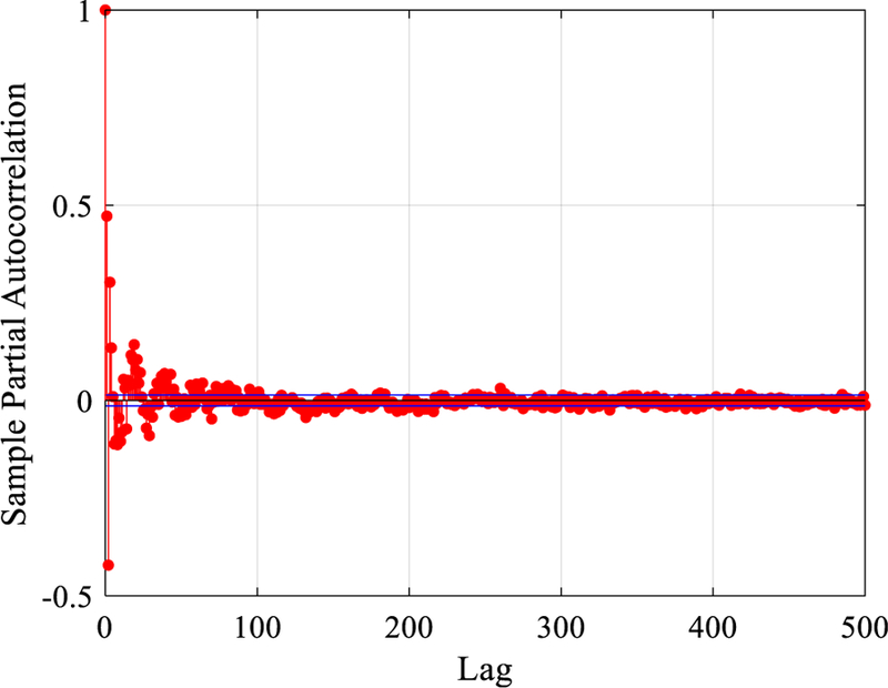
Partial autocorrelation of vibration signal
Fig. 11.

AR filtered vibration signal
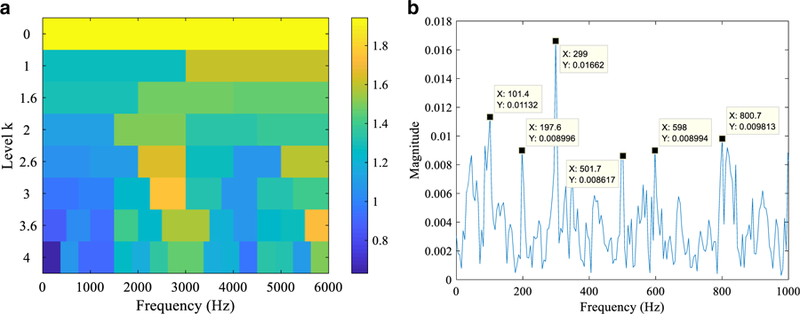
The signal is analyzed by the Infogram using the wave-let packet transform as the filter bank, and the SE and SES Infogram are shown in Figs. 12 and 13 respectively. The SE Infogram indicates a center frequency of 5120 Hz, and the maximum negentropy value of 2.3 occurs at the decomposition level 0. The fault frequency and the shaft harmonic frequency are detected as shown in Fig. 12b. The SES Infogram indicates a center frequency of 8533 Hz, and the maximum negentropy value of 2.4 occurs at decomposition level 1.5. In addition to the impulsiveness, the SES Infogram captures the second harmonics of the fault signal which agrees with the theory that the cyclostationary characteristics are dominated in the SES.
Fig. 12.

a SE Infogram. b Frequency domain of the filtered signal by the SE Infogram
Fig. 13.

a SES Infogram. b Frequency domain of the filtered signal by the SES Infogram
The dictionaries are initiated randomly with 50 atoms of which the length is 20. Because larger kurtosis value, in general, enhances the detectability of the fault signature, the artificial kurtosis used as the predicted observation of the UKF is extrapolated in a similar way as in [28]. The value of the artificial kurtosis is show in Fig. 14. The kurtosis value combined with the Infogram filtered signal is used as input for the UKF to update the dictionaries.
Fig. 14.

Artificially created kurtosis
The UKF parameter is set as α = 0.001, κ = 0, β = 2 based on the selection criteria proposed in [49]. The randomly initiated dictionary learning diagnosis result is shown in Fig. 15a. It can be observed that the random dictionary does not provide any information of the defect present in the bearing. However, after the training of the dictionary, it starts to learn the defect frequency and its harmonics as shown in Fig. 15b. In theory, with more training data available, the performance of the dictionary can be further enhanced, instead of using the traditional K-SVD method to calculate dictionary. Because the UKF has the advantages of less computation complexity, ability of capturing nonlinearity, and selfadaptation, it could be a viable tool in the calculation of the dictionaries.
Fig. 15.

a Initial dictionary. b Updated dictionary
To prove that the proposed dictionary is updating algorithm scientific contribution, the initial dictionary weights and the updated dictionary weights are partially shown in Table 1. The total number of dictionaries is selected to be 50 by trial and error. The initial weights θk are generated by the normal random number generator. The updated weights θk + 1 are in a nonlinear manner. By examining Fig. 15, the updated weight yields a better recovery of the fault signature. In addition, it can be observed that some of the weight of the dictionary changes drastically because of the added nonlinearity, and the difference of magnitude could be significant. Rather than the traditional linear method such as the recursive least square algorithm, the weight update of the dictionaries is completed using less iterations and possibly shorter computation time. One interesting thing to study in the future research would be the examination of elimination of the dictionary with the small weight. In this way, a possible structural adaptation could be achieved.
Table 1.
Comparison of dictionary weights before and after training
| Dictionary number | Initial weight | Updated weight |
|---|---|---|
| 1 | 0.724 | − 2.655 |
| 2 | 0.345 | 1.857 |
| 3 | 0.247 | 3.013 |
| 4 | − 1.357 | 7.739 |
| 5 | 1.664 | 0.173 |
| 6 | − 0.140 | 2.890 |
| 7 | − 1.266 | − 6.875 |
To further prove the proposed method, a widely used empirical mode decomposition (EMD) method is tested for comparison. Different intrinsic mode functions (IMFs) of the decomposed signal are examined, and the frequency plots are shown in Fig. 16. The Hilbert spectrum of the vibration signal is plotted in Fig. 17. Because of the EMD method sifting process is similar to a bandpass filtering process, only the first four IMFs are shown.
Fig. 16.

Frequency spectrum of IMFs 1–4
Fig. 17.
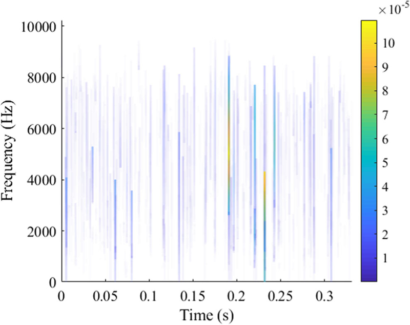
Frequency spectrum of IMF 3
The traditional EMD method is incapable of detecting the fault signal. By examining the Hilbert spectrum in Fig. 17, the EMD method is only sensitive to the high-frequency spectrum in the 3000 to 7000 Hz range, which may be beneficial for high-frequency resonance analysis. However, for rolling element bearing operating at a relative low speed, the lower frequency components contain more direct information indicating the health state of the machinery.
4. Conclusions
In this paper, a nonlinear adaptive dictionary learning algorithm for bearing diagnosis is proposed. The proposed model uses the SE and SES Infogram with added capability to analyze cyclostationary signal as a preprocessing tool to acquire the training data for the dictionary. The filtered signal contains the bearing fault frequency and its harmonics buried in the system noise. A nonlinear map is created between the artificially created kurtosis and the weights of the dictionaries. The UKF is implemented to update the weights of a randomly initialized dictionary based on artificially created kurtosis and the filtered data from the Infogram. The updated dictionary is used for bearing fault diagnosis. The UKF is computationally cheaper and easier to implement rather than using the traditional K-SVD method in obtaining the dictionary. The proposed model also gives the self-adaptation capability for the dictionary and can be used in online monitoring process. The dictionary learning diagnostic model creates a framework for the adaptive monitoring of the bearing degradation process. It is more robust and flexible than a fixed parameter model such as the wavelet denoising and the Kurtogram. An interesting topic to be investigated, as pointed out at the end, is achieving structural adaptation of the dictionary by eliminating the dictionaries with small weight values. By implementing the structural adaptation, computation effort is guaranteed to be reduced. The performance will need to be evaluated in comparison to the nonstructural adaptation model.
Footnotes
Publisher’s note Springer Nature remains neutral with regard to jurisdictional claims in published maps and institutional affiliations.
References
- 1.Ayhan B, Kwan C, and Liang SY Adaptive remaining useful life prediction algorithm for bearings. In 2018 IEEE International Conference on Prognostics and Health Management (ICPHM) 2018. IEEE. [Google Scholar]
- 2.Randall RB, Antoni J (2011) Rolling element bearing diagnostics— a tutorial. Mech Syst Signal Process 25(2):485–520 [Google Scholar]
- 3.Smith WA, Randall RB (2015) Rolling element bearing diagnostics using the Case Western Reserve University data: a benchmark study. Mech Syst Signal Process 64:100–131 [Google Scholar]
- 4.Antoni J, Randall R (2006) The spectral kurtosis: application to the vibratory surveillance and diagnostics of rotating machines. Mech Syst Signal Process 20(2):308–331 [Google Scholar]
- 5.Lu Y, Li Q, Pan Z, Liang SY (2018) Prognosis of bearing degradation using gradient variable forgetting factor RLS combined with time series model. IEEE Access 6:10986–10,995 [Google Scholar]
- 6.Li Y (1999) Dynamic prognostics of rolling element bearing condition Georgia Institute of Technology [Google Scholar]
- 7.Tavner PJ, Penman J (1987) Condition monitoring of electrical machines, vol 1 John Wiley & Sons Incorporated [Google Scholar]
- 8.Qiu H, Lee J, Lin J, Yu G (2006) Wavelet filter-based weak signature detection method and its application on rolling element bearing prognostics. J Sound Vib 289(4–5):1066–1090 [Google Scholar]
- 9.Huang NE, Shen Z, Long SR, Wu MC, Shih HH, Zheng Q, Yen N-C, Tung CC, Liu HH (1998) The empirical mode decomposition and the Hilbert spectrum for nonlinear and non-stationary time series analysis. In Proceedings of the Royal Society of London A: mathematical, physical and engineering sciences The Royal Society; 454:903–995 [Google Scholar]
- 10.Borghesani P, Ricci R, Chatterton S, Pennacchi P (2013) A new procedure for using envelope analysis for rolling element bearing diagnostics in variable operating conditions. Mech Syst Signal Process 38(1):23–35 [Google Scholar]
- 11.Liu R, Yang B, Zio E, Chen X (2018) Artificial intelligence for fault diagnosis of rotating machinery: a review. Mech Syst Signal Process 108:33–47 [Google Scholar]
- 12.Lu Y, Xie R, Liang SY (2018) Detection of weak fault using sparse empirical wavelet transform for cyclic fault. Int J Adv Manuf Technol:1–7 [PMC free article] [PubMed]
- 13.Zhang Y, Randall R (2009) Rolling element bearing fault diagnosis based on the combination of genetic algorithms and fast kurtogram. Mech Syst Signal Process 23(5):1509–1517 [Google Scholar]
- 14.Randall R, Sawalhi N, Coats M (2011) A comparison of methods for separation of deterministic and random signals. International Journal of Condition Monitoring 1(1):11–19 [Google Scholar]
- 15.Fyfe K, Munck E (1997) Analysis of computed order tracking. Mech Syst Signal Process 11(2):187–205 [Google Scholar]
- 16.Bossley K, Mckendrick R, Harris C, Mercer C (1999) Hybrid computed order tracking. Mech Syst Signal Process 13(4):627–641 [Google Scholar]
- 17.Zhao M, Lin J, Wang X, Lei Y, Cao J (2013) A tacho-less order tracking technique for large speed variations. Mech Syst Signal Process 40(1):76–90 [Google Scholar]
- 18.Ahamed N, Pandya Y, Parey A (2014) Spur gear tooth root crack detection using time synchronous averaging under fluctuating speed. Measurement 52:1–11 [Google Scholar]
- 19.Combet F, Gelman L (2007) An automated methodology for performing time synchronous averaging of a gearbox signal without speed sensor. Mech Syst Signal Process 21(6):2590–2606 [Google Scholar]
- 20.Bonnardot F, El Badaoui M, Randall R, Daniere J, Guillet F (2005) Use of the acceleration signal of a gearbox in order to perform angular resampling (with limited speed fluctuation). Mech Syst Signal Process 19(4):766–785 [Google Scholar]
- 21.Elasha F, RuizCarcel C, Mba D, Chandra P (2014) A comparative study of the effectiveness of adaptive filter algorithms, spectral kurtosis and linear prediction in detection of a naturally degraded bearing in a gearbox. J Fail Anal Prev 14(5):623–636 [Google Scholar]
- 22.Akaike H (1969) Fitting autoregressive models for prediction. Ann Inst Stat Math 21(1):243–247 [Google Scholar]
- 23.Box GE, Jenkins GM, Reinsel GC, Ljung GM (2015) Time series analysis: forecasting and control John Wiley & Sons [Google Scholar]
- 24.Randall RB (2011) Vibration-based condition monitoring: industrial, aerospace and automotive applications John Wiley & Sons [Google Scholar]
- 25.Daubechies I (1990) The wavelet transform, time-frequency localization and signal analysis. IEEE Trans Inf Theory 36(5):961–1005 [Google Scholar]
- 26.Sun Z, Chang C (2002) Structural damage assessment based on wavelet packet transform. J Struct Eng 128(10):1354–1361 [Google Scholar]
- 27.Selesnick IW, Baraniuk RG, Kingsbury NC (2005) The dualtree complex wavelet transform. IEEE Signal Process Mag 22(6):123–151 [Google Scholar]
- 28.Wang D, Tsui K-L (2017) Dynamic Bayesian wavelet transform: new methodology for extraction of repetitive transients. Mech Syst Signal Process 88:137–144 [Google Scholar]
- 29.Yan R, Gao RX, Chen X (2014) Wavelets for fault diagnosis of rotary machines: a review with applications. Signal Process 96:1–15 [Google Scholar]
- 30.Antoni J (2007) Fast computation of the kurtogram for the detection of transient faults. Mech Syst Signal Process 21(1):108–124 [Google Scholar]
- 31.Antoni J (2016) The infogram: Entropic evidence of the signature of repetitive transients. Mech Syst Signal Process 74:73–94 [Google Scholar]
- 32.Mairal J, Bach F, Ponce J, Sapiro G (2009) Online dictionary learning for sparse coding. In Proceedings of the 26th annual international conference on machine learning. ACM. [Google Scholar]
- 33.Mairal J, Bach F, Ponce J, Sapiro G (2010) Online learning for matrix factorization and sparse coding. J Mach Learn Res 11(Jan): 19–60 [Google Scholar]
- 34.Zhang Q, Li B (2010) Discriminative K-SVD for dictionary learning in face recognition. In Computer Vision and Pattern Recognition (CVPR), 2010 IEEE Conference on. IEEE. [Google Scholar]
- 35.Aharon M, Elad M, Bruckstein A (2006) K-SVD: an algorithm for designing overcomplete dictionaries for sparse representation. IEEE Trans Signal Process 54(11):4311–4322 [Google Scholar]
- 36.Skretting K, Engan K (2011) Image compression using learned dictionaries by RLS-DLA and compared with K-SVD. In Acoustics, Speech and Signal Processing (ICASSP), 2011 IEEE International Conference on. IEEE. [Google Scholar]
- 37.Rubinstein R, Peleg T, Elad M (2013) Analysis K-SVD: a dictionarylearning algorithm for the analysis sparse model. IEEE Trans Signal Process 61(3):661–677 [Google Scholar]
- 38.Wang L, Lu K, Liu P, Ranjan R, Chen L (2014) IK-SVD: dictionary learning for spatial big data via incremental atom update. Computing in Science & Engineering 16(4):41–52 [Google Scholar]
- 39.Jiang Z, Lin Z, Davis LS (2011) Learning a discriminative dictionary for sparse coding via label consistent K-SVD. In Computer Vision and Pattern Recognition (CVPR), 2011 IEEE Conference on. IEEE. [DOI] [PubMed] [Google Scholar]
- 40.Tropp JA, Gilbert AC (2007) Signal recovery from random measurements via orthogonal matching pursuit. IEEE Trans Inf Theory 53(12):4655–4666 [Google Scholar]
- 41.Donoho DL, Tsaig Y, Drori I, Starck J-L (2012) Sparse solution of underdetermined systems of linear equations by stagewise orthogonal matching pursuit. IEEE Trans Inf Theory 58(2):1094–1121 [Google Scholar]
- 42.Rubinstein R, Zibulevsky M, Elad M (2008) Efficient implementation of the K-SVD algorithm using batch orthogonal matching pursuit. Cs Technion 40(8):1–15 [Google Scholar]
- 43.Gharavi-Alkhansari M and Huang TS A fast orthogonal matching pursuit algorithm. In Acoustics, Speech and Signal Processing, 1998. Proceedings of the 1998 IEEE International Conference on. 1998. IEEE. [Google Scholar]
- 44.Borghesani P, Pennacchi P, Ricci R, Chatterton S (2013) Testing second order cyclostationarity in the squared envelope spectrum of non-white vibration signals. Mech Syst Signal Process 40(1):38–55 [Google Scholar]
- 45.Feng Z, Ma H, Zuo MJ (2017) Spectral negentropy based sidebands and demodulation analysis for planet bearing fault diagnosis. J Sound Vib 410:124–150 [Google Scholar]
- 46.Nocedal J, Wright SJ (2006) Conjugate gradient methods Numerical optimization:101–134 [Google Scholar]
- 47.Golub GH, Reinsch C (1970) Singular value decomposition and least squares solutions. Numer Math 14(5):403–420 [Google Scholar]
- 48.Julier SJ, Uhlmann JK (1997) New extension of the Kalman filter to nonlinear systems. In Signal processing, sensor fusion, and target recognition VI International Society for Optics and Photonics [Google Scholar]
- 49.Wan EA, Van Der Merwe R (2001) The unscented Kalman filter. Kalman filtering and neural networks:221–280
- 50.Julier SJ, Uhlmann JK (2004) Unscented filtering and nonlinear estimation. Proc IEEE 92(3):401–422 [Google Scholar]
- 51.Box GE, Tiao GC (2011) Bayesian inference in statistical analysis, vol 40 John Wiley & Sons<; /References> [Google Scholar]