Allowing for uncertainty due to missing continuous outcome data in pairwise and network meta‐analysis

Abstract

Missing outcome data are commonly encountered in randomized controlled trials and hence may need to be addressed in a meta‐analysis of multiple trials. A common and simple approach to deal with missing data is to restrict analysis to individuals for whom the outcome was obtained (complete case analysis). However, estimated treatment effects from complete case analyses are potentially biased if informative missing data are ignored. We develop methods for estimating meta‐analytic summary treatment effects for continuous outcomes in the presence of missing data for some of the individuals within the trials. We build on a method previously developed for binary outcomes, which quantifies the degree of departure from a missing at random assumption via the informative missingness odds ratio. Our new model quantifies the degree of departure from missing at random using either an informative missingness difference of means or an informative missingness ratio of means, both of which relate the mean value of the missing outcome data to that of the observed data. We propose estimating the treatment effects, adjusted for informative missingness, and their standard errors by a Taylor series approximation and by a Monte Carlo method. We apply the methodology to examples of both pairwise and network meta‐analysis with multi‐arm trials. © 2014 The Authors. Statistics in Medicine Published by John Wiley & Sons Ltd.

1. Introduction

Even in carefully designed and conducted randomized controlled trials (RCTs), patients may be lost to follow up. Exclusion of missing participants from the analysis may, under some circumstances, reduce precision in the estimated treatment effects and produce biased results. In mental health trials, for instance, the dropout rate is generally high and may exceed 50% 1. It has been shown that patients in a placebo arm may be more likely to drop out because of lack of efficacy, and patients in an active treatment arm may be more likely to drop out because of severe adverse events 2. This corresponds to informatively missing (IM) data 3: reasons for dropout are associated with the outcome measured, given all observed data. Bias is especially likely when reasons for dropout are also associated with the treatment assigned. Failure to account for the missing outcome data in the evidence provided from RCTs and their meta‐analysis can lead to biased conclusions.

The intention‐to‐treat principle is widely accepted as the most appropriate way to analyze RCT data, as it avoids biases caused by participants switching interventions or dropping out of the trial. The intention‐to‐treat principle can only be followed fully if there are complete outcome data for all randomized participants. In an RCT, this is possible when appropriate analysis strategies are employed for the missing outcome data 4.

When conducting a meta‐analysis, however, the data available are usually much simpler: for each arm, just the number of randomized individuals, the number with observed outcome, and simple summaries of the observed outcomes. In this setting, it is common practice to ignore the missing data or consider that the missing data have been handled at the study level (e.g., via an imputation approach). In this paper, however, we assume there has been no imputation at the study level. Ignoring missing outcome data in a complete case (CC) analysis is valid in general when data are missing at random (MAR). For this data structure, MAR means that the probability of data being missing does not depend on the outcome within randomized groups, which is equivalent to missing completely at random within randomized groups. Meta‐analysts typically do not have access to the reasons for missing outcome data, and the MAR assumption cannot be explored empirically. Consequently, a sensitivity analysis is the only viable way to evaluate the effect of different scenarios for the missing data mechanism 5. A review of methods currently used for handling missing outcome data in meta‐analysis can be found in 6.

Typical sensitivity analyses include the best‐case and worst‐case scenarios, defining the extremes that could have occurred had all outcomes been observed. These two extremes may be unrealistic in practice. Gamble and Hollis suggested that studies for which there is a big discrepancy between these two extremes should be downweighted 7. A more elegant way to undertake sensitivity analysis is via a pattern‐mixture model that makes hypotheses for the unobserved data given the observed data 8. For the case of missing binary outcomes, White et al. presented a pattern‐mixture model where the degree of departure from the MAR assumption is quantified by the informative missingness odds ratio (IMOR) 9. The IMOR is defined as the ratio of the odds of success in the missing data to the corresponding odds in the observed data. Higgins et al. provide an overview of imputation strategies for binary data, including the IMOR approach and impute risks among missing participants for each group based on available reasons for missingness 10. An advantage of the IMOR model is that it is plausibly unaffected by the amount of missing data, unlike the similar measure based on the risk ratio suggested by Magder 11. Spineli et al. extended the IMOR to a network meta‐analysis (NMA) setting and explored the impact of missing outcome data on inferences about the relative effectiveness of several competing treatments 12. We see two major advantages of the IMOR approach. First, it does not aim to estimate the missing values but, in the spirit of Shafer and Graham 13, aims to make valid inference on the parameters of interest. Second, it accounts for the uncertainty induced by missing outcome data, unlike naïve approaches that consider the imputed values as if they were fully observed 14.

Little work has been carried out to date for quantitative (continuous) missing outcome data in meta‐analysis. Standard approaches include CC analysis and imputation of the observed means for the missing participants 15. This paper proposes a new pattern‐mixture model for meta‐analysis of trials with a single continuous outcome measured at one time point. Our model enables estimation of summary effects while accounting for uncertainty in the outcome of the participants who dropped out. We allow the treatment effect to be measured as a mean difference (MD), as a standardized MD (SMD), or as a ratio of means. Instead of the IMOR, we quantify the degree of departure from MAR by the informative missingness difference of means (IMDoM) or by the informative missingness ratio of means (IMRoM). We address both pairwise and NMA, and we extend the methods to handle multi‐arm trials.

The paper is laid out as follows. In Section 2, we present the pattern‐mixture model, introduce the measures of departure from MAR, and propose two estimation methods. In Section 3, we present the pairwise and NMA models. In Section 4, the proposed methodology is illustrated in two data sets for pairwise and NMA. We conclude with a discussion in Section 5.

2. Methods

2.1. Notation and model definition

We suppose there are m _ij+n _ij participants randomized in arm of study i, with n _ij participants providing outcome data and m _ij participants for whom outcome data are not available. For individual k = 1,…,m _ij+n _ij in arm j, let Y _ijk be the (possibly missing) outcome, and let the indicator variable R _ijk assume value 1 if the outcome has been observed and 0 otherwise. In this section, we assume two‐arm trials, so j = C for control or T for treatment; In Section 3.2, we extend the model to multi‐arm trials.

We write our model as

$$\begin{array}{cc}P\left(R_{\mathrm{ijk}}=1\right)& ={\pi }_{\mathrm{ij}},\\ E\left(Y_{\mathrm{ijk}}|R_{\mathrm{ijk}}=1\right)& ={\chi }_{\mathrm{ij}}^{\mathrm{obs}},\\ E\left(Y_{\mathrm{ijk}}|R_{\mathrm{ijk}}=0\right)& ={\chi }_{\mathrm{ij}}^{\mathrm{miss}}.\end{array}$$

We use Greek letters π,χ to denote parameters and Latin letters p,x for their sample estimates. We can estimate π _ij and ${\chi }_{\mathrm{ij}}^{\mathrm{obs}}$ directly from the data, whereas ${\chi }_{\mathrm{ij}}^{\mathrm{miss}}$ cannot be estimated from the data. The probability that an individual provides outcome data, π _ij, can be estimated by $p_{\mathrm{ij}}=\frac{n_{\mathrm{ij}}}{m_{\mathrm{ij}}+n_{\mathrm{ij}}}$, and ${\chi }_{\mathrm{ij}}^{\mathrm{obs}}$ is estimated by the sample mean $x_{\mathrm{ij}}^{\mathrm{obs}}$ with variance $\raisebox{1ex}{$s_{ij}^2$}\!\left/ \!\raisebox{-1ex}{$n_{ij}$}\right.$, where s _ij is the standard deviation of the outcome among observed participants.

The unconditional expectation of the outcome in each study arm is

$$E\left(Y_{\mathrm{ijk}}\right)\equiv {\chi }_{\mathrm{ij}}^{\mathrm{tot}}={\pi }_{\mathrm{ij}}{\chi }_{\mathrm{ij}}^{\mathrm{obs}}+(1-{\pi }_{\mathrm{ij}}){\chi }_{\mathrm{ij}}^{\mathrm{miss}}.$$ (1)

The unconditional means ${\chi }_{\mathrm{ij}}^{\mathrm{tot}}$ are contrasted to obtain the relative treatment effect in each study, which is defined as the difference

$${\beta }_i\equiv f\left({\chi }_{\mathrm{iT}}^{\mathrm{tot}}\right)-f\left({\chi }_{\mathrm{iC}}^{\mathrm{tot}}\right)$$ (2)

where f is a link function that determines the effect measure. β _i is the MD if f(u) = u; the logarithm of the ratio of means (ln RoM) if f(u)= ln(u) 16; and the SMD if $f\left(u_i\right)=\frac{u_i}{s_i}$, where $s_i=\sqrt{\frac{(n_{\mathrm{iT}}-1)s_{\mathrm{iT}}^2+(n_{\mathrm{iC}}-1)s_{\mathrm{iC}}^2}{n_{\mathrm{iT}}+n_{\mathrm{iC}}-2}}$ is the usual pooled standard deviation.

2.2. Quantifying informative missingness: connecting mean outcome values between observed and missing data

We quantify informative missingness (IM) by making assumptions about the relationship between the outcome means from the observed data and missing data. Specifically, we set

$${\lambda }_{\mathrm{ij}}=g\left({\chi }_{\mathrm{ij}}^{\mathrm{miss}}\right)-g\left({\chi }_{\mathrm{ij}}^{\mathrm{obs}}\right)$$ (3)

so that the mean value in the missing data in study i and arm j is related to the corresponding mean of the observed data by an unknown parameter λ _ij. Equation (1) implies that ${\chi }_{\mathrm{ij}}^{\mathrm{miss}}=g^{-1}\left({\lambda }_{\mathrm{ij}}+g\left({\chi }_{\mathrm{ij}}^{\mathrm{obs}}\right)\right)$. We consider two options for the link function g:

1. If g is the identity function, ${\lambda }_{\mathrm{ij}}={\chi }_{\mathrm{ij}}^{\mathrm{miss}}-{\chi }_{\mathrm{ij}}^{\mathrm{obs}}$ is the IMDoM.

2. If g is the ln function, $\exp \left({\lambda }_{\mathrm{ij}}\right)=\underset{\mathrm{ij}}{\overset{\mathrm{miss}}{\chi }}/{\chi }_{\mathrm{ij}}^{\mathrm{obs}}$ is the IMRoM.

From Equations (1) and (3), it follows that

$${\chi }_{\mathrm{ij}}^{\mathrm{tot}}={\pi }_{\mathrm{ij}}{\chi }_{\mathrm{ij}}^{\mathrm{obs}}+\left(1-{\pi }_{\mathrm{ij}}\right)g^{-1}\left({\lambda }_{\mathrm{ij}}+g\left({\chi }_{\mathrm{ij}}^{\mathrm{obs}}\right)\right).$$ (4)

Under the MAR assumption, λ _ij=0, and consequently, ${\chi }_{\mathrm{ij}}^{\mathrm{obs}}={\chi }_{\mathrm{ij}}^{\mathrm{miss}}={\chi }_{\mathrm{ij}}^{\mathrm{tot}}$. This justifies a CC analysis. Values of λ _ij away from zero reflect IM; for instance, λ _ij<0 means that participants who leave the study have on average a lower outcome than completers. The choice of the treatment effect measure is separate from the choice of the method used to relate ${\chi }_{\mathrm{ij}}^{\mathrm{miss}}$ to ${\chi }_{\mathrm{ij}}^{\mathrm{obs}}$, that is, different choices may be made for the link functions g and f. However, ln RoM is likely to be used in conjunction with IMRoM, and MD and SMD with IMDoM, as they are intuitively related.

We need to make assumptions about the parameter λ _ij, because it is not possible to learn about it from the data. We might choose fixed values, but typically, we are not sure of the value of λ _ij, so we place a distribution on it with mean ${\mu }_{{\lambda }_{\mathrm{ij}}}$ and variance ${\sigma }_{{\lambda }_{\mathrm{ij}}}^2$, written ${\lambda }_{\mathrm{ij}}\sim N\left({\mu }_{{\lambda }_{\mathrm{ij}}},{\sigma }_{{\lambda }_{\mathrm{ij}}}^2\right)$. In all cases, ${\mu }_{{\lambda }_{\mathrm{ij}}}$ describes the most likely MD between the missing and observed outcomes, while ${\sigma }_{{\lambda }_{\mathrm{ij}}}^2$ describes the magnitude of uncertainty around this value. Further assumptions can be considered about the means and variances $\left({\mu }_{{\lambda }_{\mathrm{ij}}}\text{and}{\sigma }_{{\lambda }_{\mathrm{ij}}}^2\right)$ and about the similarity of λ _ij across treatments, in analogy to the models presented in White et al., 17. Specifically, we may consider the following:

• Separate λ _ij for each arm and study, ${\lambda }_{\mathrm{ij}}\sim N\left({\mu }_{{\lambda }_{\mathrm{ij}}},{\sigma }_{{\lambda }_{\mathrm{ij}}}^2\ne 0\right)$, where the λ's are independent both across arms and studies.

• Study‐specific λ:${\lambda }_{\mathrm{ij}}\sim N\left({\mu }_{{\lambda }_i},{\sigma }_{{\lambda }_i}^2\ne 0\right)$, where the λ _i's are independent across studies. The relationship between missing and observed data is different for each study but the same for both arms within a study.

• Correlated across arms. It is assumed that the relation between ${\chi }_{\mathrm{ij}}^{\mathrm{obs}}$ and ${\chi }_{\mathrm{ij}}^{\mathrm{miss}}$ for the two groups (control and treatment) are correlated, $\mathrm{corr}\left({\lambda }_{\mathrm{iC}},{\lambda }_{\mathrm{iT}}\right)={\rho }_{{\lambda }_i}$,

  $$\left(\begin{array}{c}{\lambda }_{\mathrm{iC}}\\ {\lambda }_{\mathrm{iT}}\\ \end{array}\right)\sim N_2\left(\left(\begin{array}{c}{\mu }_{{\lambda }_{\mathrm{iC}}}\\ {\mu }_{{\lambda }_{\mathrm{iT}}}\\ \end{array}\right),\left(\begin{array}{cc}{\sigma }_{{\lambda }_{\mathrm{iC}}}^2& {\rho }_{{\lambda }_i}{\sigma }_{{\lambda }_{\mathrm{iC}}}{\sigma }_{{\lambda }_{\mathrm{iT}}}\\ {\rho }_{{\lambda }_i}{\sigma }_{{\lambda }_{\mathrm{iC}}}{\sigma }_{{\lambda }_{\mathrm{iT}}}& {\sigma }_{{\lambda }_{\mathrm{iT}}}^2\\ \end{array}\right)\right).$$

  Expert opinion can be used to inform the joint distribution of λ _iC and λ _iT. Alternatively, a sensitivity analysis can be adopted to explore how robust the results are to joint distribution for λ _iC and λ _iT.

2.3. Estimation of the relative treatment effect in a single trial

We are interested in estimating the treatment effect β _i and its variance in each study, conditional on the prior distribution of λ _ij and the data $x_{\mathrm{iT}}^{\mathrm{obs}},x_{\mathrm{iC}}^{\mathrm{obs}},s_{\mathrm{iT}},s_{\mathrm{iC}},n_{\mathrm{iT}},n_{\mathrm{iC}},m_{\mathrm{iT}}$, and m _iC. This is therefore a two‐stage approach: in the first stage, we adjust effect sizes and their variances in each study for the IM data, while in the second stage, we pool the adjusted effect sizes. We present two methods for estimating β _i and its uncertainty. We first consider full Bayesian inference and Monte Carlo integration, which we take to be the gold standard. As this approach can be computationally slow, we also present an approximate method based on a Taylor series approximation. Pooling of results across studies is described in Section 3.

2.3.1. Estimation using Monte Carlo integration (parametric bootstrapping)

We use the likelihood function for a study i, l(data _i|θ _i), where ${\mathit{\theta }}_i=\left({\chi }_{\mathrm{iT}}^{\mathrm{obs}},{\pi }_{\mathrm{iT}},{\lambda }_{\mathrm{iT}},{\chi }_{\mathrm{iC}}^{\mathrm{obs}},{\pi }_{\mathrm{iC}},{\lambda }_{\mathrm{iC}}\right)$, and prior information for θ _i, which is expressed as a probability density function h(θ _i) before observing any data. The IM parameter (λ _iT,λ _iC) has the informative prior specified in Section 2.2, whereas $\left({\chi }_{\mathrm{iT}}^{\mathrm{obs}},{\pi }_{\mathrm{iT}},{\chi }_{\mathrm{iC}}^{\mathrm{obs}},{\pi }_{\mathrm{iC}}\right)$ have independent noninformative priors. ${\chi }_{\mathrm{ij}}^{\mathrm{miss}}$ does not appear in θ _i because it is a function of ${\chi }_{\mathrm{ij}}^{\mathrm{obs}}$ and λ _ij. The prior beliefs are updated via the likelihood function to yield the posterior distribution for θ _i via Bayes' theorem $h\left({\mathit{\theta }}_i|{\mathit{\text{data}}}_{\mathit{i}}\right)=\frac{l\left({\mathit{\text{data}}}_{\mathit{i}}|{\mathit{\theta }}_i\right)h\left({\mathit{\theta }}_i\right)}{\underset{R_{{\mathit{\theta }}_i}}{\int }l\left({\mathit{\text{data}}}_{\mathit{i}}|{\mathit{\theta }}_i\right)h\left({\mathit{\theta }}_i\right)d{\mathit{\theta }}_i}$, where the denominator is a normalizing constant and $R_{{\theta }_i}$ is the set of possible values for θ _i. The posterior distribution expresses the probability distribution of θ _i after observing the data. Missingness parameters λ _i cannot be informed by the data, and their prior distribution is identical to the posterior. This stresses the importance of the prior distribution to be assigned.

We are interested in estimating β _i, which can be written as β(θ _i) using (2) and (4). Specifically, we compute the expected value of β(θ _i) over the posterior distribution of θ _i, that is, $E\left(\beta \left({\mathit{\theta }}_i\right)|{\mathit{\text{data}}}_{\mathit{i}}\right)=\underset{R_{{\mathit{\theta }}_i}}{\int }\beta \left({\mathit{\theta }}_i\right)h\left({\mathit{\theta }}_i|{\mathit{\text{data}}}_{\mathit{i}}\right)d{\mathit{\theta }}_i$, and the corresponding variance. The integrals are calculated using Monte Carlo integration using a large number of samples, selected randomly from h(θ _i|data _i). We repeat the following procedure, indexed with b, a large number of times B for each i,j:

1. Draw ${\left({\chi }_{\mathrm{ij}}^{\mathrm{obs}}\right)}^b$ from ${\left({\chi }_{\mathrm{ij}}^{\mathrm{obs}}\right)}^b\sim N\left(x_{\mathrm{ij}}^{\mathrm{obs}},\frac{s_{\mathrm{ij}}^2}{n_{\mathrm{ij}}}\right)$.

2. Draw ${\lambda }_{\mathrm{ij}}^b$ from ${\lambda }_{\mathrm{ij}}^b\sim N\left({\mu }_{{\lambda }_{\mathrm{ij}}},{\sigma }_{{\lambda }_{\mathrm{ij}}}^2\right)$.

3. Set ${\left({\chi }_{\mathrm{ij}}^{\mathrm{miss}}\right)}^b={\lambda }_{\mathrm{ij}}^b+{\left({\chi }_{\mathrm{ij}}^{\mathrm{obs}}\right)}^b$ for IMDoM or ${\left({\chi }_{\mathrm{ij}}^{\mathrm{miss}}\right)}^b=e^{{\lambda }_{\mathrm{ij}}^b}{\left({\chi }_{\mathrm{ij}}^{\mathrm{obs}}\right)}^b$ for IMRoM.

4. Draw the nonmissing rate ${\pi }_{\mathrm{ij}}^b$ from ${\pi }_{\mathrm{ij}}^b\sim N\left(p_{\mathrm{ij}},\frac{p_{\mathrm{ij}}(1-p_{\mathrm{ij}})}{n_{\mathrm{ij}}+m_{\mathrm{ij}}}\right)$.

5. Compute ${\left({\chi }_{\mathrm{ij}}^{\mathrm{tot}}\right)}^b={\pi }_{\mathrm{ij}}^b{\left({\chi }_{\mathrm{ij}}^{\mathrm{obs}}\right)}^b+\left(1-{\pi }_{\mathrm{ij}}^b\right){\left({\chi }_{\mathrm{ij}}^{\mathrm{miss}}\right)}^b$.

Steps 1 and 4 use large sample approximations to the t‐distribution and the beta distribution, respectively.

Finally, for each i, we compute the effect sizes ${\left({\beta }_i\right)}^b=f\left({\left({\chi }_{\mathrm{iT}}^{\mathrm{tot}}\right)}^b\right)-f\left({\left({\chi }_{\mathrm{iC}}^{\mathrm{tot}}\right)}^b\right)$. The mean and variance of (β _i)^b across all Monte Carlo samples b = 1,…,B estimate E(β _i|data _i) and V _i=var(β _i|data _i), respectively.

When λ _iT and λ _iC are correlated, we modify step 2 of the aforementioned procedure by sampling λ _i=(λ _iC,λ _iT)^′ from a joint bivariate normal distribution.

2.3.2. Estimation using a Taylor approximation

2.3.2.1. Estimating the mean effect size

We first estimate $E\left({\chi }_{\mathrm{ij}}^{\mathrm{tot}}|{\mathit{\text{data}}}_{\mathit{i}}\right)$. For IMDoM, Equation (4) simplifies to $E\left({\chi }_{\mathrm{ij}}^{\mathrm{tot}}|{\lambda }_{\mathrm{ij}},{\mathit{\text{data}}}_{\mathit{i}}\right)=\left(1-p_{\mathrm{ij}}\right){\lambda }_{\mathrm{ij}}+x_{\mathrm{ij}}^{\mathrm{obs}}$, which implies $E\left({\chi }_{\mathrm{ij}}^{\mathrm{tot}}|{\mathit{\text{data}}}_{\mathit{i}}\right)=\left(1-p_{\mathrm{ij}}\right){\mu }_{{\lambda }_{\mathrm{ij}}}+x_{\mathrm{ij}}^{\mathrm{obs}}$. For IMRoM, Equation (4) simplifies to $E\left({\chi }_{\mathrm{ij}}^{\mathrm{tot}}|{\lambda }_{\mathrm{ij}},{\mathit{\text{data}}}_{\mathit{i}}\right)=\left(p_{\mathrm{ij}}+\left(1-p_{\mathrm{ij}}\right)e^{{\lambda }_{\mathrm{ij}}}\right)x_{\mathrm{ij}}^{\mathrm{obs}}$, which implies $E\left({\chi }_{\mathrm{ij}}^{\mathrm{tot}}|{\mathit{\text{data}}}_{\mathit{i}}\right)=\left(p_{\mathrm{ij}}+\left(1-p_{\mathrm{ij}}\right)E\left(e^{{\lambda }_{\mathrm{ij}}}\right)\right)x_{\mathrm{ij}}^{\mathrm{obs}}$. Both equations reduce to $E\left({\chi }_{\mathrm{ij}}^{\mathrm{tot}}|{\mathit{\text{data}}}_{\mathit{i}}\right)=x_{\mathrm{ij}}^{\mathrm{obs}}$ when λ _ij=0.

We now have the expected value of β _i conditional on the data:

$$\begin{array}{cc}E\left({\beta }_i|{\mathit{\text{data}}}_{\mathit{i}}\right)& =E\left(f\left({\chi }_{\mathrm{iT}}^{\mathrm{tot}}|{\mathit{\text{data}}}_{\mathit{i}}\right)\right)-E\left(f\left({\chi }_{\mathrm{iC}}^{\mathrm{tot}}|{\mathit{\text{data}}}_{\mathit{i}}\right)\right)\\ \approx f\left(E\left({\chi }_{\mathrm{iT}}^{\mathrm{tot}}|{\mathit{\text{data}}}_{\mathit{i}}\right)\right)-f\left(E\left({\chi }_{\mathrm{iC}}^{\mathrm{tot}}|{\mathit{\text{data}}}_{\mathit{i}}\right)\right).\end{array}$$

2.3.2.2. Estimating the variance of the mean effect size

The variance of β _i conditional on the data can be approximated from the observed data using another Taylor series approximation of Equation (2).

$$\begin{array}{cc}{V}_i& =\mathrm{var}\left({\beta }_i|{\mathit{\text{data}}}_{\mathit{i}}\right)\approx \mathrm{var}\left({\chi }_{\mathrm{iT}}^{\mathrm{tot}}|{\mathit{\text{data}}}_{\mathit{i}}\right)f^{\prime }{\left({\chi }_{\mathrm{iT}}^{\mathrm{tot}}\right)}^2\\ +\mathrm{var}\left({\chi }_{\mathrm{iC}}^{\mathrm{tot}}|{\mathit{\text{data}}}_{\mathit{i}}\right)f^{\prime }{\left({\chi }_{\mathrm{iC}}^{\mathrm{tot}}\right)}^2-2\text{cov}\left({\chi }_{\mathrm{iT}}^{\mathrm{tot}},{\chi }_{\mathrm{iC}}^{\mathrm{tot}}|{\mathit{\text{data}}}_{\mathit{i}}\right)f^{\prime }\left({\chi }_{\mathrm{iT}}^{\mathrm{tot}}\right)f^{\prime }\left({\chi }_{\mathrm{iC}}^{\mathrm{tot}}\right).\end{array}$$ (5)

The covariance term in Equation (5) is only needed if λ _iC and λ _iT are correlated.

We show how to evaluate the variances $\mathrm{var}\left({\chi }_{\mathrm{iT}}^{\mathrm{tot}}|{\mathit{\text{data}}}_{\mathit{i}}\right)$ and covariance $\text{cov}\left({\chi }_{\mathrm{iT}}^{\mathrm{tot}},{\chi }_{\mathrm{iC}}^{\mathrm{tot}}|{\mathit{\text{data}}}_{\mathit{i}}\right)$ in the succeeding text. The derivative of the link function f ^′(u) is 1 for MD, 1/^u for ln RoM, and $\frac{1}{s_i}$ for SMD.

To obtain $\mathrm{var}\left({\chi }_{\mathrm{ij}}^{\mathrm{tot}}|{\mathit{\text{data}}}_{\mathit{i}}\right)$, we first use a Taylor series approximation of $\mathrm{var}\left({\chi }_{\mathrm{ij}}^{\mathrm{tot}}|{\lambda }_{\mathrm{ij}},{\mathit{\text{data}}}_{\mathit{i}}\right)$ about sample estimators $x_{\mathrm{ij}}^{\mathrm{obs}}$ and p _ij:

$$\mathrm{var}\left({\chi }_{\mathrm{ij}}^{\mathrm{tot}}|{\lambda }_{\mathrm{ij}},{\mathit{\text{data}}}_{\mathit{i}}\right)\approx \mathrm{var}\left({\pi }_{\mathrm{ij}}|{\lambda }_{\mathrm{ij}},{\mathit{\text{data}}}_{\mathit{i}}\right){\left(\frac{d{\chi }_{\mathrm{ij}}^{\mathrm{tot}}}{d{\pi }_{\mathrm{ij}}}\right)}^2+\mathrm{var}\left({\chi }_{\mathrm{ij}}^{\mathrm{obs}}|{\lambda }_{\mathrm{ij}},{\mathit{\text{data}}}_{\mathit{i}}\right){\left(\frac{d{\chi }_{\mathrm{ij}}^{\mathrm{tot}}}{d{\chi }_{\mathrm{ij}}^{\mathrm{obs}}}\right)}^2$$

In the preceding text, we estimate the variances as

$$\mathrm{var}\left({\pi }_{\mathrm{ij}}|{\lambda }_{\mathrm{ij}},{\mathit{\text{data}}}_{\mathit{i}}\right)=\frac{p_{\mathrm{ij}}\left(1-p_{\mathrm{ij}}\right)}{n_{\mathrm{ij}}+m_{\mathrm{ij}}},\mathrm{var}\left({\chi }_{\mathrm{ij}}^{\mathrm{obs}}|{\lambda }_{\mathrm{ij}},{\mathit{\text{data}}}_{\mathit{i}}\right)=\frac{s_{\mathrm{ij}}^2}{n_{\mathrm{ij}}};$$

and the derivatives as

$$\frac{d{\chi }_{\mathrm{ij}}^{\mathrm{tot}}}{d{\pi }_{\mathrm{ij}}}=-{\lambda }_{\mathrm{ij}},\frac{d{\chi }_{\mathrm{ij}}^{\mathrm{tot}}}{d{\chi }_{\mathrm{ij}}^{\mathrm{obs}}}=1$$

when the link function g is the identity and

$$\frac{d{\chi }_{\mathrm{ij}}^{\mathrm{tot}}}{d{\pi }_{\mathrm{ij}}}=\left(1-e^{{\lambda }_{\mathrm{ij}}}\right)x_{\mathrm{ij}}^{\mathrm{obs}},\frac{d{\chi }_{\mathrm{ij}}^{\mathrm{tot}}}{d{\chi }_{\mathrm{ij}}^{\mathrm{obs}}}=\left(1-{\pi }_{\mathrm{ij}}\right)e^{{\lambda }_{\mathrm{ij}}}+{\pi }_{\mathrm{ij}}.$$

when g is the log function. To allow for the uncertainty in λ _i, we use $\mathrm{var}\left({\chi }_{\mathrm{ij}}^{\mathrm{tot}}\left|\mathit{\text{data}}\right.\right)=E\left[\mathrm{var}\left({\chi }_{\mathrm{ij}}^{\mathrm{tot}}\left|{\lambda }_{\mathrm{ij}},\mathit{\text{data}}\right.\right)\right]+\mathrm{var}\left[E\left({\chi }_{\mathrm{ij}}^{\mathrm{tot}}\left|{\lambda }_{\mathrm{ij}},\mathit{\text{data}}\right.\right)\right]$. The first term is approximated by $\mathrm{var}\left({\chi }_{\mathrm{ij}}^{\mathrm{tot}}\left|{\lambda }_{\mathrm{ij}}={\mu }_{{\lambda }_{\mathrm{ij}}},\mathit{\text{data}}\right.\right)$. The second term is ${(1-p_{\mathrm{ij}})}^2{\sigma }_{{\lambda }_{\mathrm{ij}}}^2$ for IMDoM and ${(1-p_{\mathrm{ij}})}^2{x}_{\mathrm{ij}}^2\mathrm{var}\left(e^{{\lambda }_{\mathrm{ij}}}\right)$ for IMRoM.

To obtain $\text{cov}\left({\chi }_{\mathrm{iT}}^{\mathrm{tot}},{\chi }_{\mathrm{iC}}^{\mathrm{tot}}|{\mathit{\text{data}}}_{\mathit{i}}\right)$, the Taylor series approximation gives a term, which is proportional to the correlation ${\rho }_{{\lambda }_i}$: $(1-p_{\mathrm{ij}})(1-p_{\mathrm{ik}}){\rho }_{{\lambda }_i}{\sigma }_{{\lambda }_{\mathrm{ij}}}{\sigma }_{{\lambda }_{\mathrm{ik}}}$ for IMDoM and $(1-p_{\mathrm{ij}})(1-p_{\mathrm{ik}})x_{\mathrm{ij}}{x}_{\mathrm{ik}}\text{cov}\left(e^{{\lambda }_{\mathrm{ij}}},e^{{\lambda }_{\mathrm{ik}}}\right)$ for IMRoM. This completes the calculation of Equation (5).

For example, the variance of the MD using IMDoM is

$$V_i\approx \sum _{j=C,T}\left[\frac{p_{\mathrm{ij}}\left(1-p_{\mathrm{ij}}\right)}{n_{\mathrm{ij}}+m_{\mathrm{ij}}}\left({\mu }_{{\lambda }_{\mathrm{ij}}}^2+{\sigma }_{{\lambda }_{\mathrm{ij}}}^2\right)+\frac{s_{\mathrm{ij}}^2}{n_{\mathrm{ij}}}+{\sigma }_{{\lambda }_{\mathrm{ij}}}^2{\left(1-p_{\mathrm{ij}}\right)}^2\right]-2{\rho }_{{\lambda }_i}{\sigma }_{{\lambda }_{\mathrm{iC}}}{\sigma }_{{\lambda }_{\mathrm{iT}}}\left(1-p_{\mathrm{iT}}\right)\left(1-p_{\mathrm{iC}}\right)$$

Expressions for the mean, variance, and covariance are summarized in Table 1.

Table 1.

Estimated means $E\left({\chi }_{\mathrm{ij}}^{\mathrm{tot}}\right|{\lambda }_{\mathrm{ij}},{\mathit{data}}_{\mathit{i}})$ and variances var$\left(E\right({\chi }_{\mathrm{ij}}^{\mathrm{tot}}|{\lambda }_{\mathrm{ij}},{\mathit{data}}_{\mathit{i}}))$ for arm j in study i under both informative missingness difference of means and informative missingness ratio of means.

Parameter	Estimated mean in arm j	Variance in arm j	Covariance between arms j and k
π ij Probability to complete the study	p ij	$\frac{p_{\mathrm{ij}}(1-p_{\mathrm{ij}})}{n_{\mathrm{ij}}+m_{\mathrm{ij}}}$	0
${\chi }_{\mathrm{ij}}^{\mathrm{obs}}$ Mean outcome in participants who completed the study	$x_{\mathrm{ij}}^{\mathrm{obs}}$	$\frac{s_{\mathrm{ij}}^2}{n_{\mathrm{ij}}}$	0
${\chi }_{\mathrm{ij}}^{\mathrm{tot}}\text{(IMDoM)}$ Mean outcome in participants who completed the study assuming a difference in the outcome between missing and observed participants	$\left(1-p_{\mathrm{ij}}{\mu }_{{\lambda }_{\mathrm{ij}}}+x_{\mathrm{ij}}^{\mathrm{obs}}\right)$	$\begin{array}{c}\frac{p_{\mathrm{ij}}(1-p_{\mathrm{ij}})}{n_{\mathrm{ij}}+m_{\mathrm{ij}}}\left({\mu }_{{\lambda }_{\mathrm{ij}}}+{\sigma }_{{\lambda }_{\mathrm{ij}}}^2\right)\\ +\frac{s_{\mathrm{ij}}^2}{n_{\mathrm{ij}}}+{\sigma }_{{\lambda }_{\mathrm{ij}}}{s}_{\mathrm{ij}}^2{(1-p_{\mathrm{ij}})}^2\end{array}$	${\rho }_{{\lambda }_i}{\sigma }_{{\lambda }_{\mathrm{ij}}}{\sigma }_{{\lambda }_{\mathrm{ik}}}(1-p_{\mathrm{ij}})(1-p_{\mathrm{ik}})$
${\chi }_{\mathrm{ij}}^{\mathrm{tot}}\text{(IMRoM)}$ Mean outcome in participants who completed the study assuming a difference in logarithm of the outcome between missing and observed participants	$\left(p_{\mathrm{ij}}+(1-p_{\mathrm{ij}})E\left(e^{{\lambda }_{\mathrm{ij}}}\right)\right)x_{\mathrm{ij}}^{\mathrm{obs}}$	$\begin{array}{c}\frac{p_{\mathrm{ij}}(1-p_{\mathrm{ij}})}{n_{\mathrm{ij}}+m_{\mathrm{ij}}}E\left[{\left(1-e^{{\lambda }_{\mathrm{ij}}}\right)}^2\right]{\left(x_{\mathrm{ij}}^{\mathrm{obs}}\right)}^2\\ +\frac{s_{\mathrm{ij}}^2}{n_{\mathrm{ij}}}E\left[{\left((1-p_{\mathrm{ij}})e^{{\lambda }_{\mathrm{ij}}}+p_{\mathrm{ij}}\right)}^2\right]\\ +\mathrm{var}\left(e^{{\lambda }_{\mathrm{ij}}}\right){\left((1-p_{\mathrm{ij}})x_{\mathrm{ij}}^{\mathrm{obs}}\right)}^2\end{array}$	$\text{cov}(e^{{\lambda }_{ij}},e^{{\lambda }_{ij}})\times (1-p_{ij})(1-p_{ik})x_{ij}{x}_{ik}$
	$\begin{array}{c}\text{where}E\left(e^{{\lambda }_{\mathrm{ij}}}\right)=e^{{\mu }_{{\lambda }_{\mathrm{ij}}}+\frac{1}{2}{\sigma }_{{\lambda }_{\mathrm{ij}}}^2}\text{andvar}\left(e^{{\lambda }_{\mathrm{ij}}}\right)=e^{2{\mu }_{{\lambda }_{\mathrm{ij}}}+{\sigma }_{{\lambda }_{\mathrm{ij}}}^2\left(e^{{\sigma }_{{\lambda }_{\mathrm{ij}}}^2}-1\right)}\\ \mathit{\text{corr}}\left(e^{{\lambda }_{\mathrm{iC}}},e^{{\lambda }_{\mathrm{iT}}}\right)=e^{{\mu }_{{\lambda }_{\mathrm{iC}}}+{\mu }_{\mathrm{\lambda T}}+0.5\left({\sigma }_{{\lambda }_{\mathrm{iC}}}^2+{\sigma }_{{\lambda }_{\mathrm{iT}}}^2\right)}\left(e^{{\rho }_{\lambda }{\sigma }_{{\lambda }_{\mathrm{iC}}}{\sigma }_{{\lambda }_{\mathrm{iT}}}}-1\right)\end{array}$

IMDoM, informative missingness difference of means; IMRoM, informative missingness ratio of means.

In the Appendix, we provide the variances for all three effect sizes under both IMDoM and IMRoM. In all expressions in the appendix, setting ${\mu }_{{\lambda }_{\mathrm{ij}}}={\sigma }_{{\lambda }_{\mathrm{ij}}}=0$ gives β _i=x _iT−x _iC and $V_i=\sum _{j=C,T}\frac{s_{\mathrm{ij}}^2}{n_{\mathrm{ij}}}$, which correspond to a CC analysis.

3. Pairwise meta‐analysis and network meta‐analysis models

We showed in Section 2.3 how to estimate ${\widehat{\beta }}_i=E\left({\beta }_i|{\mathit{\text{data}}}_{\mathit{i}}\right)$ and ${\widehat{V}}_i$ for each study accounting for missing data. We now describe how to pool the adjusted estimates ${\widehat{\beta }}_i$.

3.1. Pairwise meta‐analysis

In a random‐effects meta‐analysis model, for a study i, the estimated from Equation (2) effect size ${\widehat{\beta }}_i$ is modelled as

$${\widehat{\beta }}_i=\mu +{\delta }_i+{\epsilon }_i,$$

where μ is the true effect of active treatment relative to the control treatment, δ _i is a random effect with δ _i∼N(0,τ ²), where the between‐study variance (heterogeneity) τ ² expresses how effectiveness varies across studies, and ε _i is a sampling error term with ε _i∼N(0,V _i). In matrix notation, the model can be expressed as

$$\widehat{\beta }=\mathbf{X}\mathit{\mu }+\delta +\epsilon$$ (6)

where $\widehat{\beta }$ is aⁿ‐vector including the adjusted effect sizes for each study, ε is a n‐vector of normally distributed sampling errors with $\mathit{\epsilon }\sim N_n\left(\mathbf{0},\widehat{V}\right)$ and known diagonal covariance matrix $\widehat{V}=\mathrm{diag}\left({\widehat{V}}_1,\dots ,{\widehat{V}}_n\right),\delta$ is a n‐vector of normally distributed random effects, δ ∼ N _n(0,Δ) with a diagonal covariance matrix Δ = τ ² I _n, and X is a column vector of ones. The summary estimates are computed using weighted least squares giving $\widehat{\mu }={\left(X^{\prime }\widehat{W}X\right)}^{-1}{X}^{\prime }\widehat{W}\widehat{\beta }$ and $\mathrm{var}\left(\widehat{\mu }\right)={\left(X^{\prime }\widehat{W}X\right)}^{-1}$ with weights given by $\widehat{W}=\mathrm{diag}\left({\widehat{W}}_1,\dots ,{\widehat{W}}_n\right)$ and ${\widehat{W}}_i={({\mathbf{V}}_i+\widehat{\mathrm{\Delta }})}^{-1}$. Accounting for missing outcome data typically may change ${\widehat{\beta }}_i$ and increases V _i unless ${\mu }_{{\lambda }_{\mathrm{ij}}}={\sigma }_{{\lambda }_{\mathrm{ij}}}=0$. Hence, the weight matrix changes and so does $\widehat{\mu }$ and $\mathrm{var}\left(\widehat{\mu }\right)$. In practice, the studies with large missing rates have their variances increased and their weight in a meta‐analysis decreased.

3.2. Network meta‐analysis

Network meta‐analysis synthesizes both direct and indirect evidence and provides a ranking of available treatments 18. A key assumption in NMA is that of transitivity implying that the distribution of effect modifiers is similar across treatment comparisons. Statistically, this is explored via the consistency equations, which state that direct and indirect evidence is in agreement. Suppose, for example, we have three treatments A, B, and C and three studies AB, AC, and BC (where AB refers to direct comparison A versus B). Then consistency states that the direct estimate for the relative effectiveness between B and C (μ _BC) equals the indirect estimate obtained by comparing B and C to a common comparator A (μ _AC−μ _AB). In a NMA with T treatments, we select a reference treatment and estimate T − 1 basic contrasts that represent the effectiveness of each of the remaining treatments relative to the reference one. The remaining parameters are estimated through the consistency equations. In the aforementioned example, if A is the reference treatment, then μ _AB and μ _AC are the basic contrasts and μ _BC is estimated as μ _BC=μ _AC−μ _AB. The NMA model is expressed through Equation (6), but μ is now a T − 1 vector of the basic contrasts, and the design matrix X indicates the treatment comparisons in each study under the consistency assumption 19.

Multi‐arm trials complicate this procedure. In a three‐arm trial, we estimate two effect sizes, for example, β _i=(β _iAB,β _iAC)^′, where ${\beta }_{\mathrm{iAj}}=f\left({\chi }_{\mathrm{ij}}^{\mathrm{tot}}\right)-f\left({\chi }_{\mathrm{iA}}^{\mathrm{tot}}\right)$ with j = B,C. We need to estimate the covariance of the two components β _iAB and β _iAC, which arises because they include the same control A and because they may have correlated λ _ij. This is handled in the Monte Carlo scheme of Section 2.3.1 by simulating ${\chi }_{\mathrm{iB}}^{\mathrm{tot}}$ and ${\chi }_{\mathrm{iC}}^{\mathrm{tot}}$ from a bivariate normal in step 1. For the Taylor series approximation of Section 2.3.2, the covariance is

$$\begin{array}{cc}\text{cov}\left({\beta }_{\mathrm{iAB}},{\beta }_{\mathrm{iAC}}|{\mathit{\text{data}}}_{\mathit{i}}\right)& \approx \text{cov}\left({\chi }_{\mathrm{iB}}^{\mathrm{tot}},{\chi }_{\mathrm{iC}}^{\mathrm{tot}}|{\mathit{\text{data}}}_{\mathit{i}}\right)f^{\prime }\left({\chi }_{\mathrm{iB}}^{\mathrm{tot}}\right)f^{\prime }\left({\chi }_{\mathrm{iB}}^{\mathrm{tot}}\right)-\text{cov}\left({\chi }_{\mathrm{iA}}^{\mathrm{tot}},{\chi }_{\mathrm{iB}}^{\mathrm{tot}}|{\mathit{\text{data}}}_{\mathit{i}}\right)f^{\prime }\left({\chi }_{\mathrm{iA}}^{\mathrm{tot}}\right)f^{\prime }\left({\chi }_{\mathrm{iB}}^{\mathrm{tot}}\right)\\ -\text{cov}\left({\chi }_{\mathrm{iA}}^{\mathrm{tot}},{\chi }_{\mathrm{iC}}^{\mathrm{tot}}|{\mathit{\text{data}}}_{\mathit{i}}\right)f^{\prime }\left({\chi }_{\mathrm{iA}}^{\mathrm{tot}}\right)f^{\prime }\left({\chi }_{\mathrm{iC}}^{\mathrm{tot}}\right)+\mathrm{var}\left({\chi }_{\mathrm{iA}}^{\mathrm{tot}}|{\mathit{\text{data}}}_{\mathit{i}}\right)f^{\prime }{\left({\chi }_{\mathrm{iA}}^{\mathrm{tot}}\right)}^2\end{array}$$

and all these terms have been evaluated in Section 2.3.2.

We have uploaded MATLAB 20 code for the suggested methodology at www.mtm.uoi.gr, and we will soon upload a Stata 21 routine.

4. Applications to pairwise meta‐analysis and network meta‐analysis

The suggested methods are illustrated via two examples. The first example synthesizes eight studies comparing the effectiveness of mirtazapine (T) and placebo (C) in patients with major depression 22. The outcome is the change in depression symptoms measured on a standardized rating scale, the HAMD21 scale. For each study arm, we have the mean change, the standard deviation, the number of patients randomized to this arm, and the number of completers (Table 2). We analyze the data using all effect sizes presented in Section 2.1 (MD, SMD, and ln RoM).

Table 2.

Mirtazapine meta‐analysis: mean change in HAMD21 scores, standard deviations, and numbers of completers and noncompleters for the mirtazapine and placebo arms.

Study	Placebo				Mirtazapine
	x obs	s obs	n	m	x obs	s obs	n	m
Claghorn 1995	−11.4	10.2	19	26	−14.5	8.8	26	19
MIR 003‐003	−11.5	8.3	24	21	−14	7.3	27	18
MIR 003‐008	−11.4	8	17	13	−13.2	8	12	18
MIR 003‐020	−6.2	6.5	24	19	−13	9	23	21
MIR 003‐021	−17.4	5.3	21	29	−13.8	5.9	22	28
MIR 003‐024	−11.1	9.9	27	23	−15.7	6.7	30	20
MIR 84023a	−11.9	8.6	33	24	−14.2	7.6	35	25
MIR 84023b	−11.8	8.3	48	18	−14.7	8.4	51	13

We demonstrate how we add uncertainty because of IM data in the fifth study in Table 2 (MIR 003‐021). For the placebo arm, the variance of ${\chi }_{5C}^{\mathrm{tot}}$ is $\frac{{\left(s_{5C}^{\mathrm{obs}}\right)}^2}{n_{5C}}=1.34$ if we assume MAR. Suppose that we use effect measure MD and an IMDoM scenario where λ follows $N\left({\mu }_{{\lambda }_{5C}}=0,{\sigma }_{{\lambda }_{5C}}^2=4\right)$. Then, the variance of ${\chi }_{{}_{5C}}^{\mathrm{tot}}$ using the Taylor series approximation is $\frac{p_{5C}\left(1-p_{5C}\right)}{n_{5C}+m_{5C}}\left({\mu }_{{\lambda }_{5C}}^2+{\sigma }_{{\lambda }_{5C}}^2\right)+\frac{s_{5C}^2}{n_{5C}}+{\sigma }_{{\lambda }_{5C}}^2{\left(1-p_{5C}\right)}^2=3.68$. After a similar calculation for the treatment arm, we estimate the treatment effects. If we assume MAR, we obtain ${\widehat{\beta }}_5=3.60$ with ${\widehat{V}}_5=2.92$, whereas if we assume ${\lambda }_{\mathrm{ij}}\sim N\left({\mu }_{{\lambda }_{\mathrm{ij}}}=0,{\sigma }_{{\lambda }_{{}_{\mathrm{ij}}}}^2=4\right)$ independently in the two arms, we obtain ${\widehat{\beta }}_5=3.60$ with ${\widehat{V}}_5=5.56$.

The second example is used to illustrate the application of the method to a group of nine antidepressants compared in 12 studies within the context of an NMA 22. The outcome is change score in depression measured on a standardized rating scale. Data are shown in Table 3, and Figure 1 presents the network plot 23. As studies use two different scales to measure depression, we consider only SMD and ln RoM. These studies were chosen from a large network of antidepressant studies 22, they are not representative of treatment effectiveness and are used for illustrative purposes here. We restricted analysis to this subset of the evidence base because observed mean values in each arm before conducting any imputation strategy (i.e., last observation carried forward) are available only for these 12 studies.

Table 3.

Antidepressants network: study name, treatments compared, and observed mean change in depression score, standard deviations, number of completers, and noncompleters for each arm.

Study	Comparison	Treatment A				Treatment B
	Treatment A versus treatment B	x obs	s obs	n	m	x obs	s obs	n	m
Kato 2006	Fluxovamine versus paroxetine	9	8.65	41	8	4.6	8.65	39	13
Rossini 2002	Fluxovamine versus sertaline	7.56	12.31	39	1	11.27	11.33	45	3
Annseau 1994	Milnacipran versus fluoxetine	17.2	11.1	74	23	14.2	11.1	75	18
Yang 2003	Milnacipran versus sertaline	13.5	2.1	12	15	13.8	1.8	15	11
Eker 2005	Reboxetine versus sertaline	6.55	5.23	20	5	7.76	2.89	21	3
Chen 2001	Sertaline versus venlafaxine	7	5	45	0	6	5	43	1
Shelton 2006	Sertaline versus venlafaxine	9.6	6.2	63	19	8.4	5.4	67	11
Ekselius 1997	Citalopram versus sertaline	10.4	9.12	37	163	11	9.12	55	145
Khanzode 2003	Citalopram versus fluoxetine	15.8	3.3	30	3	18.7	5.1	32	2
Diaz/Martinez 1998	Fluoxetine versus venlafaxine	8.2	7.52	55	20	8.7	7.52	55	15
Amini 2005	Mirtazapine versus fluoxetine	7.4	7.52	16	2	10.4	7.52	15	3
Silverston 1999	Fluoxetine versus venlafaxine	12	8.65	89	32	11.3	8.65	91	37

Figure 1.

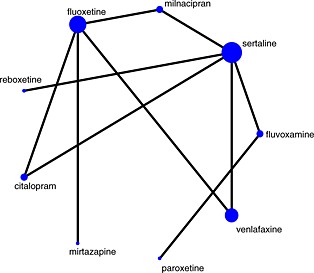
Network plot for comparison of antidepressants. Nodes are weighted according to the number of studies including the respective interventions. Edges are weighted according to the inverse variance of the direct treatment effect estimates for the respective comparisons.

Empirical analysis and simulation findings have shown that ln RoM is a reasonable alternative to SMD for pooling continuous outcomes in meta‐analysis and it does not involve the estimation of the pooled standard deviation, a quantity not well understood by clinicians 16. Like SMD, ln RoM is a unit‐less measure that can be used irrespective of the units of the trial outcome measures, and it requires the means in both arms in all trials included in the meta‐analysis to have the same sign, which is the case in our examples.

4.1. Comparison of Monte Carlo and Taylor estimation methods in a single study

In Section 2.3, we presented two methods for estimating E(β _i|data _i) and V _i=var(β _i|data _i), a Monte Carlo method and a Taylor series approximation. Here, we explore how the posterior mean values and standard error for β _i vary as uncertainty $\left({\sigma }_{{\lambda }_{\mathrm{ij}}}\right)$ in the IM parameters increases for each study under both methods, considering all three different effect sizes (MD, SMD, and ln RoM). For brevity, we present results only for the fifth study in the mirtazapine example (MIR 003‐21 in Table 2), which has a high proportion of missing data: 58% in the placebo group and 56% in the mirtazapine group. We assume a bivariate normal distribution for λ _i=(λ _iC,λ _iT)^′ with mean zero, equal standard deviations in both groups ${\sigma }_{{\lambda }_{\mathrm{iC}}}={\sigma }_{{\lambda }_{\mathrm{iT}}}={\sigma }_{\lambda }$ ranging from 0 to 5 for IMDoM and from 0 to 0.5 for IMRoM, and correlation 0.5. We evaluate the posterior mean and standard error of β ₅ when the effect size is MD, SMD, and ln RoM using (i) Monte Carlo with 10,000 samples and (ii) the Taylor series approximation.

The two methods are compared in Figures 2 and 3 for IMDoM and IMRoM, respectively. We consider Monte Carlo to be the gold standard. In all cases, V _i increases as σ _λ increases and represents an increase in uncertainty as we depart from the MAR assumption. The mean and standard error of β ₅ are the same irrespective of the method used (Taylor series approximation or Monte Carlo) for MD and SMD when IMDoM is considered (Figure 2). When ln RoM is considered, using a Taylor series approximation, the expected value is slightly biased upwards and the standard error slightly overestimated for σ _λ>2 (Figure 2). When the IMRoM and ln RoM are considered, the standard error is overestimated using the Taylor series approximation for σ _λ>3 (Figure 3). This probably occurs because of the small sample properties of ln RoM, which is a nonlinear function of the difference in means between the two arms; ideally, higher‐order terms would be included in the Taylor series approximation.

Figure 2.

Comparison of Monte Carlo and Taylor approximation for computing the posterior mean and standard error of the three effect sizes (MR, SMD, and ln RoM) for the MIR 003‐21 study assuming a bivariate distribution for IMDoM. Solid line refers to the Taylor series approximation and the dotted line to Monte Carlo sampling.

Figure 3.

Comparison of Monte Carlo and Taylor approximation of computing the posterior mean and standard error of the three effect sizes (MR, SMD, and ln RoM) for the MIR 003‐21 study assuming a bivariate distribution for IMRoM. Solid line refers to the Taylor series approximation and the dotted line to Monte Carlo sampling.

All results in the following applications were estimated using Monte Carlo. The fifth study has the largest missing rate, and a CC analysis gives a 95% confidence interval (CI) for the MD that ranges from 0.25 to 6.98 suggesting that placebo is better (Figure 4). If we account for missing outcome data assuming λ ∼ N(0,1), we expect to obtain an estimate with increased uncertainty, and indeed, we obtain (using the corresponding equation from Appendix A) a 95% CI (−1.05, 8.21).

Figure 4.

Forest plot of mitrazapine studies under various IMRoM assumptions when the effect size is MD (random‐effects models).

4.2. Pairwise meta‐analysis accounting for missingness

We undertake meta‐analyses under the MAR assumption and under IM with a common distribution for, independent across arms for MD, SMD and ln RoM. In all cases, we assumed μ _λ=0. Results are given in Table 4. In some cases, the summary result of the meta‐analysis changes. For instance, in the random‐effects model with MD, the summary effect is marginally nonsignificant under MAR, but its CI moves away from zero in the IM analyses as σ _λ increases. We see in Figure 4 that the weight of study MIR 003‐021 FDA (the fifth study), which favours placebo and has the largest missing rate (56%), is reduced from 17.27% (MAR) to 10.44% when λ ∼ N(0,4²). Consequently, the summary result moves in favour of mirtazapine as we move away from the MAR assumption.

Table 4.

Mirtazapine meta‐analysis: pooled intervention effects (95% confidence intervals) and estimated heterogeneity for various model assumptions.

Assumption about missingness	Fixed effect			Random effects
	MD	SMD	ln RoM	MD	SMD	ln RoM
				−2.34	−0.29	0.19
MAR/CC analysis	−2.05	−0.30	0.12	−4.67, ≈0	(−0.56, −0.01)	(−0.01, 0.39)
	(−3.51, −0.58)	(−0.49, −0.11)	(0, 0.24)	τ 2=6.44	τ 2=0.08	τ 2=0.05
IMDoM				−2.42	−0.33	0.18
λ ij∼N(0,22)	−2.41	−0.33	0.15	(−4.51, −0.33)	(−0.57, − 0.08)	(−0.01, 0.36)
	(−4.12, −0.69)	(−0.55, −0.12)	(0.01, 0.29)	τ 2=2.72	τ 2=0.03	τ 2=0.02
IMDoM				−2.54	−0.34	0.18
λ ij∼N(0,32)	−2.54	−0.34	0.18	(−4.50, −0.58)	(−0.59, −0.10)	(0, 0.33)
	(−4.50, −0.58)	(−0.59, −0.10)	(0, 0.33)	τ 2=0	τ 2=0	τ 2=0
IMDoM				−2.66	−0.35	0.18
λ ij∼N(0,42)	−2.66	−0.35	0.18	(−4.90, −0.41)	(−0.63, −0.07)	(−0.01, 0.37)
	(−4.90, −0.41)	(−0.63, −0.07)	(−0.01, 0.37)	τ 2=0	τ 2=0	τ 2=0
IMDoM				−2.38	−0.31	0.18
$\left(\begin{array}{l}{\lambda }_{\mathrm{iC}}\\ {\lambda }_{\mathrm{iT}}\\ \end{array}\right)\sim N_2\left(\left(\begin{array}{l}0\\ 0\\ \end{array}\right),\left(\begin{array}{ll}4& 2\\ 2& 4\\ \end{array}\right)\right)$	−2.28	−0.31	0.14	(−4.57, −0.18)	(−0.57, −0.05)	(−0.01, 0.37)
	(−3.88, −0.68)	(−0.52, −0.12)	(0.01, 0.27)	τ 2=4.38	τ 2=0.5	τ 2=0.03
IMRoM				−2.43	−0.32	0.19
λ ij∼N(00.12)	−2.37	−0.33	0.15	(−4.61, −0.24)	(−0.57, −0.07)	(0, 0.38)
	(−3.97, −0.77)	(−0.53, −0.13)	(0.03, 0.28)	τ 2=4.28	τ 2=0.04	τ 2=0.04
IMRoM				−2.71	−0.36	0.20
λ ij∼N(0,0.22)	−2.72	−0.36	0.19	(−4.64, −0.78)	(−0.60, −0.13)	(0.02, 0.37)
	(−4.63, −0.81)	(−0.60, −0.13)	(0.04, 0.34)	τ 2=0.15	τ 2=0	τ 2=0.01
IMRoM				−2.97	−0.38	0.21
λ ij∼N(0,0.32)	−2.97	−0.38	0.21	(−5.28, −0.66)	(−0.66, −0.09)	(0.03, 0.39)
	(−5.28, −0.66)	(−0.66, −0.09)	(0.03, 0.39)	τ 2=0	τ 2=0	τ 2=0
IMRoM				2.38	−0.31	0.19
$\left(\begin{array}{l}{\lambda }_{\mathrm{iC}}\\ {\lambda }_{\mathrm{iT}}\\ \end{array}\right)\sim N_2\left(\left(\begin{array}{l}0\\ 0\\ \end{array}\right),\left(\begin{array}{ll}0.1^2& 0.005\\ 0.005& 0.1^2\\ \end{array}\right)\right)$	−2.24	−0.32	014	(−4.63, −0.13)	(−0.57, −0.04)	(−0.01, 0.38)
	(−3.79, −0.69)	(−0.52, −0.12)	(0.02, 0.27)	τ 2=5.24	τ 2=0.06	τ 2=0.04

MD, mean difference; SMD, standardized mean difference; ln RoM, logarithm of the ratio of means; MAR, missing at random.

Figure 5 shows how the three effect sizes (dotted lines/middle line in each plot) change as σ _λ increases when IMDoM (panel a) and IMRoM (panel b) are assumed. Solid lines represent the 95% CI as σ _λ increases. For MD and SMD, the summary effect decreases, moving away from the line of no effect both for IMDoM and for IMRoM. Precision of the summary effect increases until σ _λ=3 for IMDoM and until σ _λ≤2 for IMRoM. This is because the reduction in between‐study variance outweighs the increase in within‐study variance, and the 95% CIs on each graph are getting narrower until the middle of the graph. When σ _λ is around 3 for IMDoM or 0.2 for IMRoM, heterogeneity becomes zero for the three effect sizes and then precision of the summary effect decreases. In general, in a random‐effects model, it is expected that increasing σ _λ would decrease heterogeneity and increase within‐study variance with an unpredictable effect on the overall uncertainty until heterogeneity vanishes; from that point on, it is expected that overall uncertainty will increase.

Figure 5.

Plots of the three summary relative treatment effects of mirtazapine (MD, SMD, and ln RoM) Random‐effects meta‐analysis for various σ _λ values under the IMDoM assumption (panel a) and the IMRoM assumption (panel b).

4.3. Accounting for missing data in network meta‐analysis

For the antidepressants network, an NMA model is assumed, with a common heterogeneity across treatment comparisons, to estimate relative effectiveness between each pair of antidepressants.

Fluvoxamine is arbitrarily chosen to be the reference treatment. Treatment effects of the eight antidepressants against fluvoxamine, along with their 95% CIs and the estimated overall heterogeneity, are presented in Table 5. We analyze SMD under a CC analysis and three assumptions for IMDoM, and ln RoM under a CC analysis and three assumptions for IMRoM.

Table 5.

Antidepressants network: summary relative treatment effects for each active treatment versus fluvoxamine (95% confidence intervals) and heterogeneity variances for each effect size under three informative missingness difference of means assumptions for standardized mean difference and three informative missingness ratio of means assumptions for logarithm of the ratio of means using Monte Carlo and assuming a random‐effects model.

	Standardized mean difference					ln RoM
Treatment	CC analysis	λ ∼ N(0,22)	λ ∼ N(0,32)	λ ∼ N(0,42)	λ ∼ N(0,22)	CC analysis	λ ∼ N(0,0.12)	λ ∼ N(0,0.22)	λ ∼ N(0,0.32)	λ ∼ N(0,0.12)
	λ=0	ρ = 0	ρ = 0	ρ = 0	ρ = 0.5	λ = 0	ρ = 0	ρ = 0	ρ = 0	ρ = 0.
Paroxetine	−0.51	−0.52	−0.51	−0.51	−0.55	−0.72	−0.72	−0.72	−0.72	−0.72
	(−1.02, 0.00)	(−0.97, −0.06)	(−1.00, −0.02)	(−1.03, 0.02)	(−0.98, −0.05)	(−1.48, 0.05)	(−1.50, 0.06)	(−1.49, 0.06)	(−1.52, 0.09)	(−1.55, 0.11)
Sertaline	0.32	0.31	0.31	0.32	0.31	0.43	0.43	0.42	0.43	0.43
	(−0.18, 0.82)	(−0.12, 0.74)	(−0.12, 0.74)	(−0.12, 0.76)	(−0.13, 0.76)	(−0.23, 1.08)	(−0.23, 1.08)	(−0.23, 1.08)	(−0.23, 1.09)	(−0.23, 1.09)
Milnacipran	0.46	0.51	0.51	0.50	0.52	0.42	0.43	0.43	0.45	0.44
	(−0.21, 1.14)	(−0.12, 1.14)	(−0.17, 1.18)	(−0.22, 1.22)	(−0.12, 1.15)	(−0.24, 1.09)	(−0.24, 1.10)	(−0.24, 1.11)	(−0.25, 1.14)	(−0.24, 1.12)
Fluoxetine	0.27	0.26	0.25	0.24	0.27	0.31	0.31	0.30	0.30	0.30
	(−0.33, 0.88)	(−0.29, 0.81)	(−0.34, 0.83)	(−0.38, 0.85)	(−0.29, 0.83)	(−0.37, 0.99)	(−0.37, 0.99)	(−0.38, 0.99)	(−0.39, 1.00)	(−0.39.0.99)
Reboxetine	0.03	0.02	0.03	0.03	0.03	0.24	0.24	0.24	0.24	0.24
	(−0.80, 0.86)	(−0.77, 0.81)	(−0.82, 0.88)	(−0.87, 0.92)	(−0.77, 0.82)	(−0.53, 1.01)	(−0.52, 1.01)	(−0.53, 1.01)	(−0.54, 1.01)	(−0.55, 1.03)
Venlafaxine	0.19	0.18 0.17	0.17	0.19	0.28	0.29	0.29	0.29	0.28
	(−0.39, 0.77)	(−0.32, 0.69)	(−0.36, 0.70)	(−0.37, 0.70)	(−0.33, 0.70)	(−0.39, 0.96)	(−0.39, 0.96)	(−0.39, 0.96)	(−0.40, 0.98)	(−0.40, 0.96)
Citalopram	−0.03	−0.16	−0.23	−0.28	−0.10	0.16	0.16	0.15	0.14	0.15
	(−0.67, 0.60)	(−0.77, 0.46)	(−0.91, 0.45)	(−1.00, 0.45)	(−0.33, 0.70)	(−0.52, 0.85)	(−0.53, 0.85)	(−0.54, 0.84)	(−0.56, 0.85)	(−0.55, 0.84)
Mirtazapine	−0.12	−0.14	−0.16	−0.16	−0.13	−0.05	−0.05	−0.06	−0.06	−0.06
	(−1.09, 0.84)	(−1.04, 0.76)	(−1.09, 0.77)	(−1.13, 0.81)	(−1.03, 0.77)	(−1.00, 0.90)	(−1.01, 0.91)	(−1.03, 0.91)	(−1.04, 0.91)	(−1.03, 0.91)
τ 2	0.0166	0	0	0	0	0	0	0	0	0

ln RoM, logarithm of the ratio of means; CC, complete case.

All studies are small, and relative treatment effects have wide CIs. For SMD, as σ _λ increases, CIs for some treatment effects become wider, and there is a shift in the estimated treatment effect for citalopram. For ln RoM, there are no big differences across the different values of σ _λ.

We assume that indirect estimates are consistent with direct estimates of the same quantity and that we can therefore obtain a reliable ranking of the treatments 19. Figure 6 shows the cumulative ranking curves when IMDoM is assumed with λ = 0 (solid line) and when λ ∼ N(0,3²) (dashed line) to produce a visual comparison of the treatments' effectiveness. The effect size considered is SMD. We also computed the surface under the cumulative ranking curve (SUCRA) 24. The SUCRA value for each treatment is expressed as a percentage, showing how much effectiveness each treatment achieves compared with an imaginary treatment that is the most effective with absolute certainty. With 12 studies and nine treatments, there is much uncertainty regarding treatment effectiveness. However, the SUCRA values do not seem to change when we move away from the MAR assumption. The only considerable change is for citalopram where the SUCRA value drops from 0.30 when λ = 0 to 0.23 when λ ∼ N(0,3²). The Ekselius 1997 study comparing citalopram versus sertraline has a high missing rate (more than 70% in both arms). The weight given to the Ekselius study (a study involving citalopram and with a high missing rate) in the computation of the summary estimate reduces substantially as σ _λ increases [results not shown]. The direct evidence from the Ekselius study suggests that citalopram and sertraline are equally effective, but this is not supported by the indirect evidence. Sertaline appears to be the second best treatment (SUCRA = 0.67), whereas paroxetine is the second least effective treatment (SUCRA = 0.30).

Figure 6.

Antidepressants network: plots of the cumulative ranking curves. Solid line corresponds to the MAR assumption and dashed line IMDoM λN(0, 3²). The effect size considered is SMD.

5. Discussion

We propose that a CC analysis be the starting and reference point of any analysis attempting to address missing participant data on continuous outcomes in a meta‐analysis of RCTs. However, study results may change if we account for the missing participants. Conducting a sensitivity analysis using various scenarios about the missing participants is recommended to evaluate the robustness of results.

When there is little or no heterogeneity, summary estimates may change considerably after accounting for missing outcome data. A trade‐off between increasing sampling variability and decreasing heterogeneity keeps the CI at a comparable width for small values of prior uncertainty in missingness parameters (σ _λ). As σ _λ increases, CIs for the study estimates increasingly overlap and estimated heterogeneity consequently reduces, leading to increased uncertainty in the summary result. The trade‐off between decreasing heterogeneity and increasing sampling variances may be influenced by the method used to estimate heterogeneity or may differ among treatment comparisons. Accounting for missing data may have an impact on the consistency assumption in a NMA. This could be the case if there are no missing data in studies with a specific pair of treatments, but studies including one of these treatments and a common comparator have high missing rates. If this comparator is placebo, it is more likely that high missing rates will be observed in the placebo‐controlled trials 2. An NMA is valid only if the distribution of effect modifiers is the same across all treatment comparisons. Missing outcome data may be seen as an effect modifier, so such a scenario may affect the validity of indirect comparisons

All the aforementioned methods are based on summary data from individual studies. Several methods including multiple imputation, likelihood techniques, and sensitivity analysis have been suggested to mitigate the impact of missing outcome data in individual RCTs 25. These methods allow greater flexibility compared with the methods presented in this paper, and further research is needed to adapt our method to handle these more sophisticated analyses.

Throughout the examples, we assigned a common distribution to λ, for all arms and trials. We also assumed that ${\mu }_{{\lambda }_{\mathrm{ij}}}=0$. As ${\sigma }_{{\lambda }_{\mathrm{ij}}}$ increases, each λ _ij assumes a flatter distribution, and the plausible departures from the MAR assumption get larger. Many more scenarios are presented, but we chose to use this one as we did not have any external information about λ. In practice, expert opinion should be used to inform the parameters of the joint distribution for λ _iC and λ _iT. Prior elicitation for the mean values and standard deviation is relatively straightforward. However, eliciting the correlation coefficient in a bivariate distribution from experts is not an easy task. White et al. developed an approach for eliciting the difference between missing and observed outcomes in each trial arm 26, 27. If individual participant data are available, then the IM parameters might also be informed by analyses using baseline covariates and (for longitudinal RCTs) by analyses using values of the outcome at intermediate times. Such individual participant data also enable improved estimation of the treatment effect: accounting for more variables in the analysis typically makes MAR more plausible 28 so that the values of μ _λ and σ _λ would move closer to 0.

Our two‐stage approach first models the studies separately and then combines their results. A hierarchical model could be constructed that models studies jointly and can be estimated in a single stage in a Bayesian framework, as has been carried out for dichotomous outcomes 9. A one‐stage approach would allow us to assume a common missingness parameter across studies, and unlike our two‐stage approach, we might be able to learn about the missingness parameters, although such learning relies on strong assumptions 9.

Appendix A.

A.1.

When the two informative missingness parameters λ _iT and λ _iC are not independent, then we need to add an extra term in the variance V _i (Equation (4)) to account for their correlation, denoted by ${\rho }_{{\lambda }_i}$.

In its general form the variance V _i=v a r(β _i|λ _i,data _i) will be

$$V_i\approx \mathrm{var}\left({\chi }_{\mathrm{iT}}^{\mathrm{tot}}|{\lambda }_{\mathrm{iT}},{\mathbf{\text{data}}}_i\right)f^{\prime }{\left({\chi }_{\mathrm{iT}}^{\mathrm{tot}}\right)}^2+\mathrm{var}\left({\chi }_{\mathrm{iC}}^{\mathrm{tot}}|{\lambda }_{\mathrm{iC}},{\mathbf{\text{data}}}_i\right)f^{\prime }{\left({\chi }_{\mathrm{iC}}^{\mathrm{tot}}\right)}^2-2{\rho }_{{\lambda }_i}{\sigma }_{{\lambda }_{\mathrm{iC}}}{\sigma }_{{\lambda }_{\mathrm{iT}}}\frac{d{\chi }_{\mathrm{ij}}^{\mathrm{tot}}}{d{\lambda }_{\mathrm{iT}}}\frac{d{\chi }_{\mathrm{ij}}^{\mathrm{tot}}}{d{\lambda }_{\mathrm{iC}}}$$

When the effect size is MD and IMDoM is assumed

$$V_i\approx \sum _{j=C,T}\left[\frac{p_{\mathrm{ij}}(1-p_{\mathrm{ij}})}{n_{\mathrm{ij}}+m_{\mathrm{ij}}}\left({\mu }_{{\lambda }_{\mathrm{ij}}}^2+{\sigma }_{{\lambda }_{\mathrm{ij}}}^2\right)+\frac{s_{\mathrm{ij}}^2}{n_{\mathrm{ij}}}+{\sigma }_{{\lambda }_{\mathrm{ij}}}^2{(1-p_{\mathrm{ij}})}^2\right]-2{\rho }_{{\lambda }_i}{\sigma }_{{\lambda }_{\mathrm{iC}}}{\sigma }_{{\lambda }_{\mathrm{iT}}}(1-p_{\mathrm{iT}})(1-p_{\mathrm{iC}})$$

When the effect size is MD and IMRoM is assumed

$$\begin{array}{cc}{V}_i& \approx \sum _{j=C,T}\left[\frac{p_{\mathrm{ij}}(1-p_{\mathrm{ij}})}{n_{\mathrm{ij}}+m-\mathrm{ij}}\left(1-2e^{{\mu }_{\lambda }+\frac{1}{2}{\sigma }_{\lambda }^2}+e^{2{\mu }_{\lambda }+2{\sigma }_{\lambda }^2}\right){\left(y_{\mathrm{ij}}^{\mathrm{obs}}\right)}^2\right.\\ +\frac{s_{\mathrm{ij}}^2}{n_{\mathrm{ij}}}\left({(1-p_{\mathrm{ij}})}^2{e}^{2{\mu }_{\lambda }+2{\sigma }_{\lambda }^2}+2p_{\mathrm{ij}}(1-p_{\mathrm{ij}})e^{{\mu }_{\lambda }+\frac{1}{2}{\sigma }_{\lambda }^2}+p_{\mathrm{ij}}^2\right)\\ +\left.e^{2{\mu }_{\lambda }+2{\sigma }_{\lambda }^2}\left(e^{{\sigma }_{\lambda }^2}-1\right){\left((1-p_{\mathrm{ij}})x_{\mathrm{ij}}^{\mathrm{obs}}\right)}^2\right]\\ -2{\rho }_{{\lambda }_i}{\sigma }_{{\lambda }_{\mathrm{iC}}}{\sigma }_{{\lambda }_{\mathrm{iT}}}(1-p_{\mathrm{iT}})(1-p_{\mathrm{iC}})x_{\mathrm{iT}}^{\mathrm{obs}}{x}_{\mathrm{iC}}^{\mathrm{obs}}{e}^{{\mu }_{{\lambda }_{\mathrm{iT}}}+0.5{\sigma }_{{\lambda }_{\mathrm{iT}}}^2}{e}^{{\mu }_{{\lambda }_{\mathrm{iC}}}+0.5{\sigma }_{{\lambda }_{\mathrm{iC}}}^2}\end{array}$$

When the effect size is SMD and IMDoM is assumed

$$V_i\approx \frac{1}{S_i^2}\left(\sum _{j=C,T}\left[\frac{p_{\mathrm{ij}}(1-p_{\mathrm{ij}})}{n_{\mathrm{ij}}+m_{\mathrm{ij}}}\left({\mu }_{{\lambda }_{\mathrm{ij}}}^2+{\sigma }_{{\lambda }_{\mathrm{ij}}}^2\right)+\frac{s_{\mathrm{ij}}^2}{n_{\mathrm{ij}}}+{\sigma }_{{\lambda }_{\mathrm{ij}}}^2{(1-p_{\mathrm{ij}})}^2\right]-2{\rho }_{{\lambda }_i}{\sigma }_{{\lambda }_{\mathrm{iC}}}{\sigma }_{{\lambda }_{\mathrm{iT}}}(1-p_{\mathrm{iT}})(1-p_{\mathrm{iC}})\right)$$

where $S_i=\sqrt{\frac{\left((n_{\mathrm{ij}}-1)s_{\mathrm{iT}}^2+(n_{\mathrm{iC}}-1)s_{\mathrm{iC}}^2\right)}{n_{\mathrm{iT}}+n_{\mathrm{iC}}-2}}$

When the effect size is SMD and IMRoM is assumed

$$\begin{array}{cc}{V}_i& \approx \frac{1}{S_i^2}\left(\sum _{j=C,T}\left[\frac{p_{\mathrm{ij}}(1-p_{\mathrm{ij}})}{n_{\mathrm{ij}}+m_{\mathrm{ij}}}\left(1-2e^{{\mu }_{\lambda }+\frac{1}{2}{\sigma }_{\lambda }^2}+e^{2{\mu }_{\lambda }+2{\sigma }_{\lambda }^2}\right){\left(y_{\mathrm{ij}}^{\mathrm{obs}}\right)}^2\right.\right.\\ +\frac{s_{\mathrm{ij}}^2}{n_{\mathrm{ij}}}\left({(1-p_{\mathrm{ij}})}^2{e}^{2{\mu }_{\lambda }+2{\sigma }_{\lambda }^2}+2p_{\mathrm{ij}}(1-p_{\mathrm{ij}})e^{{\mu }_{\lambda }+\frac{1}{2}{\sigma }_{\lambda }^2}+p_{\mathrm{ij}}^2\right)\\ +\left.e^{2{\mu }_{\lambda }+{\sigma }_{\lambda }^2}\left(e_{\lambda }^2-1\right){\left((1-p_{\mathrm{ij}})x_{\mathrm{ij}}^{\mathrm{obs}}\right)}^2\right]\\ -\left.2{\rho }_{{\lambda }_i}{\sigma }_{{\lambda }_{\mathrm{iC}}}{\sigma }_{{\lambda }_{\mathrm{iT}}}(1-p_{\mathrm{iT}})(1-p_{\mathrm{iC}})x_{\mathrm{iT}}^{\mathrm{obs}}{x}_{\mathrm{iC}}^{\mathrm{obs}}{e}^{{\mu }_{{\lambda }_{\mathrm{iT}}}+0.5{\sigma }_{{\lambda }_{\mathrm{iT}}}^2}{e}^{{\mu }_{{\lambda }_{\mathrm{iC}}}+0.5{\sigma }_{{\lambda }_{\mathrm{iC}}}^2}\right)\end{array}$$

When the effect size is ln RoM and IMDoM is assumed

$$V_i\approx \left(\sum _{j=C,T}\frac{1}{{\left(x_{\mathrm{ij}}^{\mathrm{tot}}\right)}^2}\left[\frac{p_{\mathrm{ij}}(1-p_{\mathrm{ij}})}{n_{\mathrm{ij}}+m_{\mathrm{ij}}}\left({\mu }_{{\lambda }_{\mathrm{ij}}}^2+{\sigma }_{{\lambda }_{\mathrm{ij}}}^2\right)+\frac{s_{\mathrm{ij}}^2}{n_{\mathrm{ij}}}+{\sigma }_{{\lambda }_{\mathrm{ij}}}^2{(1-p_{\mathrm{ij}})}^2\right]\right)-2\frac{1}{x_{\mathrm{iT}}^{\mathrm{tot}}{x}_{\mathrm{iC}}^{\mathrm{tot}}}{\rho }_{{\lambda }_i}{\sigma }_{{\lambda }_{\mathrm{iC}}}{\sigma }_{{\lambda }_{\mathrm{iT}}}(1-p_{\mathrm{iT}})(1-p_{\mathrm{iC}})$$

When the effect size is ln RoM and IMRoM is assumed

$$\begin{array}{cc}{V}_i& \approx \left(\sum _{j=C,T}\frac{1}{{\left(x_{\mathrm{ij}}^{\mathrm{tot}}\right)}^2}\left[\frac{p_{\mathrm{ij}}(1-p_{\mathrm{ij}})}{n_{\mathrm{ij}}+m_{\mathrm{ij}}}\left(1-2e^{{\mu }_{\lambda }+\frac{1}{2}{\sigma }_{\lambda }^2}+e^{2{\mu }_{\lambda }+2{\sigma }_{\lambda }^2}\right){\left(y_{\mathrm{ij}}^{\mathrm{obs}}\right)}^2\right.\right.\\ +\frac{s_{\mathrm{ij}}^2}{n_{\mathrm{ij}}}\left({(1-p_{\mathrm{ij}})}^2{e}^{2{\mu }_{\lambda }+2{\sigma }_{\lambda }^2}+2p_{\mathrm{ij}}(1-p_{\mathrm{ij}})e^{{\mu }_{\lambda }+\frac{1}{2}{\sigma }_{\lambda }^2}+p_{\mathrm{ij}}^2\right)\\ +\left.\left.e^{2{\mu }_{\lambda }+{\sigma }_{\lambda }^2}\left(e_{\lambda }^2-1\right){\left((1-p_{\mathrm{ij}})x_{\mathrm{ij}}^{\mathrm{obs}}\right)}^2\right]\right)\\ -2\frac{1}{x_{\mathrm{iT}}^{\mathrm{tot}}{x}_{\mathrm{iC}}^{\mathrm{tot}}}{\rho }_{{\lambda }_i}{\sigma }_{{\lambda }_{\mathrm{iC}}}{\sigma }_{{\lambda }_{\mathrm{iT}}}(1-p_{\mathrm{iT}})(1-p_{\mathrm{iC}})x_{\mathrm{iT}}^{\mathrm{obs}}{x}_{\mathrm{iC}}^{\mathrm{obs}}{e}^{{\mu }_{{\lambda }_{\mathrm{iT}}}+0.5{\sigma }_{{\lambda }_{\mathrm{iT}}}^2}{e}^{{\mu }_{{\lambda }_{\mathrm{iC}}}+0.5{\sigma }_{{\lambda }_{\mathrm{iC}}}^2}\end{array}$$

Appendix B.

B.1.

Matlab code for addressing missing outcome data in pairwise meta‐analysis

Mavridis D., White I. R., Higgins J. P. T., Cipriani A., and Salanti G. (2015), Allowing for uncertainty due to missing continuous outcome data in pairwise and network meta‐analysis, Statist. Med., 34, 721–741, doi: 10.1002/sim.6365

References

- 1. Wahlbeck K, Tuunainen A, Ahokas A, Leucht S. Dropout rates in randomised antipsychotic drug trials. Psychopharmacology (Berl) 2001; 155:230–233. [DOI] [PubMed] [Google Scholar]
- 2. Spineli LM, Leucht S, Cipriani A, Higgins JP, Salanti G. The impact of trial characteristics on premature discontinuation of antipsychotics in schizophrenia. Eur Neuropsychopharmacol 2013; 23(9):1010–1016. [DOI] [PubMed] [Google Scholar]
- 3. Little RJA, Rubin DB. Statistical Analysis with Missing Data 2nd ed Wiley: New York, 2002. [Google Scholar]
- 4. White IR, Carpenter J, Horton NJ. Including all individuals is not enough: lessons for intention‐to‐treat analysis. Clinical Trials 2012; 9(4):396–407. [DOI] [PMC free article] [PubMed] [Google Scholar]
- 5. Sterne JA, White IR, Carlin JB, Spratt M, Royston P, Kenward MG, Wood AM, Carpenter JR. Multiple imputation for missing data in epidemiological and clinical research: potential and pitfalls. BMJ 2009; 338. [DOI] [PMC free article] [PubMed] [Google Scholar]
- 6. Mavridis D, Chaimani A, Efthimiou O, Leucht S, Salanti G. Addressing missing outcome data in meta‐analysis. Statistics in practice. Evidence Based Mental Health 2014; 17:85–89. [DOI] [PubMed] [Google Scholar]
- 7. Gamble C, Hollis S. Uncertainty method improved on best‐worst case analysis in a binary meta‐analysis. Journal of Clinical Epidemiology 2005; 58:579–588. [DOI] [PubMed] [Google Scholar]
- 8. Little RJA. Pattern‐mixture models for multivariate incomplete data. Journal of the American Statistical Association 1993; 88:125–134. [Google Scholar]
- 9. White IR, Welton NJ, Wood AM, Ades AE, Higgins JPT. Allowing for uncertainty due to missing data in meta‐analysis—Part 2 : hierarchical models. Statistics in Medicine 2008; 27:728–745. [DOI] [PubMed] [Google Scholar]
- 10. Higgins JPT, White IR, Wood AM. Imputation methods for missing outcome data in meta‐analysis of clinical trials. Clinical Trials 2008; 5:225–239. [DOI] [PMC free article] [PubMed] [Google Scholar]
- 11. Magder LS. Simple approaches to assess the possible impact of missing outcome information on estimates of risk ratios, odds ratios and risk differences. Controlled Clinical Trials 2003; 24:411–421. [DOI] [PubMed] [Google Scholar]
- 12. Spineli LM, Higgins JP, Cipriani A, Leucht S, Salanti G. Evaluating the impact of imputations for missing participant outcome data in a network meta‐analysis. Clinical Trials 2013; 10(3):378–388. [DOI] [PubMed] [Google Scholar]
- 13. Schafer JL, Graham JW. Missing data : our view of the state of the art. Psychological Methods 2002; 7:147–177. [PubMed] [Google Scholar]
- 14. Ebrahim S, Akl EA, Mustafa RA, Sun X, Walter SD, Heels‐Ansdell D, Alonso‐Coello P, Johnston BC, Guyatt GH. Addressing continuous data for participants excluded from trial analysis: a guide for systematic reviewers. Journal of Clinical Epidemiology 2013; 66:1014–1021. [DOI] [PubMed] [Google Scholar]
- 15. Higgins JPT, Deeks JJ, Altman DG. Chapter 16 : special topics in statistics In Cochrane Handbook for Systematic Reviews of Interventions, Higgins JPT, Green S. (eds). John Wiley & Sons, 2008. [Google Scholar]
- 16. Friedrich JO, Adhikari NKJ, Beyene J. The ratio of means method as an alternative to mean differences for analyzing continuous outcome variables in meta‐analysis : a simulation study. BMC Medical Research Methodology 2008; 8. [DOI] [PMC free article] [PubMed] [Google Scholar]
- 17. White IR, Higgins JPT, Wood AM. Allowing for uncertainty due to missing data in meta‐analysis‐Part 1 : two‐stage methods. Statistics in Medicine 2008; 27:711–727. [DOI] [PubMed] [Google Scholar]
- 18. Salanti G. Indirect and mixed‐treatment comparison, network, or multiple‐treatments meta‐analysis : many names, many benefits, many concerns for the next generation evidence synthesis school. Research Synthesis Method 2012; 3:80–97. [DOI] [PubMed] [Google Scholar]
- 19. Salanti G, Higgins JPT, Ades AE, Ioannidis JPA. Evaluation of networks of randomized trials. Statistical Methods in Medical Research 2008; 17:279–301. [DOI] [PubMed] [Google Scholar]
- 20. MATLAB The MathWorks . Natick, Massachusetts, United States.
- 21. Corp Stata . Stata Statistical Software: Release 12, version College Station. StataCorp LP: TX, 2011. [Google Scholar]
- 22. Cipriani A, Furukawa TA, Salanti G, Geddes, Higgins J, Churchill R et al Comparative efficacy and acceptability of 12 new‐generation antidepressants : a multiple‐treatments meta‐analysis. Lancet 2009; 373:746–758. [DOI] [PubMed] [Google Scholar]
- 23. Chaimani A, Higgins JPT, Mavridis D, Spyridonos P, Salanti G. Graphical tools for network meta‐analysis in STATA. PLoS One 2013; 8:e76654. [DOI] [PMC free article] [PubMed] [Google Scholar]
- 24. Salanti G, Ades A, Ioannidis J. Graphical methods and numerical summaries for presenting results from multiple‐treatment meta‐analysis: an overview and tutorial. Journal of Clinical Epidemiology 2011; 64:163–171. [DOI] [PubMed] [Google Scholar]
- 25. Wood AM, White IR, Thompson SG. Are missing outcome data adequately handled? A review of published randomized controlled trials in major medical journals. Clinical Trials 2004; 1:368–376. [DOI] [PubMed] [Google Scholar]
- 26. Jackson D, White IR, Leese M. How much can we learn about missing data? An exploration of a clinical trial in psychiatry. Journal of the Royal Statistical Society, series A 2010; 173:593–612. [DOI] [PMC free article] [PubMed] [Google Scholar]
- 27. White IR, Carpenter J, Evans S, Schroter S. Eliciting and using expert opinions about dropout bias in randomized controlled trials. Clinical Trials 2007; 4:125–139. [DOI] [PubMed] [Google Scholar]
- 28. Groenwold RH, Donders AR, Roes KC, Harrell FE Jr, Moons KG. Dealing with missing outcome data in randomized trials and observational studies. American Journal of Epidemiology 2012; 175(3):210–217. [DOI] [PubMed] [Google Scholar]