Solubility of Organosolv Lignin in γ‐Valerolactone/Water Binary Mixtures

Abstract

The solubility of lignin in a mixture of γ‐valerolactone (GVL) and water at different weight ratios was measured using the Hildebrand solubility parameters. Based on the molecular structure of lignin, its solubility parameter (δ‐value) was calculated as 25.5 MPa^1/2. The δ‐value for aqueous GVL solvent increased from 23.1 MPa^1/2 for pure GVL to 45.6 MPa^1/2 for pure water. Therefore, the lignin solubility was predicted to increase with increasing GVL concentration in the aqueous mixture up to approximately 92–96 wt % of GVL. A ternary diagram describing the phase behavior of water–GVL–lignin mixtures at room temperature was constructed based on the experimental results. The three‐component system exhibited a complex behavior with a liquid–liquid and solid–liquid–liquid phase split. The efficiency of the selected fractionation trials in a previous work was validated using the ternary solubility diagram. A promising recovery pathway and lignin isolation method were deduced from the results of this work.

Introduction

Climate change and the depletion of fossil‐based reserves are two major global challenges that are motivating research on renewable resources for petroleum‐derived products.1 Lignocellulosic biomass has been identified as the only feasible substitute to fossil feedstocks.2 Wood, the most abundant lignocellulosic biomass, is a natural composite mostly comprising carbohydrates (cellulose, hemicelluloses) and lignin, with the latter functioning as glue that binds the fibers and ensures the mechanical strength of wood.3 The most crucial step in the conversion chain of wood to products is fractionation, in which the raw material is deconstructed into its principal polymeric components, which are then processed separately.

The fractionation of biomass over the last seven decades has been dominated by kraft pulping because of its high pulp qualities, near‐complete chemical recovery, and omnivorosity for many wood species.4 However, a significant downside of kraft pulping is the underutilized lignin stream, which is combusted in the recovery boiler for energy generation. The adoption of organic solvents for fractionation offers a promising solution for the full utilization of cellulose, hemicelluloses, and lignin in wood.5, 6, 7 The representative organosolv fractionation process is ALCELL® pulping,8 an updated version of the ethanol/water pulping suggested by Kleinert and Tayenthal in 1931.9 The ALCELL® process delivers a good example of a biorefinery, in which biomass components are effectively fractionated and the recovery of the pulping chemicals is simple. However, a significant disadvantage of this process is the typically high pressure required (≈18 bar at 180 °C),10 which raises the specifications and cost of the equipment. Other organosolv processes such as Acetocell and Formacell use highly corrosive acids, which requires resistant materials and also leads to high equipment costs. A promising candidate to solve the above‐mentioned issues is γ‐valerolactone (GVL).

GVL is a green solvent that is nontoxic, water‐soluble, zeotropic when mixed with water, nonvolatile (vapor pressure of 6.5 mbar at 25 °C), has a low melting point (−31 °C), and a high boiling point (207 °C).11, 12 The recognizable smell of GVL enables easy detection of leakage or spilling, and more importantly, GVL is a stable chemical that is unsusceptible to degradation and oxidation under standard temperature and pressure, making it a safe substance for large‐scale storage, transportation, and other applications.11, 13 For biomass fractionation, GVL is coupled with water as a binary mixture in which water hydrolyses the hemicelluloses whereas GVL dissolves the lignin fraction, leaving cellulose intact. Several attempts have been made to facilitate the efficient conversion of the carbohydrate fraction to valuable products using a binary mixture of GVL and water as a medium. The most notable works focus on the conversion of hemicellulose and cellulose to monosaccharides, furanic compounds, levulinic acid, and finally back to GVL.6, 7, 14, 15 However, a less prominent, but a not less important feature of the GVL/water mixture, is the ability to effectively dissolve lignin, which has never been investigated. Understanding the solubility of lignin in a GVL/water mixture is beneficial not only for the selection of optimum fractionation parameters but also for treatment of the spent liquor for the isolation of lignin.

Earlier studies on organic solvent mixtures such as ethanol/water,16 1,4‐butanediol/water,17 acetone/water, and dioxane/water18 employed the Hildebrand solubility parameter (δ‐value) theory19 as a tool to explain the solvent mixture compositions that yield maximum solubility of different types of lignin. This study aims to determine the lignin solubility in GVL/water mixtures as a function of GVL concentration using the same approach by calculating the δ‐value of the mixtures. Understanding of the solvent and lignin molecular interactions is important for the control of lignin dissolution. There have only been a few studies of the thermodynamic properties of a GVL/water mixture that have been reported in the literature, including vapor–liquid equilibrium and mixing enthalpy measurements.20 In accordance with the Hildebrand theory,19 the vaporization enthalpy (ΔH ^vap) is a reliable indicator of the intermolecular interactions in solutions.

The aim of this study was to investigate the dissolution behavior of lignin in GVL/water binary mixtures. We determined the ΔH ^vap of the GVL/water mixture by several alternative methods to predict the optimal conditions for the dissolution of lignin. The calculations were performed using AspenPlus engineering simulation software.21 Additionally, direct measurements of the lignin solubility in the mixed solvent system at different solvent proportions were performed at room temperature to construct a solubility map. The liquid–liquid phase split was induced by the addition of lignin to the GVL/water mixture.

Results and Discussion

Hildebrand parameter of organosolv lignin

The contribution of the structural elements and functional groups of organosolv lignin on the energy of vaporization can be used to calculate its δ‐value. The empirical formula for the beech organosolv lignin was determined to be C₉H_7.25O_2.28(OCH₃)_1.54 based on the results in the Experimental Section. Lignin repeating units are assumed to be the three phenylpropane units: p‐hydroxyphenyl (H), guaiacyl (G), and syringyl (S).3 The structures of the three units were determined by NMR spectroscopy and illustrated in Figure 1. As it is impossible to separately allocate the side‐chain (propane chain) structure for each unit, we assumed a common average side‐chain for all 3 lignin units. The possible configurations of C_α, C_β, and C_γ are also shown in Figure 1.

Figure 1.

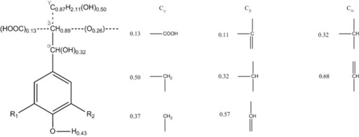
(a) Proposed structures of organosolv beech wood lignin units (H unit: R₁=R₂=H; G unit: R₁=H, R₂=OCH₃; S unit: R₁=R₂=OCH₃). (b) Possible configurations of the side chains and their occurrence.

The molar percentage of H, G, and S units in our lignin sample was calculated as 1.37, 43.26, and 55.37 %, respectively, based on NMR analysis of the methoxyl groups. From the structures given in Figure 1 and the abundance of H/G/S, the lignin overall formula was determined as C₉H_7.84O_2.34(OCH₃)_1.54. The amount of hydrogen is slightly over‐estimated, and can be explained by the fact that side‐chain cleavage (C_β or C_γ elimination) is not taken into account in the representative structure. Thus, it can be concluded that the two formulas derived from elemental and structural analyses are compatible, which validates the structures we propose in Figure 1.

Besides the proposed configuration, there might be other structures such as ketones, α‐O‐4 linkages, and α–α linkages, which are not taken into consideration in this work owing to their low signals intensities in the NMR spectrum. Moreover, the secondary aliphatic alcohol is the total amount of hydroxyl groups attached to C_α and C_β. However, to simplify our calculations, all the hydroxyl groups in the proposed structure were assigned to C_α, which makes an insignificant difference to the calculation of the solubility parameter.

Table 1 summarizes the calculation of the δ‐values. The correction factor Δv _correction in Equation (2) is calculated with n=9 (one phenylpropane unit). The δ‐values obtained for the H, G, and S lignin units are 26.4, 25.8, and 25.3 MPa^1/2, respectively. From the molar percentage, the overall Hildebrand solubility parameter for beech wood organosolv lignin is 25.5 MPa^1/2. The δ‐value of our organosolv lignin is comparable to those reported earlier such as the ALCELL® lignin from mixed hardwood (28.0 MPa^1/2),16 lignin obtained from enzymatic hydrolysis/mild acidolysis of bagasse (28.6 MPa^1/2),17 or the lignin from hydrolyzed almond shell (29.9 MPa^1/2).18

Table 1.

Calculation of the δ‐value of beech wood organosolv lignin from the proposed structures (Figure 1) using Equation (3).

Unit (abd.[a])	Group	Amt.[b]	Δe i [J mol−1]	Σ(Δe i) [J mol−1]	Δv i [cm3 mol−1]	Σ(Δv i) [cm3 mol−1]	δ [MPa1/2]
H (1.37 %)	−OH	1.25	29 790	37 238	10	12.5	26.4
	−COOH	0.13	27 614	3590	28.5	3.7
	−CH3	0.37	4707	1742	33.5	12.4
	−CH2	0.5	4937	2469	16.1	8.1
	−CH	0.64	3431	2196	−1.0	−0.6
	−CH=	1.25	4310	5387	13.5	16.9
	−C=	0.11	4310	474	−5.5	−0.6
	di‐sub. Ph	1	31 924	31 924	52.4	52.4
	O	0.83	3347	2778	3.8	3.2
	Δv corr					18
	TOTAL			87 796		125.8
G (43.26 %)	−OH	1.25	29 790	37 238	10	12.5	25.8
	−COOH	0.13	27 614	3590	28.5	3.7
	−CH3	1.37	4707	6449	33.5	45.9
	−CH2	0.5	4937	2469	16.1	8.1
	−CH	0.64	3431	2196	−1.0	−0.6
	−CH=	1.25	4310	5387	13.5	16.9
	C=	0.11	4310	474	−5.5	−0.6
	tri‐sub. Ph	1	31 924	31 924	33.4	33.4
	O	1.83	3347	6125	3.8	7
	Δv corr					18
	TOTAL			95 851		144.1
S (55.37 %)	−OH	1.25	29 790	37 238	10	12.5	25.3
	−COOH	0.13	27 614	3590	28.5	3.7
	−CH3	2.37	4707	11 156	33.5	79.4
	−CH2	0.5	4937	2469	16.1	8.1
	−CH	0.64	3431	2196	−1.0	−0.6
	−CH=	1.25	4310	5387	13.5	16.9
	−C=	0.11	4310	474	−5.5	−0.6
	tetra‐sub. Ph	1	31 924	31 924	14.4	14.4
	O	2.83	3347	9473	3.8	10.8
	Δv corr					18
	TOTAL			10 3905		162.4
						Avg.	25.5

[a] abd.=abundance. [b] Amount of functional group/atom per lignin unit.

Hildebrand parameter of GVL/water binary mixture

The calculation of Δ$H\genfrac{}{}{0pt}{}{\mathrm{vap}}{298\mathrm{K}}$ assumes an application of thermodynamic models for the estimation of the liquid and the vapor enthalpies at low pressures (P ^α and P ^β). Usually, the models are not precise in the pressure–temperature ranges out of the conditions of the experimental data used for a model optimization. In our calculations, the UNIQUAC model was derived based on vapor–liquid equilibrium (VLE) and excess enthalpy experimental data for the binary systems at moderate temperatures (303–351 K).20 Therefore, in this work, Δ$H\genfrac{}{}{0pt}{}{\mathrm{vap}}{298\mathrm{K}}$ calculations are not free of uncertainties. However, in many cases, the vaporization enthalpy does not depend significantly on the temperature or the pressure. The enthalpy of vaporization calculated by two different methods can be compared in Table 2. The Hildebrand parameters obtained from Equation (4) and from the estimation of enthalpy of vaporization of the mixture at standard conditions (δ _Eq. (4) and δ _298K, respectively) are comparable.

Table 2.

Solubility measurements in ternary system of water (1)–GVL (2)–lignin (3).

x [a]	w [b]	ν[c]	MW	ρ mixture	T b	$H\genfrac{}{}{0pt}{}{\mathrm{vap}}{298\mathrm{K}}$	δ298K	$H\genfrac{}{}{0pt}{}{\mathrm{vap}}{\mathrm{Eq}.\left(4\right)}$	δEq. (4)
			[g mol−1]	[g cm−3]	[K]	[J mol−1]	[MPa1/2]	[J mol−1]	[MPa1/2]
1	1	1	100.12	1.049	481.5	52 999	22.7	54 802[d]	23.1
0.9	0.98	0.979	91.91	1.048	480.5	51 589	23.3	54 483	24
0.8	0.957	0.955	83.7	1.046	410.1	50 430	24.2	54 094	25.2
0.7	0.928	0.925	75.49	1.042	391.3	49 438	25.3	53 584	26.4
0.6	0.893	0.888	67.28	1.038	382.9	48 580	26.5	52 952	27.7
0.5	0.848	0.841	59.07	1.033	378.4	47 798	27.9	52 176	29.3
0.4	0.788	0.779	50.86	1.028	375.9	47 049	29.8	51 178	31.2
0.3	0.707	0.694	42.65	1.022	347.5	46 321	32.2	49 942	33.5
0.2	0.582	0.569	34.44	1.014	373.8	45 580	35.4	48 136	36.4
0.1	0.383	0.37	26.23	1.006	373.6	44 798	40	45 449	40.3
0	0	0	18.02	0.997	373.6	43 978	47.6	40 681[e]	45.6

[a] Molar fraction of GVL in the mixture. [b] Weight fraction of GVL in the mixture. [c] Volume fraction of GVL in the mixture. [d] Enthalpy of vaporization of pure GVL30 [e] Enthalpy of vaporization of pure H₂O31

The Hildebrand parameter is only a guideline to the selection of the solubility conditions. Therefore, the simple calculation of the Hildebrand parameter and enthalpy of vaporization based on pure compound enthalpies, as in Equation (4), is a sufficiently accurate approximation to the Hildebrand parameter calculations. Thus, only $\mathrm{H}\genfrac{}{}{0pt}{}{\mathrm{vap}}{\mathrm{Eq}.\left(4\right)}$ was used further in this work.

Based on the Hildebrand parameter theory, the maximum solubility occurs when the δ‐value of the GVL/water mixture is close to that of lignin. According to the data from Table 1 and 2, lignin exhibits maximum solubility in a solution containing approximately 92–96 wt % GVL (70–80 mol % GVL).

Water–GVL–lignin ternary diagram

A solubility map (Figure 2) for the water–GVL–lignin mixture was determined at ambient temperature (≈294.6 K). The map is a pseudo‐ternary diagram, in which a complex mixture of lignin polymer fragments is described as one pseudo‐compound. Moreover, the lignin fragments demonstrate a polydispersity and conformational solvomorphism, which makes the solubility determination and establishment of the solubility map even more challenging. Because of these lignin properties, only a qualitative description of the solubility borders is possible. This general guide for the solubility behavior of the lignin in mixed solvents can help us understand the main phenomena that affect the lignin solubility. Additionally, qualitative knowledge of the phase split regions is valuable for the development of lignin‐related processes.

Figure 2.

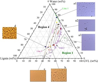
Ternary solubility map of water–GVL–lignin system at 294.6 K. Triangles indicate the compositions of split liquid phases. Crosses indicate the compositions at which the lignin agglomerations are visible in the homogenous region (region 1). Open circles indicate the compositions at which the liquid–liquid equilibrium occurs. Asterisks indicate the compositions at which solid–liquid–liquid equilibrium occurs. The dashed lines indicate the uncertainty in locating the borders. The microscopic images are magnified 40×.

Extension of the homogeneous regions and borders between the two‐ and three‐phase regions were obtained by visual inspection (Figure 2) of the formed phases using a microscope. Lignin prepared as described in the Experimental Section was virtually insoluble in water, whereas GVL could dissolve a substantial amount of the lignin. We prepared different lignin–GVL solutions with lignin content ranging from 0 to 55 wt % using 5 wt % increments. As the lignin content increased above 50 wt %, the solution became particularly viscous and solidified. Therefore, the maximum solubility of lignin in GVL at room temperature was assumed to be approximately 50 wt %.

A one‐phase region was found to exist along the water–GVL axis, which continued along the GVL–lignin axis until approximately 50:50 ratio of GVL/lignin (region 1, Figure 2). Microscopic examination revealed that lignin agglomerates exist in this phase at low GVL concentrations (Figure 2, image a1). As these lignin agglomerates cannot be separated by centrifugation, this phase can be considered as a colloidal sol mixture. At a relatively high water content in the mixture (>30 wt %) these agglomerates can form a solid phase (sub‐region T1, Figure 2). In this sub‐region, the precipitation of a relatively small amount of lignin can be triggered by the addition of water into the system, which destabilizes the colloidal lignin. Most of the remaining lignin remains in colloidal form (Figure 2, image a3). Upon further addition of water to the mixtures in the sub‐region T1, followed by ultrasonic mixing, the lignin precipitate re‐dispersed and stabilized in the colloidal form.

GVL and water are miscible at room temperature, but can form two separate liquid phases (liquid–liquid phase split, LLPS) in the presence of lignin to form an organic bottom phase with relatively high lignin concentration and an aqueous top phase with low lignin content (region 2, Figure 2). A splitting of the ternary water–GVL–lignin mixture to an organic and aqueous phase occurred at GVL concentrations between 30 and 50 wt %. The precise composition of the organic phase (line 2) could not be determined owning to the presence of water droplets in the organic phase, that is, an emulsion, even after 1 h of centrifugation (Figure 2, image b). Some of the organic phase also surrounded or was included in the lignin agglomerates in the aqueous phase (Figure 2, image a2).

Sub‐region T2 consisted of emulsions with a lignin concentration higher than that in the organic phase (line 3). Mixtures with a lignin content larger than 35 wt % were difficult to handle owing to high viscosity; it was usually impossible to distinguish between the solid and the organic phases. Water was dispersed as droplets in the pseudo‐organic phase (Figure 2, image c). After the addition of water, the water droplets increased in population and finally joined to form a separate water phase (region 2, Figure 2). Solvomorphism and the chemical structure of lignin are important factors in the formation of an emulsion. Therefore, the final state of the mixtures in this region depended on the lignin characteristics and on the preparation method of the mixture. Therefore, the estimation of the border of sub‐region T2 has some extent of uncertainty.

An increase in water or lignin content from the two‐phase region induced the precipitation of lignin and the formation of a solid–liquid–liquid split (SLLS) region (region 3, Figure 2). As both the aqueous and organic phases contained solid lignin particles, the precipitation started within the two‐liquid‐phase region (region 3 and region 2, Figure 2) and continued to region 4. In region 4, in which the lignin/GVL mass ratio is more than 1.5, GVL just wets the lignin particle surfaces and the organic phase is either not formed or consists of a high amount of lignin agglomerates (Figure 2, image d). The sub‐region T4 is a solid–liquid equilibrium region, in which a thick liquid phase of GVL (with a very small amount of dissolved water and ≈50 wt % of lignin) coexists with solid lignin.

The pseudo‐compound employed in this work demonstrated complicated phase behavior. A similar phase behavior was found for a much less complicated aqueous ternary system of butyl paraben in a mixture of water and ethanol, which has a phase diagram that resembles the lignin solubility map in this work.32, 33 Four solubility regions [one phase, liquid–liquid equilibrium (LLE), solid–liquid equilibrium (SLE), and solid–liquid–liquid equilibrium (SLLE)] were also observed in the work of Yang and Rasmuson33 at room temperature. Thus, it can be concluded that the monomeric unit of lignin, which resembles that of butyl paraben, behaves in a similar manner in the water–organic solvent mixture.

In industrial processes, a phase split significantly change the nature of the process. The presence of two liquid phases can suppress the growth of the lignin agglomerates. Both the formation of an emulsion and the liquid–liquid phase split prevent the precipitation of the undissolved lignin. However, the presence of the second phase can be useful for controlling the growth of lignin agglomerates33 and surface properties of the lignin particles. The low molecular weight lignin can be formed in the organosolv process,34 and its surface properties vary depending on the presence of the second liquid phase.

The behavior of lignin in GVL/water mixtures is different to those reported in previous works using mixed solvents (ethanol/water16 or 1,4‐butanediol/water17). Alcohols form a homogenous liquid phase with water at any concentration and lignin content, and the solubility of lignin increases exponentially with increasing molar ratio of the organic solvent. A maximum solubility is reached at a high concentration of the organic solvent, after which the solubility slightly decreases. The phenomenon is more complicated for the ternary water–GVL–lignin system, in which the solubility corresponds to points along the liquid phase regions. The solubility of lignin in mixtures with low GVL concentrations is insignificant (Figure 2, line 1), and increases slowly with higher GVL concentration up to 32 wt %. Above this concentration, the mixtures are split into two liquid phases and the overall solubility increases significantly (Figure 2, line 2). The sol aqueous phase shows a higher lignin solubility than before the phase split (Figure 3), owing to the inclusion of lignin agglomerates surrounded by the organic phase (Figure 2, image a2) which are well‐dispersed in the aqueous phase. The organic phase contains a significantly higher amount of lignin. With the addition of lignin to a mixture containing more than 60 % of GVL, the solid and organic phases are indistinguishable (sub‐region T2, region T4, and the lower part of region 1, Figure 2). The solubility cannot be determined precisely in such regions, indicated by the uncertainty in the determination of the phase region border (dashed line, Figure 2).

Figure 3.

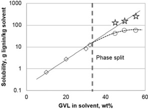
Solubility of lignin in GVL/water solution at room temperature. The diamonds denote the experimentally verified solubility in the aqueous phase (mixtures containing less than 32 wt % GVL), the circles indicate the total solubility of lignin in the sol aqueous phase, and the stars indicate the total solubility in the two‐phase region.

Application of the solubility diagram in GVL/water biomass fractionation

The calculated optimum GVL concentration for lignin dissolution based on the Hildebrand solubility parameter theory (92–96 wt %) fits quite well to the ternary solubility map (Figure 2, region 1; the lignin content in the ternary mixture drops significantly if the water content is more than 10 %). Information from the solubility map can be applied for the selection of operating parameters for a GVL/water biorefinery. A higher GVL concentration in the fractionation liquid promotes a higher driving force for lignin dissolution. However, biomass delignification is a more complicated process in which lignin first needs to be liberated from the biomass matrix by hydrolytic cleavage of the ether bond in the lignin–carbohydrate complex or between the lignin moieties. At an elevated temperature, water facilitates the cleavage of the acetyl group in hemicellulose, forming acetic acid.35 In turn, this creates the acidic medium that promotes the above‐mentioned hydrolytic activities. A balance between lignin liberation and dissolution must be reached. The GVL content should not exceed a level at which lignin fragmentation discontinues, but should also not be too low to diminish the dissolution of lignin. This fact was proven practically in the work by Fang et al.,36 in which birch (another type of hardwood) sawdust was treated at an elevated temperature in GVL/water mixtures of different concentration, with a liquor/wood ratio (L/W) of 10 L kg⁻¹. As mentioned earlier, pure GVL can dissolve an equal amount of lignin (i.e., 50 % lignin solution); however, it does not promote delignification owing to the absence of the hydrolytic cleavage reaction.36 The greatest extent of delignification was found at a GVL concentration between 50 and 65 wt %, well below the optimum solubility concentration determined in this work. Provided that the birch sawdust used in Fang's work contained 24 wt % lignin, the theoretical maximum lignin concentration in the spent liquor (provided that all lignin is extracted from the biomass) is about 2.4 wt %. At room temperature, a solvent containing 50 and 65 wt % GVL can dissolve 12 wt % and 23 wt % of lignin, respectively (line 2, Figure 2). The solubility is absolutely higher at a fractionation temperature above 160 °C. Therefore, using a 50–65 wt % GVL solution provides enough driving force for lignin dissolution and the remaining water content promotes adequate hydrolytic lignin fragmentation.

Even though the information from lignin solubility in GVL/water cannot be directly applied to the selection of the optimum fractionation liquor concentration, it can be applied in the processing of the spent liquor, the lignin‐containing liquid fraction obtained from the fractionation. Lignin can be precipitated from the spent liquor by the addition of water. The solubility of lignin significantly drops if the GVL concentration is below 35–40 wt % (region 1, Figure 2). Therefore, if lignin is extracted from biomass with a 50 wt % GVL in water, the addition of an equal amount of water would result in a liquid with approximately 25 wt % GVL, which has a considerably lower lignin solubility, leading to precipitation of a significant amount of lignin. This phenomenon can be used as a clean and effective method for lignin separation.

Efficient recovery of solvent and valorization of the dissolved products in spent liquor are important issues for the techno‐economic feasibility of a biorefinery concept. As discussed earlier, the L/W of 10 L kg⁻¹ employed in the work of Fang et al. was adequate to dissolve a major part of the birch lignin. Therefore, a lower L/W ratio can be considered to reduce the amount of liquid to be handled in the process, thus increasing the lignin concentration in the spent liquor and improving the practicality of the lignin recovery process. Remarkably, if L/W is adequately reduced, the spent liquor could experience spontaneous phase separation. Luterbacher et al. previously reported an effective chemical recovery pathway employing the liquid–liquid phase split phenomenon,15 in which phase separation of the spent liquor was induced by the addition of supercritical CO₂ or NaCl. The use of high pressure or inorganic salt can be replaced by spontaneous phase separation of the spent liquor. Lowering the L/W would bring the composition of the spent liquor from region 1 (homogeneous region) towards the lower left corner (lignin region, Figure 2). Phase separation occurs upon crossing the LLE border (line 2, Figure 2, equivalent to a lignin content of 13–21 wt % with 50–60 wt % GVL solvent). This phenomenon results in a lignin‐lean aqueous phase and a lignin‐rich organic phase (similar to the earlier discussion on the tie‐lines in region 2 and region 3, Figure 2), thus enabling an easy recovery of the spent liquor components. Phase separation also occurs if the spent liquor is cooled to room temperature, as the high fractionation temperature (typically>160 °C) facilitates the lignin dissolution, thus delaying the phase separation.

Conclusions

The Hildebrand solubility parameters were determined for both the solute beech wood organosolv lignin and different GVL/water solvent mixtures to predict the GVL/water mass ratio for the optimum solubility of the lignin. A simplified scheme was suggested for the Hildebrand parameter calculation of the mixed solvent. The Hildebrand parameter of lignin was estimated using an additive group contribution scheme. The optimum GVL concentration for lignin dissolution was predicted to be about 92–96 wt %, which agrees with the ternary solubility diagram of water–GVL–lignin. Two‐phase split region borders were found at 30–40 wt % of GVL in the mixture, which complicates the phenomenon and invalidates the definition of solubility in the mixed solvent. Besides the formation of a sol colloidal mixture of lignin in water, the formation of a water emulsion in GVL in the presence of lignin was confirmed by microscopic observations.

Despite the complicated behavior of lignin in GVL/water system, the results of this study support the feasibility of lignin isolation by the addition of water to the spent liquor. Furthermore, the spontaneous phase separation of the spent liquor induced by the reduction of the liquor/wood (L/W) ratio can be the basis for a commercially viable chemical recovery pathway.

Experimental Section

Materials

GVL (≥98 wt %, Sigma—Aldrich) was used for experiments in which the GVL concentration was less than 98 wt %. GVL was distilled to a purity of 99.9 wt % (confirmed by GC) for experiments that required a higher purity of GVL. The water content of distilled GVL was determined by Karl–Fischer titration (Mettler‐Toledo DL38, hydra point titrant 2 mg H₂O/mL and hydra point solvent G). Pure water (resistivity of 18.2 MΩ cm⁻¹) was produced on site using a Millipore Synergy® UV purification system.

Beech wood lignin samples, prepared by an organosolv fractionation process with ethanol/water, were supplied by Fraunhofer Center for Chemical and Biotechnological Processes.10 Lignin was ground manually with ceramic mortar and pestle and screened using a sieve with a 400 μm mesh, and the finer lignin fraction was employed in the experiment. Before solubility experiments, lignin was dried at 40 °C for 2 d and stored in a desiccator. Fine chemicals for the lignin analyses were supplied by Sigma–Aldrich and Merck.

Lignin characterization

The elemental analysis of lignin was performed with a FlashEA 1112 elemental analyzer series CHNS/O with a MAS200R autosampler (Thermo Fisher Scientific). The amount of methoxy groups in the lignin was determined in accordance with the Zeisel–Vieböck–Schwappach method.22

The carbohydrate (pentoses and hexoses) and lignin (acid soluble lignin and acid insoluble lignin) content of the lignin samples was analyzed in accordance with the two‐step hydrolysis method described in the NREL/TP‐510‐42618 standard. The first hydrolysis was performed with 10 mL of 72 % H₂SO₄ per gram of material at 30±3 °C for 60±5 min. The second hydrolysis step was performed with 300 mL of 4 % H₂SO₄ per gram of material at 121±1 °C for 60 min. The monosaccharides in the hydrolysate were analyzed using a high‐performance anion‐exchange chromatography (HPAEC) system (Dionex ICS‐3000; CarboPac PA20 column; pulsed amperometric detection, PAD). Acid‐insoluble lignin was determined gravimetrically whereas acid‐soluble lignin was determined from the absorbance at a wavelength of 205 nm (Shimadzu UV‐2550 spectrophotometer). As lignin was extracted from beech, a hardwood species, an extinction coefficient of 110 L/(g cm⁻¹) was the basis for quantification.23

The molecular mass distribution (MMD) of lignin was obtained by gel‐permeation chromatography (GPC) using a UV detector (UV/Vis Detector 2487). Dimethyl sulfoxide (DMSO) containing 0.1 % LiBr was used as a column eluent (1 mL min⁻¹ flow rate). The GPC system consisted of two analytical columns (Suprema 1000 and Suprema 100, 20 μm, 8 mm I.D. ×300 mm length) and one pre‐column (Suprema 20 μm, 9 mm I.D.×50 mm). The columns, injector, and UV detector were maintained at 80 °C during the analysis.

The content of the structural groups (hydroxyl, β‐O‐4) in the beech wood organosolv lignin was analyzed using NMR spectroscopy (Varian Unity Inova 500, 5 mm broadband probe head at 27 °C and 500 MHz ¹H frequency). Lignin samples were acetylated in pyridine/acetic anhydride mixture (1:1 by volume), purified with ethanol, and subsequently freeze‐dried.24 The sample for NMR analysis was dissolved in deuterated chloroform (CDCl₃) containing 0.03 % tetramethylsilane at a concentration of 150 mg mL⁻¹. For quantitative ¹³C experiments, inverse gated ¹H‐decoupling and 30° excitation pulse flip angle were utilized. The spectral width was 36 182.7 Hz, the relaxation delay was 5 s, and the acquisition time was 0.2 s. The number of transients varied between 41 215 and 49 683. Free induction decays were apodized using an exponential multiplication with 10 Hz line broadening and zero filled up to 16 384 complex points prior to Fourier transformation. For ¹³C experiments, the samples were doped with chromium(III) acetylacetonate (Cr(acac)₃) as a relaxation agent at a concentration of 10 mm.

The NMR spectrum of beech wood organosolv lignin is shown in the Supporting Information. The assignment of the resonance signals and their integration for quantification of the functional groups was performed in accordance with the method reported by Alekhina et al.25 The properties of the organosolv lignin are summarized in the Table 3.

Table 3.

Characterization of the beech wood organosolv lignin.

Property	Value
weight average molar mass [g mol−1]	3433
carbon [wt %]	62.54
hydrogen [wt %]	5.91
nitrogen [wt %]	0.25
oxygen [wt %]	30.85
ash [wt %]	0.05
hexose carbohydrate [wt %]	0.32
pentose carbohydrate [wt %]	1.90
acid soluble lignin [wt %]	1.65
acid insoluble lignin [wt %]	88.56
methoxyl group (OCH3) [wt %]	23.94
OCH3/C9 [a]	1.54
H/G/S[b]	1.4:43.2:55.4
primary aliphatic OH/C9 [c]	0.50
secondary aliphatic OH/C9 [c]	0.32
phenolic OH/C9 [c]	0.43
β‐O‐4/C9	0.26
−COOH/C9 [d]	0.13

[a] Number of methoxyl group per C₉ (phenylpropane unit). [b] Relative amount of lignin moieties p‐hydroxyphenyl (H)/guaiacyl (G)/syringyl (S). [c] Number of hydroxyl groups per phenylpropane unit. [d] Number of carboxylic groups in the aliphatic chain per phenylpropane unit.

Solubility of organosolv lignin in GVL/water binary mixtures

We predicted the solubility of lignin in GVL/water solvents based on the solubility parameter (δ‐value) theory, applicable to non‐polar and slightly polar systems.19, 26 Generally, a polymer, in this case, lignin, exhibits better solubility in a solvent with a δ‐value similar to that of lignin.19

The Hildebrand parameter of organosolv lignin

One classical approach for determining the δ‐value of a polymer includes determining the equilibrium swelling of a crosslinked polymer in a variety of solvents that have a wide range of δ‐values. The extent of swelling maximizes when the δ‐value of the solvent matches that of the polymer.27 Another approach is to measure the intrinsic viscosity of an uncrosslinked polymer in a series of solvents. The δ‐value for the polymer is taken to be the same as that of the solvent in which the polymer shows maximum viscosity.28

The above mentioned indirect methods are useful but tedious. In our case, we employed a more convenient method to estimate the δ‐value of polymer based on the additive contribution of atomic and functional groups present in the repeating unit structures,29 as shown in Equation (1).

$${\displaystyle \delta =\sqrt{\frac{\sum \left(\Delta e_i\right)}{\sum \left(\Delta v_i\right)}},}$$ (1)

where Δe _i is the additive atomic and functional group contributions for the energy of vaporization, Δv _i is the additive atomic and functional group contributions for the molar volume. The values for Δe _i and Δv _i were collected and tabulated by Fedors (1974).29 For high molecular weight polymers possessing a glass transition temperature greater than 25 °C, such as lignin, divergence in the molar volume is taken into account by the introduction of a correction factor,29 as in Equation (2).

$${\displaystyle \Delta v{}_{corr}=4n,n<3\Delta v{}_{corr}=2n,n\ge 3,}$$ (2)

where n is the number of main chain skeletal atoms in the smallest repeating unit of the polymer.

Hildebrand parameter of GVL/water binary mixtures

Schuerch suggested a method to calculate the solubility parameter of a low molecular weight liquid,26 as shown in Equation (3).

$${\displaystyle \delta =\sqrt{\frac{\Delta H^{vap}-\mathrm{R}{T}_b}{\mathrm{MW}}\times \rho },}$$ (3)

where δ is the solubility parameter (MPa^1/2), ΔH ^vap is the enthalpy of vaporization (J mol⁻¹), R=8.3144598 J/(K mol⁻¹), T _b is the boiling point of the mixture (K), ρ is the density (g cm⁻³) of the mixture, and MW is the average molecular weight (g mol⁻¹) of the mixture.

The densities of the GVL/water mixtures were adopted from the work of Zaitseva et al.20 and the boiling points of the mixtures were estimated using the UNIQUAC model for the fixed molar composition of a liquid and vapor phase. The Soave–Redlich–Kwong equation of state was used for modeling the vapor phase. In accordance with the Hildebrand theory, the Hildebrand parameter reflects the energy per volume consumed to break the interactions between the molecules in the liquid state.19 Thus, the Hildebrand parameter for the mixed solvent can be calculated from the pure solvent parameters (δ _i) and the solvent volumetric fractions (ν _i) (δ _mix=ν _GVL δ _GVL+ν _water δ _water), assuming that the change of the interaction energy owing to solvent mixing is negligible. This equation can be rewritten using the weight fraction (w_i) of the solvents in the mixture and their vaporization energy, as shown in Equation (4).

$${\displaystyle \Delta H^{\mathrm{vap}}=w_{\mathrm{GVL}}\frac{\rho }{{\rho }_{\mathrm{GVL}}}+w_{\mathrm{water}}\frac{\rho }{{\rho }_{\mathrm{water}}}\Delta H_{\mathrm{water}}^{\mathrm{vap}}}$$ (4)

Another approach used to calculate the solvent Hildebrand parameter is to estimate the enthalpy of vaporization of the mixture at standard conditions (298.15 K, Δ$H\genfrac{}{}{0pt}{}{\mathrm{vap}}{298\mathrm{K}}$ ). Theoretically, this approach provides an accurate estimation of the molecular interactions in the liquid state. In practice, this method is comparable with the calculations by Equation (4) because of various assumptions made for the calculation of the mixed solvent enthalpy of vaporization (Δ$H\genfrac{}{}{0pt}{}{\mathrm{vap}}{\mathrm{mix}}$ ). For the pure solvent, ΔH ^vap can be estimated from the solvent vapor pressure. However, for the mixed solvent, Δ$H\genfrac{}{}{0pt}{}{\mathrm{vap}}{\mathrm{mix}}$ depends on the interactions between different solvent molecules. The composition of the liquid changes when the mixtures boil. The boiling pressure or temperature also change, as indicated by the dashed line in Figure 4, or in the vapor–liquid equilibrium (VLE) diagram reported by Zaitseva et al.20 The composition of the vapor obtained from boiling of the mixture differs from the composition of the liquid. Therefore, Δ$H\genfrac{}{}{0pt}{}{\mathrm{vap}}{298\mathrm{K}}$ cannot be estimated at a fixed temperature and pressure. A preferable way to estimate Δ$H\genfrac{}{}{0pt}{}{\mathrm{vap}}{298\mathrm{K}}$ is to compare the total enthalpy of the liquid and vapor phases at a fixed temperature and composition but at a different pressure. This isothermal process is schematically shown in Figure 4, in which the evaporation of the liquid of composition x _GVL occurs owing to the reduction of the pressure from P ^α to P ^β at a constant temperature T=298 K. The temperature influences the total enthalpy of the phases considerably and should be kept constant.

Figure 4.

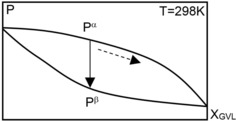
Estimation of the enthalpy of vaporization of a mixed solvent in the isothermal process.

Construction of the Water–GVL–lignin ternary diagram

To monitor the phase behavior of the ternary mixture of water–GVL–lignin, several three‐component mixtures were prepared in 15 mL Corning Pyrex® glass centrifugation tube. Ultrasonic mixing (ultrasonic bath VWR USC 200–2600) for approximately 2 h was employed to ensure the dissolution equilibrium. The mixture was incubated at an ambient temperature (≈294.5 K) for at least 7 h. The selection of a 7‐hour waiting time was not based on dissolution kinetic but on practical implications of this research. The water–GVL–lignin mixture is equivalent to the spent liquor in a biomass fractionation process, and the lifetime of the spent liquor in the process is typically less than 7 h; therefore, a longer waiting time is not necessary. The settlement of undissolved lignin was assisted by centrifugation for 60 min at 2100 g relative centrifugal force (Heraeus Sepatech Megafuge 1.0 centrifuge). Phase separation was determined visually and verified with a Leica DM750 polarizing microscope.

The solubility measurements started with binary mixtures of different concentrations followed by the addition of the third component and then the analysis of the obtained mixtures. An overview of the experiments is provided in Table 4. Each experiment was performed in triplicate. For measurements in which two liquid phases were formed, the compositions of the two coexisting liquid phases were determined by a combination of GC analysis and UV analysis.

Table 4.

Solubility measurements in a ternary system of water (1)–GVL (2)–lignin (3).

Starting mixture	Original compositions	Add. of 3rd component	Phenomena and analysis of the results
water (1)+GVL (2)	water content: 10–60 wt % with increment of 10 wt %	lignin: 16–250 mg per addition	liquid‐liquid equilibrium (LLE) concentration of lignin that caused the liquid–liquid split is calculated as the average of the amount of lignin added just before and after the phase separation.[a]
water (1)+GVL (2)	water content: 62, 64, 66, 68, 70, 80, 90 wt %[b]	lignin: 66–350 mg per addition	solid–liquid equilibrium (SLE) and LLE undissolved lignin was filtered (porosity 4 ROBU glass filter), dried at 105±5 °C and its weight was determined; dissolved lignin concentration was determined by UV spectrometer (Shimadzu UV‐2550, absorption at 280 nm with an extinction coefficient of 17.7 L g−1 cm−1).[c]
GVL (2)+lignin (3)	lignin content: 5–55 wt %[c,d] with increment of 5 wt %	water: 100–500 mg per addition	SLE and LLE the concentration of water that caused the lignin precipitation is calculated as the average of the amount of water added just before and after the precipitation.[a]

[a] The uncertainty of the concentration determination is equal to half of the concentration change between two consecutive additions of the third component. [b] A fine increment from 60 to 70 wt % is owing to the phase split observation in this region. [c] The mass balance of lignin was on average within 2 % of error. [d] The solution is too viscous to be handled at concentrations of lignin in GVL above 55 wt %.

In GC analysis, 0.5 mL of a one‐phase sample was dissolved in 0.9 mL dried acetone and 1 μL of the mixture was injected into GC using a liquid sampler (Agilent 7683). Solid particles were separated from the analyzed mixture in the liner of the GC inlet (collected by the liner glass wool). A polar capillary column (DW‐WaxETR, Agilent 30 m×0.320 mm×1 μL) was used to separate the injected liquid, and the outlet compounds were analyzed by a thermal conductivity detector (TCD, 523.15 K, reference helium flow 25 mL min⁻¹). The helium flow in the GC column was 1.6 mL min⁻¹ and the GC oven temperature started at 353.15 K for 2 min and was raised to 443.15 K at a heating rate of 50 K min⁻¹ rate and held for 3 min and raised again to a final temperature of 483 K, which was held for 3 min. A good separation between the GVL and water was achieved and an accuracy of 0.2 % of the GVL/water concentration was confirmed by calibrating the TCD detector with gravimetrically prepared binary mixtures. Thus, the relative amount of the water and GVL in the samples was determined.

The lignin content of one‐phase samples was analyzed by UV/Vis spectrophotometry. approximately 9–37 mg of the samples was diluted with 35 wt % solution of aqueous ethanol to either 25 or 50 mL (the amount of sample diluted and the dilution depended on the lignin concentration). The lignin concentration was calculated from the absorption at a wavelength of 280 nm using the extinction coefficient of 17.7 L g⁻¹ cm⁻¹), which was measured for the lignin sample used in this study in the calibration of the Shimadzu UV‐2550 spectrometer (Supporting Information).

Supporting information

As a service to our authors and readers, this journal provides supporting information supplied by the authors. Such materials are peer reviewed and may be re‐organized for online delivery, but are not copy‐edited or typeset. Technical support issues arising from supporting information (other than missing files) should be addressed to the authors.

Supplementary

H. Q. Lê, A. Zaitseva, J.-P. Pokki, M. Ståhl, V. Alopaeus, H. Sixta, ChemSusChem 2016, 9, 2939.

References

- 1. Balan V., Chiaramonti D., Kumar S., Biofuels Bioprod. Biorefin. 2013, 7, 732–759. [Google Scholar]
- 2. Huber G. W., Iborra S., Corma A., Chem. Rev. 2006, 106, 4044–4098. [DOI] [PubMed] [Google Scholar]
- 3. Sjöström E., Wood chemistry: Fundamentals and applications, Academic Press, San Diego, 1993. [Google Scholar]
- 4. Iakovlev M., Pääkkönen T., van Heiningen A., Holzforschung 2009, 63, 779–784. [Google Scholar]
- 5. Dutta S., Pal S., Biomass Bioenergy 2014, 62, 182–197. [Google Scholar]
- 6. Gürbüz E. I., Gallo J. M. R., Alonso D. M., Wettstein S. G., Lim W. Y., Dumesic J. A., Angew. Chem. Int. Ed. 2013, 52, 1270–1274; [DOI] [PubMed] [Google Scholar]; Angew. Chem. 2013, 125, 1308–1312. [Google Scholar]
- 7. Mellmer M. A., Martin Alonso D., Luterbacher J. S., Gallo J. M. R., Dumesic J. A., Green Chem. 2014, 16, 4659–4662. [Google Scholar]
- 8. Pye E. K., Lora J. H., Tappi J. 1991, 74, 113–118. [Google Scholar]
- 9. Kleinert T. N., Tayenthal K., US1856567A, 1932.
- 10. Laure S., Leschinsky M., Froehling M., Schultmann F., Unkelbach G., Cellul. Chem. Technol. 2014, 48, 793–798. [Google Scholar]
- 11. Horváth I. T., Green Chem. 2008, 10, 1024–1028. [Google Scholar]
- 12. Emel′yanenko V. N., Kozlova S. A., Verevkin S. P., Roganov G. N., J. Chem. Thermodyn. Thermochem. 2008, 40, 911–916. [Google Scholar]
- 13. Horváth I. T., Mehdi H., Fabos V., Boda L., Mika L. T., Green Chem. 2008, 10, 238–242. [Google Scholar]
- 14. Alonso D. M., Wettstein S. G., Mellmer M. A., Gurbuz E. I., Dumesic J. A., Energy Environ. Sci. 2013, 6, 76–80. [Google Scholar]
- 15. Luterbacher J. S., Rand J. M., Alonso D. M., Han J., Youngquist J. T., Maravelias C. T., Pfleger B. F., Dumesic J. A., Science 2014, 343, 277–280. [DOI] [PubMed] [Google Scholar]
- 16. Ni Y., Hu Q., J. Appl. Polym. Sci. 1995, 57, 1441–1446. [Google Scholar]
- 17. Wang Q., Chen K., Li J., Yang G., Liu S., Xu J., BioResources 2011, 6, 3034–3043. [Google Scholar]
- 18. Quesada-Medina J., López-Cremades F. J., Olivares-Carrillo P., Bioresour. Technol. 2010, 101, 8252–8260. [DOI] [PubMed] [Google Scholar]
- 19. Hildebrand J. H., Scott R. L., The solubility of nonelectrolytes, Rheinhold, New York, 1950. [Google Scholar]
- 20. Zaitseva A., Pokki J., Le H. Q., Alopaeus V., Sixta H., J. Chem. Eng. Data 2016, 61, 881–890. [Google Scholar]
- 21.Aspen Technology 2015, Aspen Plus 8.6, http://www.aspentech.com/products/engineering/aspen-plus/.
- 22. Zakis G. F., Functional analysis of lignins and their derivatives, TAPPI PRESS, Atlanta (GA), 1994. [Google Scholar]
- 23. Swan B., Sven. Papperstidn. 1965, 68, 791–795. [Google Scholar]
- 24. Lin S. Y., Dence C. W., Methods in lignin chemistry, Springer, 1992, pp. 578–581. [Google Scholar]
- 25. Alekhina M., Ershova O., Ebert A., Heikkinen S., Sixta H., Ind. Crops Prod. 2015, 66, 220–228. [Google Scholar]
- 26. Schuerch C., J. Am. Chem. Soc. 1952, 74, 5061–5067. [Google Scholar]
- 27. Gee G., Inst. Rubber Ind. 1943, 18, 266. [Google Scholar]
- 28. Gardon J. L., Encyclopedia of Polymer Science and Technology, Wiley, New York, 1965. [Google Scholar]
- 29. Fedors R. F., Polym. Eng. Sci. 1974, 14, 147–154. [Google Scholar]
- 30. Alonso D. M., Wettstein S. G., Dumesic J. A., Green Chem. 2013, 15, 584–595. [Google Scholar]
- 31. Perry R. H., Green D. W., Handbook Perry′s Chemical Engineering, 7th Edition, McGRAW-HILL, USA, 1997. [Google Scholar]
- 32. Yang H., Rasmuson Å. C., Org. Process Res. Dev. 2012, 16, 1212–1224. [Google Scholar]
- 33. Yang H., Rasmuson Å. C., Fluid Phase Equilib. 2015, 385, 120–128. [Google Scholar]
- 34. Veesler S., Revalor E., Bottini O., Hoff C., Org. Process Res. Dev. 2006, 10, 841–845. [Google Scholar]
- 35. Brasch D. J., Free K. W., Tappi 1965, 48, 245–248. [Google Scholar]
- 36. Fang W., Sixta H., ChemSusChem 2015, 8, 73–76. [DOI] [PubMed] [Google Scholar]
Associated Data
This section collects any data citations, data availability statements, or supplementary materials included in this article.
Supplementary Materials