

Abstract
Although it is currently best-practice to directly model latent factors whenever feasible, there remain many situations in which this approach is not tractable. Recent advances in covariate-informed factor score estimation can be used to provide manifest scores that are used in second-stage analysis, but these are currently understudied. Here we extend our prior work on factor score recovery to examine the use of factor score estimates as predictors both in the presence and absence of the same covariates that were used in score estimation. Results show that whereas the relation between the factor score estimates and the criterion are typically well recovered, substantial bias and increased variability is evident in the covariate effects themselves. Importantly, using covariate-informed factor score estimates substantially, and often wholly, mitigates these biases. We conclude with implications for future research and recommendations for the use of factor score estimates in practice.
Keywords: Factor score estimation, item response theory, moderated nonlinear factor analysis, integrative data analysis
Scientific progress depends on the development, refinement, and validation of measures that sensitively and reliably quantify the phenomena of theoretical interest. For instance, astronomers have made remarkable progress in recent years in exoplanetary research by precisely measuring the light produced by stars that reaches the Earth. Periodic dips in the light observed from a star signal the presence of an exoplanet, and can be used to determine its size and length of orbit. Differences in the dimming of different wavelengths can even be used to infer the presence and composition of an atmosphere, recently resulting in the identification of an Earth-like planet with a water-rich atmosphere (Southworth et al., 2017). Measurement plays an equally important role in the behavioral and social sciences. Similar to astronomical research, we typically must rely on measurements of observable characteristics of peripheral interest to infer the unobservable characteristic of more central theoretical concern. Just as astronomers use measurements of light wavelengths to infer the composition of an atmosphere that cannot be directly sampled, psychologists use self-reports of sadness, hopelessness, fatigue, and loneliness to infer the underlying level of depression of an individual.
Latent Variable Models
Latent variable measurement models constitute the primary analytic approach used in the behavioral and social sciences for measuring constructs that are not directly observable (e.g., depression) on the basis of observed indicator variables thought to reflect these constructs (e.g., self-reports of sadness and hopelessness). This broad class of latent variable models includes linear and nonlinear factor analysis, item response theory (IRT) models, latent class/profile models, structural equation models (SEMs), and many others. Despite more than a century of research on latent variable models dating back to Spearman (1904), debate still exists about how best to use these models to generate numerical measures of the underlying latent constructs of interest.
Lying at the root of the controversy is the issue of indeterminacy. Because latent variables are by definition unobserved, we cannot recover their values exactly from the observed indicator variables. Thus, the true values of the latent variables are indeterminate (e.g., Bollen, 2002; Steiger & Schönemann, 1978). As a consequence, a variety of approaches have been developed for scoring latent variables that optimize different criteria. For the linear factor analysis model, approaches for generating factor score estimates include the regression method (which minimizes the variance of the scores; Thomson, 1936; Thurstone, 1935), Bartlett’s method (which results in conditionally unbiased scores; Bartlett, 1937), and the Anderson and Rubin method (Anderson & Rubin, 1956, as extended by McDonald, 1981) which results in scores that replicate the covariances among the latent variables.
In modern treatments, the issue has been reframed in terms of how best to characterize the posterior distribution of the latent variable for a person given his or her set of responses to the observed indicator variables (Bartholomew & Knott, 1999), with the most common choices being the mode (modal a posteriori scores, or MAPs) and expected value (expected a posteriori scores, or EAPs). Notably, EAPs and MAPs are equivalent to one another and to regression method scores for normal-theory linear factor analysis, but generalize to other latent variable models, such as nonlinear factor analysis or item response theory models, where they are typically highly correlated but not identical in value. Given this plethora of ways to score latent variables, researchers (including us) are left with the daunting task of choosing which method is ideal for a given application, knowing that different methods may lead to different conclusions.
Contemporary Need for Scale Scores
Although the question of how best to score latent variables was once of critical concern, the development of structural equation modeling allowed many psychometricians and applied researchers to neatly sidestep the issue. Without ever having to generate scores, SEMs can produce direct estimates of the relationships between latent variables or between latent variables and directly observed predictors or criteria (e.g., Bentler & Weeks, 1980; Bollen, 1989; Jöreskog, 1973). Given this capability, many methodologists have advised against using scores, which vary depending on the method used to compute them and never perfectly measure the latent construct, in favor of using SEMs (e.g., Bollen, 2002). Indeed, this aversion to scores became so strong that one prominent (and wonderfully irreverent) psychometrician used his 2009 Psychometric Society Emeritus Lecture to bemoan the irony that latent variable measurement models were so infrequently being used to produce any actual measurements (McDonald, 2011).
Recent years, however, have seen a resurgence of interest in scoring methods, in part due to a variety of practical research needs. For example, some questions can only be addressed by scores, such as when interest centers on individual assessment or selection (e.g., Millsap & Kwok, 2004) or in propensity score modeling (e.g., Raykov, 2012). Further, large public datasets are analyzed in multiple ways by many users and, without the provision of scores, each user would face the responsibility of constructing measurement models anew (e.g., Vartanian, 2010). This task places a burden on users and presents the risk that different users will construct different measurement models, resulting in inconsistent results. However, simultaneous estimation of measurement and structural models within an SEM is often simply not tractable. For instance, in our own work, we have used score estimates in the context of combining longitudinal data sets for the purpose of conducting integrative data analysis (or IDA; Curran, 2009; Curran & Hussong, 2009; Hussong et al., 2007, 2008, 2010, 2012). Given the complexity of multiple studies each with different numbers of items and many repeated assessments, it was simply infeasible to fit a longitudinal measurement model and a growth model concomitantly. We thus computed scores and carried those scores into subsequent analyses, a strategy that has proven expedient for other applications IDA as well (e.g., Greenbaum et al., 2015; Rose, Dierker, Hedeker, & Mermelstein, 2013).
Thus in many situations commonly encountered in a broad range of research applications, the ultimate objective in generating scores is to substitute the scores for the latent variables in some form of second-stage analysis. That this purpose should therefore drive the determination of how to score latent variables optimally was first appreciated by Tucker (1971). Following this logic and focusing on the linear factor analysis model, Tucker demonstrated that the regression method is optimal when scores are to be used as predictors of other variables, whereas Bartlett scoring is optimal when scores are instead to be used as outcomes.
More recently, Skrondal and Laake (2001) updated Tucker’s original findings, proving that regression coefficient estimates are consistent when using regression method scores as predictors or Bartlett method scores as outcomes. Skrondal and Laake also extended Tucker’s results in several ways, for instance, showing that when factors are correlated, they should be scored simultaneously based on a multidimensional factor model rather than separately based on unidimensional models. Subsequently, Hoshino and Bentler (2013) developed a new scoring method that produces consistent estimates regardless of whether factor scores are used as predictors or outcomes, avoiding the awkwardness of computing differing scores for different purposes. Extending beyond the linear factor analysis model, Lu and Thomas (2008) showed that Skrondal and Laake’s core results also hold for nonlinear item-level factor analysis / IRT, where EAPs represent the generalization of regression method scores and produce consistent estimates of regression coefficients when used as predictors of observed criterion variables.
Inclusion of Covariates in Scoring
In addition to the work described above, another point of emphasis in the modern literature on scoring has been the value of incorporating information on background variables (i.e., covariates) when generating scores. Such variables may enter a latent variable measurement model in two ways. First, the covariates can have a direct impact on the distribution of the latent variable. For instance, Bauer (2017) conditioned both the mean and variance of a violent delinquency factor on age and sex, finding that boys displayed higher and more homogeneous levels of delinquency that decreased less rapidly over ages 12 to 18 than girls. Second, covariates can have direct effects on the observed indicators / items above and beyond their impact on the latent variable itself. Such effects produce differential item functioning (DIF), such that the same item responses are differentially informative about the latent variable depending on the background variable profile. In the same application, Bauer (2017) found that several items demonstrated DIF by age and/or sex. As one example, the item “hurt someone badly enough to require bandages or care from a doctor” was more commonly endorsed by boys, particularly at older ages, than would be expected based on sex and age differences in the delinquency factor alone. Such trends may reflect the growing capacity for the same behaviors to result in greater consequences as boys mature.
Recently, our group conducted an extensive simulation on the value of incorporating these two types of covariate effects, impact and DIF, into the measurement model used to generate factor scores (Curran et al., 2016). Focusing on EAPs, we showed that the correlation of the score estimates with the true underlying factor scores clearly increased when covariate effects were included in the measurement model, particularly when the covariates had greater impact on the factor mean. For example, across varying experimental conditions, the true score correlation when entirely omitting the covariates ranged from .75 to .92, when estimating only impact ranged from .77 to .93, and when estimating both impact and DIF ranged from .81 to .93. We expected these findings as the inclusion of informative covariates provided additional information from which to produce score estimates (i.e., increased factor determinacy that resulted in posterior score distributions with lower variance). However, we did not anticipate the finding that accounting for impact and DIF in the measurement model had only a small effect on the magnitude of the correlation between the EAPs and the true factor scores. There were distinct improvements in true score recovery with the inclusion of the covariates in the scoring model (see, e.g., Curran et al., 2016, Table 3), but the magnitude of these gains were at best modest and at times verging on negligible.
Table 3.
Population values for the three regression models.
| Regression Coefficient |
Squared Semi-partial Correlation | |||
|---|---|---|---|---|
| Outcome 1 () | SMLV | MMMV | LMSV | |
| Intercept | 10.16 | |||
| 1.07 | 0.166 | 0.166 | 0.166 | |
| 5.72 | ||||
| .17 | ||||
| Outcome 2 () | SMLV | MMMV | LMSV | |
| Intercept | 10.16 | |||
| 1.07 | 0.122 | 0.113 | 0.091 | |
| Age | 0.36 | 0.023 | 0.022 | 0.019 |
| Sex | 0.44 | 0.020 | 0.020 | 0.020 |
| Study | −1.24 | 0.115 | 0.108 | 0.090 |
| 5.72 | ||||
| .35 | ||||
| Outcome 3 () | SMLV | MMMV | LMSV | |
| Intercept | 10.16 | |||
| 1.07 | 0.094 | 0.085 | 0.065 | |
| Age | 0.36 | 0.020 | 0.019 | 0.016 |
| Sex | 0.44 | 0.017 | 0.017 | 0.018 |
| Study | −1.24 | 0.100 | 0.093 | 0.075 |
| Stress | 0.8 | 0.055 | 0.055 | 0.054 |
| 5.72 | ||||
| .43 | ||||
note: impact denoted SMLV=small mean, large variance; MMMV=medium mean, medium variance; LMSV=large mean, small variance; see text for details. = multiple r-squared; one value is listed for each outcome for conciseness, although these values vary slightly (by +/−.01) as a function of impact.
Given the rather small gains in true score recovery associated with the inclusion of the exogenous covariates, a logical question arises as to whether the added complexity of covariate-informed scoring procedures is worthwhile. However, to fully address this issue we must carefully consider the conditions under which the estimated scores are most commonly used; namely, as predictors or criteria in second-stage modeling procedures. In our prior work, we strictly focused on true score recovery. That is, we examined the extent to which the estimated factor scores corresponded to their underlying true counterparts. While this is a necessary step in establishing how the score estimates perform under conditions reflecting their use in practice, it is not sufficient in that we have yet to examine the relations between the scores and outcomes. As such, our current work follows Tucker’s (1971) admonition that estimated scores should be evaluated in relation to their intended purpose.
Factor Score Estimates as Predictors
Little is currently known about how to best use factor score estimates as predictors in second-stage models. Although understudied in the behavioral and health sciences, a small body of relevant research currently exists on this point within the educational measurement literature on plausible value methodology. In a key paper, Mislevy, Johnson and Muraki (1992) argued that the values of a latent variable can be viewed as missing, and thus that scoring procedures can be conceptualized as imputation methods for producing plausible realizations of the missing values. Within the missing data literature, best practice is to include in the imputation model (here, the latent variable measurement model) all variables that will feature in second-stage analyses, including other auxiliary variables (here, the exogenous covariates) that may be related to the missing values. Drawing on this parallel, Mislevy et al. (1992) argued that scores for latent variables should be based on a model that conditions the latent variable on relevant observed background variables.
The approach of Mislevy, however, allowed for only impact effects and not DIF, assuming that any items with DIF would have previously been identified and eliminated. Although this assumption was reasonable within the context of their research on large-scale educational testing, it is less realistic in many other research contexts where the pool of potential items for a given construct is often limited and removing items with DIF may result in failure to fully cover the content domain of the construct (Edelen, Stucky & Chandra, 2015). The focus then turns to mitigating the biases associated with DIF. A key goal of our paper is to investigate the performance of scores generated from measurement models that either include or omit impact and DIF when these scores are to be used in second-stage analyses.
The Current Paper
To investigate the need to include covariate effects in scoring models more thoroughly, we move beyond our prior simulation work presented by Curran et al. (2016) to consider the performance of covariate-informed scores in subsequent analyses. Specifically, under a variety of realistic conditions, we compute EAPs from three latent variable measurement models: one that excludes the covariates entirely, one that includes covariate impact but not DIF, and one that includes both impact and DIF. We then use the EAPs obtained from these three scoring models as predictors in a series of linear regression analyses. Based on the literature reviewed above, we made three primary hypotheses for how the different scores would perform in these analyses.
First, when score-based regression analyses include no other predictors but the scores, given a sufficient sample size, all three scoring methods will generate largely unbiased regression coefficient estimates; however, we did expect differences in variability (assessed via root mean squared error) across the three scoring models. Second, when score-based regression analyses include covariates in addition to the scores, it will be necessary to include the same covariates in the scoring model in order to obtain unbiased regression coefficient estimates; in contrast, excluding the covariates from the scoring model will result in meaningful bias. Third, when score-based regression analyses include covariates, using a scoring model that accounts for any DIF due to the covariates will be necessary to obtain unbiased regression coefficient estimates. Although Curran et al. (2016) found no notable difference in the correlations between the score estimates and true scores when models included versus excluded DIF, we speculated that excluding DIF from the scoring model might have more meaningful consequences for score-based analyses. Our reasoning was that failure to model DIF (when present) would lead to bias in covariate impact estimates thus distorting the correlations between the scores and the covariates; this in turn is expected to bias the partial regression coefficient estimates obtained from score-based analyses that include both the scores and the covariates.
Methods
Our motivating goal was to examine the recovery of predictor-criterion relations in models in which one of the predictors was estimated using various specifications of a latent variable scoring model. Although we selected design elements to mimic what might be encountered in an integrative data analysis setting (specifically, data pooled across two independent samples), our conditions and subsequent results directly generalize to single study designs as well. Because complete details relating to the data generation procedure for the factor scores and items are presented in Curran et al. (2016), we only briefly review these steps. Because the generation process for the outcome variables have not been presented elsewhere, we discuss these in greater detail.
Data Generation
We followed a four-step process to generate data consistent with a single factor latent variable model defined by a set of binary indicators that are differentially impacted by a set of exogenous covariates that in turn jointly influence three separate outcomes. The top panel of Figure 1 presents a conceptual path diagram of the population generating model. The diagram is simplified and intentionally imprecise to enhance clarity, and we provide specific equations for all models and outcomes below.
Figure 1. Conceptual path diagram of population model (top panel) and predictive regression model (bottom panel).
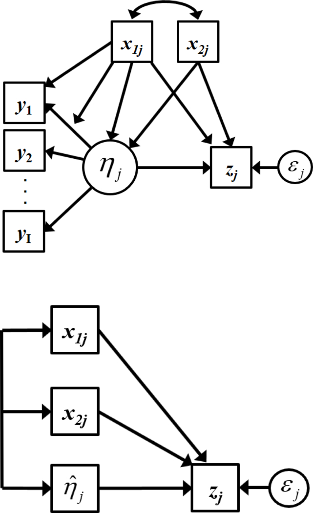
note: These are conceptual representations, the specifics of which are defined via equations in the text. In the top panel the arrows connecting the covariates to the measurement model represents impact (pointing to the latent factor) and DIF (pointing to the factor loading and item). The diagram shows two covariates for simplicity, but three and four covariates were used in the simulations.
Step 1: Exogenous covariates.
Exogenous covariates were generated for each simulated observation j to reflect variables that are common in an IDA design. The first three covariates were defined to exert both impact and DIF effects in the measurement model, and the fourth to covary with the latent factor but not be functionally related to impact or DIF. This fourth covariate was designed to reflect the commonly used approach in which a variable is not included in the measurement model but is included in subsequent fitted models.
More specifically, the first covariate was designed to mimic study membership (studyj) and was generated as a binary indicator with half of a given simulated sample drawn from Study 1 and half from Study 2. The second covariate was designed to mimic biological sex (sexj) and was generated from a Bernoulli distribution with probability of being a male equal to .35 in Study 1 and .65 in Study 2. The third covariate was designed to mimic chronological age (agej) and was generated from a binomial distribution with success probability of .5 over seven trials with ages ranging from 10 to 17 in Study 1 and over six trials with ages ranging from 9 to 15 in Study 2; the age range was shifted across study to reflect age heterogeneity that is common in real-world IDA applications. The fourth covariate was designed to mimic perceived stress (stressj) and was generated as a continuous covariate that correlated with the latent factor (r=.35) but was orthogonal to the first three predictors.
Step 2: Latent True Scores.
The latent factor was designed to mimic depression () and was generated from a continuous normal distribution with moments defined as a function of the three covariates. More specifically, the value of was randomly drawn from a normal distribution with mean αj and variance ѱj where the subscripting with j reflects that the mean and variance are expressed as deterministic functions of the covariates unique to observation j. Specifically, the mean of the latent distribution was defined as:
| (1) |
and the variance as:
| (2) |
where the coefficients for the latent mean (γ ‘s) and the latent variance (δ ‘s) jointly represent impact. The two equations include different covariate effects both to reflect what might be encountered in practice and to highlight that each parameter can be defined by a unique combination of the covariates.
Step 3: Observed items.
The observed binary items were designed to mimic the presence or absence of symptoms of depression (yij for item i and subject j) and were generated as a function of the three covariates and the true latent score. Specifically, binary responses were generated from a Bernoulli distribution with success probability μij given by:
| (3) |
where values of the item intercept (vij) and factor loading (λij) were functions of the covariates. The effect of the covariates on the item intercept was defined as:
| (4) |
and for the item slope (or loading) as
| (5) |
The coefficients for the intercept (κ ‘s) and the slope (ω ‘s) jointly define DIF.
Step 4: Outcomes.
Three outcomes, designed to represent hypothetically relevant measures such as school success, antisocial behavior, or self esteem (zmj) for outcome m and subject j), were generated according to one of three models. The bottom panel of Figure 1 presents a conceptual diagram of the regression models; this shows only one outcome, although three were considered. The first model (denoted Outcome 1) consisted of just the univariate effect of the true score :
| (6) |
The second model (denoted Outcome 2) added main effects of all of the DIF- and impact-generating covariates:1
| (7) |
The third and final model (denoted Outcome 3) added to the second model the additional covariate designed to mimic stress:
| (8) |
Design Factors
Five factors were manipulated as part of the experimental design: sample size, number of items, magnitude of impact, magnitude of DIF, and proportion of items with DIF. All factors were fully crossed yielding a total of 108 unique conditions for each of which 500 replications were generated.
Sample size.
We investigated three sample sizes: 500, 1000, and 2000. These sample sizes were evenly divided between the two simulated studies (e.g., for the n=500 condition, 250 cases were drawn from Study 1 and 250 from Study 2).
Number of items.
We investigated three numbers of observed items: 6, 12, and 24. These correspond to small, medium, and large item sets commonly seen in practice.
Latent variable impact.
We investigated three types of latent variable impact: small mean/large variance (SMLV), medium mean/medium variance (MMMV), and large mean/small variance (LMSV). Combinations of mean and variance impact parameters were chosen to produced the desired shift in latent variable mean and variance while holding the marginal variance of the latent variable equal across conditions. All population coefficients corresponding to Equations 1 and 2 are presented in Table 1.
Table 1.
Population values of covariate moderation three impact conditions.
| Small Mean / Large Variance |
Medium Mean / Medium Variance |
Large Mean / Small Variance |
|
|---|---|---|---|
| Mean Model | |||
| Intercept | −0.01 | −0.01 | −0.02 |
| Age | 0.13 | 0.22 | 0.34 |
| Gender | 0 | 0 | 0 |
| Study | 0.21 | 0.37 | 0.56 |
| Age × Study | −0.05 | −0.09 | −0.14 |
| Variance Model | |||
| Intercept | 0.58 | 0.71 | 0.65 |
| Age | 0.5 | 0.35 | 0.25 |
| Gender | −1 | −0.6 | −0.05 |
| Study | 0.5 | 0.3 | 0.05 |
DIF magnitude.
We investigated two levels of DIF magnitude: small and large. DIF magnitude was chosen on the basis of exploratory analyses, which included calculating the weighted area between curves (wABC; Edelen et al., 2015; Hansen et al., 2014) in order to quantify the difference between model-implied trace lines. All population coefficients corresponding to Equations 3 and 4 are presented in Table 2.
Table 2.
Population values of item parameters under small and large DIF conditions.
| Loading | Small DIF |
Large DIF |
|||||
| Baseline | Age | Gender | Study | Age | Gender | Study | |
| Items 1, 7, 13, 19 | 1 | ||||||
| Items 2, 8, 14, 20 | 1.3 | 0.05 | −0.2 | 0.2 | 0.075 | −0.3 | 0.3 |
| Items 3, 9, 15, 21 | 1.6 | −0.05 | 0.2 | 0.2 | −0.075 | 0.3 | 0.3 |
| Items 4, 10, 16, 22 | 1.9 | 0.05 | 0.075 | ||||
| Items 5, 11, 17, 23 | 2.2 | −0.2 | 0.2 | −0.3 | 0.3 | ||
| Items 6, 12, 18, 24 | 2.5 | ||||||
| Intercept | Small DIF |
Large DIF |
|||||
| Baseline | Age | Gender | Study | Age | Gender | Study | |
| Items 1, 7, 13, 19 | −0.5 | ||||||
| Items 2, 8, 14, 20 | −0.9 | 0.125 | −0.5 | 0.5 | 0.25 | −1 | 1 |
| Items 3, 9, 15, 21 | −1.3 | −0.125 | 0.5 | 0.5 | −0.25 | 1 | 1 |
| Items 4, 10, 16, 22 | −1.7 | 0.125 | 0.25 | ||||
| Items 5, 11, 17, 23 | −2.1 | −0.5 | 0.5 | −1 | 1 | ||
| Items 6, 12, 18, 24 | −2.5 | ||||||
Proportion of items with DIF.
We investigated two levels of proportion of items with DIF: 33% and 66% of items. In both the 33% and 66% DIF conditions, we generated a balance of negative and positive DIF effects between and within items to keep endorsement rates from becoming unreasonably low, and to mimic the compensatory pattern of DIF often seen in practice.
Outcome coefficients.
Whereas the values of coefficients for impact and DIF varied in magnitude across the experimental design (e.g., small, medium, large), the coefficients that defined the regression models for the three outcomes were held constant across varying conditions of impact and DIF. The population values were chosen to optimize three criteria: to maintain approximately equivalent R-squared values across the three impact conditions; to balance positive and negative effects of covariates to allow examination of differential bias as a function of the sign of the coefficient; and to reflect a range of magnitudes of effect that are typical of research applications in the behavioral and health sciences. Population values for all regression models are presented in Table 3 including the raw coefficients, squared semi-partial correlations, and the model R-squared.
Factor Scoring Models
We used three parameterizations of the latent variable model to obtain factor score estimates: an unconditional model, an impact-only model, and an impact-DIF model. Conceptual path diagrams of these three models are presented in Figure 2 (unconditional in the left panel, impact-only in the center panel, and impact-DIF in the right panel); as with the prior figure, this is over-simplified to enhance clarity. Factor score estimates were obtained from each scoring model using the expected a posteriori (EAP) methods in which the score is calculated as the expected value of the posterior distribution of (e.g., Bock and Aitkin, 1981).
Figure 2. Conceptual path diagram of unconditional scoring model (left panel), impact-only scoring model (middle panel), and impact-DIF scoring model (right panel).
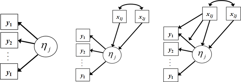
note: The scoring models were used to obtain factor score estimates of to be used in subsequent regression models. These are conceptual representations, the specifics of which are defined via equations in the text. In the left panel, no covariates were included in scoring; in the middle panel, the covariates were only related to the mean and variance of the latent factor; in the right panel, the covariates were related to the mean and variance of the latent factor and the item loading and intercept. The diagram shows two covariates for simplicity, but three were used in the simulations.
Unconditional.
In the unconditional scoring model, all three covariates were omitted from the analysis. Given that all of the item indicators were binary, this model is equivalent to an unconditional confirmatory factor analysis model with binary indicators or a two-parameter logistic IRT model (e.g., Takane & de Leeuw, 1987). This model is misspecified in that the covariates were present in the population measurement model but were omitted from the sample scoring model.
Impact-only.
In the impact-only scoring model, the three covariates were included in the measurement model, but the effects were limited to just the mean and variance of the latent variable (thus corresponding to Equations 1 and 2). This model is misspecified in that effects existed between the covariates and the item parameters in the population model but were omitted from the scoring model.
Impact-DIF.
In the impact-DIF scoring model, the model estimated in the sample precisely corresponded to that in the population generating model (thus corresponding to Equations 1 through 4). This is a properly specified model in that all covariate effects that existed in the population model were estimated in the sample scoring model.
Regression Models
Factor score estimates () were obtained from each of the three scoring models and were used as predictors in each of the three regression models described earlier (thus replacing with in Equations 6, 7 and 8). For each cell in the design (108 cells with 500 replications per cell), individual regression models were estimated using SAS PROC REG (Version 9.4, SAS Institute).
Criterion Measures: Relative Bias and Root Mean Squared Error
As with any comprehensive simulation study, a plethora of potential outcome measures were available. To optimally evaluate our research hypotheses we focused on bias (relative) and root mean squared error, or RMSE). We chose to focus on relative bias because no covariates are defined to have population values equal to zero and thus relative bias offers an interpretable and meaningful metric; we took values exceeding 10% to be potentially meaningful2. We also considered the RMSE because it balances bias and variability and offers a clear reflection of how far effect estimates tend to stray from their corresponding population values in any given replication. We graphically present a subset of findings in Figures 3 through 6 and a complete tabling of all results is available in the online appendix.
Figure 3. Relative bias for the second outcome (Z2) at a sample size of 500, one-third of items with large DIF, and small variance/large mean impact.

note: values of relative bias greater than +/−10% were taken as potentially meaningful.
Figure 6.

Root mean square error (RMSE) for the third outcome (Z3) at a sample size of 500, one-third of items with large DIF, and small variance/large mean impact.
Results
Regression Model: Outcome 1
The regression model for Outcome 1 consisted of a single, continuous outcome (z1j) regressed just on the factor score estimate; no covariates were included in this regression model.
Unconditional scoring model.
For the unconditional scoring model (where all covariates were omitted from factor score estimation) there were no design effects across any condition associated with observed relative bias in the estimated regression parameter exceeding 10%. Indeed, the vast majority of conditions were associated with relative bias falling below 5%. The unconditional model thus provided factor score estimates that well recovered the regression of the outcome on the score.
Impact-only scoring model.
In contrast to the unconditional model, the impact-only scoring model resulted in extensive bias in the predictor-criterion relation across multiple design conditions. The regression coefficient was routinely underestimated by 20% to 30%. The largest bias was found under conditions with the least amount of information and largest amount of omitted DIF (smaller sample size, smaller numbers of items, larger magnitude of DIF, and higher proportion of items with DIF).
Impact-DIF scoring models.
As was found for the unconditional scoring model, virtually no bias was found in the predictor-criterion relation for scores obtained under the impact-DIF scoring model. Indeed, there were no design effects across any condition associated with observed relative bias in the estimated regression parameter exceeding 10% and nearly all conditions reflected relative bias falling below 5%. This was expected given that the impact-DIF model was properly specified.
RMSE.
The RMSE values behaved as expected: in general, RMSE decreased with increasing numbers of items and increasing sample size, tended to be larger for coefficients associated with greater bias, and tended to increase slightly with the complexity of the scoring model. For example, for the unconditional scoring model with six items, medium impact, and large DIF influencing two-thirds of the items, RMSE was .15 at a sample size of 500, .10 at a sample size of 1000, and .07 for a sample size of 2000. In contrast, for the fully parameterized impact-DIF scoring model these same RMSE values were .18, .12, and .08, thus reflecting mostly comparable variability relative to the unconditional model. However, for the impact-only model, the RMSE values for these same conditions were .32, .28, and .26. This increase in the RMSE is directly attributable to the much higher bias observed for the impact-only scoring model relative to the other two scoring models.
Summary.
For the univariate regression model, the unconditional and impact-DIF scoring models resulted in little to no bias in the relation between the factor score and the outcome across all conditions and comparable RMSEs. In contrast, there was substantial bias in this same relation for the factor scores obtained from the impact-only model, particularly under conditions where there was smaller sample size, fewer items, and larger omitted DIF. This bias led to a sharp increase in the RMSE for impact-only model estimates relative to the other scoring models.
Regression Model: Outcome 2
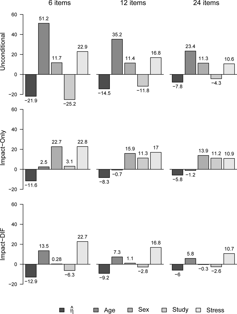
The regression model for Outcome 2 consisted of a single a continuous outcome (z2j) regressed on the factor score estimate and the main effects of three covariates (agej, sexj, and studyj). Because findings were consistent across nearly all design factors, Figure 3 presents relative bias and Figure 4 presents RMSE for a specific subset of exemplar conditions: six, 12, and 24 items assessed at a sample size of 500, small variance/large mean impact, and large DIF for one-third of the item set.3
Figure 4.

Root mean square error (RMSE) for the second outcome (Z2) at a sample size of 500, one-third of items with large DIF, and small variance/large mean impact.
Unconditional scoring model.
Modest bias was found in the regression of the outcome on the factor score estimate ranging from approximately –10% to –15%, but this was only found in the six-item condition. Bias was mitigated by decreasing magnitude of impact and increasing number of items such that minimal bias was found in all other 12- and 24-item conditions.
In contrast, extensive bias was found in the relations between all three covariates and the outcome, the magnitude and direction of which varied across covariates and design conditions. For example, the covariate age was associated with extensive positive bias ranging from approximately 20% to 50% across all conditions under large mean impact, and this bias was reduced at lower levels of impact. The covariate sex also showed positive bias, but to a lesser extent (ranging from approximately 10% to 30%); unlike the first covariate, bias increased as a function of decreasing mean impact. Finally, the covariate study showed bias ranging as high as nearly 25%, but this reflected underestimation of the regression effects whereas the first two covariates reflected overestimation of the regression effects. Bias for the third covariate was most severe with larger mean impact, and decreased in magnitude with decreasing magnitude of impact.
Impact-only scoring model.
Little bias was found in the recovery of the relation between the factor estimate and the outcome. Only four of 108 conditions reflected relative bias exceeding 10%, and the largest of these was 15% for the smallest sample size, fewest items, largest and most pervasive DIF, and smallest mean impact. All other estimates of bias were negligible.
However, as was found with the unconditional model, extensive bias was found across all conditions in the recovery of the relation between each of the three covariates and the outcome. Bias was negative for age but positive for sex and study. Bias ranged from approximately –20% up to nearly +50% and was generally more pronounced with less information (smaller sample size and fewer items) and more pervasive DIF effects (greater in magnitude and higher in proportion of affected items).
Impact-DIF scoring model.
No meaningful bias was observed in either the relation between the factor score estimate and the outcome nor between any covariate and the outcome.
RMSE.
As was found with the first model, the RMSE largely behaved as expected: decreasing with increasing sample size and number of items and becoming larger for those coefficients displaying greater bias. Of greatest interest was the finding that the RMSE was generally comparable for the coefficient associated with factor score estimate across the three scoring models when compared within the same design conditions. For example, Figure 4 reflects nearly equal RMSE values for the factor score coefficient for the unconditional, impact-only, and impact-DIF scoring models within each item set (these values are shown in the darkest shaded bar in the histogram). This is as expected given the associated coefficients reflected minimal bias. However, for the remaining coefficients that did display greater bias, the RMSE was generally smaller for the more complex scoring models (i.e., impact-only and impact-DIF models). Almost without exception, the impact-DIF scoring model showed the lowest RMSE.
Summary.
With a few minor exceptions, the relation between the factor score estimate and the outcome was unbiased for all three scoring models across all experimental design conditions (the exception being six items for the unconditional scoring model). However, extensive bias was found between the covariates and the outcome for the unconditional and impact-only scoring models, whereas no covariate bias was found with the impact-DIF scoring model. Thus, although the factor score estimate itself was associated with generally unbiased regression effects, the covariates were strongly biased for the unconditional and the impact-only scoring models. Finally, the RMSE decreased with increasing sample size and number items and decreasing bias; RMSE was lowest for the impact-DIF scoring model across nearly all conditions.
Regression Model: Outcome 3
The regression model for Outcome 3 differed from that for Outcome 2 given the inclusion of a covariate (stressj) that was correlated with the latent factor in the population but was not included in any of the three scoring models. This model was designed to mimic the common strategy used in practice in which covariates are included in a secondary analysis that were not used as part of the initial scoring stage of the analysis (e.g., Hussong et al., 2008, 2010, 2012). Because findings were generally consistent across all design factors, Figure 5 presents relative bias and Figure 6 present RMSE for the same subset of conditions as the prior model: six, 12, and 24 items at a sample size of 500, small variance/large mean impact, and large DIF for one-third of the items.
Figure 5. Relative bias for the third outcome (Z3) at a sample size of 500, one-third of items with large DIF, and small variance/large mean impact.
note: values of relative bias greater than +/−10% were taken as potentially meaningful.
Unconditional scoring model.
Unlike the first two regression models, the effects of the unconditional factor scores reflected substantial bias, in some instances approaching –25%. These levels of bias were primarily found across all three sample sizes for six and 12 items, but not for 24 items, and bias diminished with decreasing magnitude of mean impact. The effects of the three covariates that were also involved in the measurement model were biased in much the same way as was found in Regression Model 2; bias was positive for age and sex, and negative for study, the magnitude of which again varied in complex ways across design conditions.
However, extensive bias was found across nearly all experimental conditions in the regression of the outcome on the fourth covariate stressj. Recall that this fourth covariate played only a small role in the measurement model (via the correlation of the covariate with the disturbance of the latent factor) and the predictive effects were properly specified within the regression model. The pattern of bias is clearly related to one dominating influence: number of items. Bias was most evident with six items but decreased at 12 items and further still at 24 items. Values of relative bias approach 25% for six items at a sample size of 500, yet remained elevated at levels of 10% to 12% for 24 items at a sample size of 2000.
Impact-only scoring model.
Similar to the unconditional factor score, the impact-only score estimate showed evidence of negative bias in the prediction of the outcome, but this was primarily limited to the six item condition, and this diminished with increasing sample size. This is in contrast to Regression Model 2 in which no bias was observed in the regression of the outcome on the factor score estimate. Also similar to the unconditional factor score model, moderate to substantial bias was observed in the effects of all three covariates on the outcome, the magnitude of which varies over covariate and design condition.
The effect of the fourth covariate on the outcome was again substantially positively biased, but the bias was clearly mitigated by increasing number of items and modestly mitigated by decreasing levels of mean impact. Positive relative bias ranged as high as nearly 25%, and this was most pronounced under the six item condition. However, even at a sample size of 2000 with 24 items, relative bias still exceeded 10%.
Impact-DIF scoring model.
Modest bias was observed in the regression of the outcome on the impact-DIF factor score estimate of the same form as was found in the impact-only scoring model. Some under-estimation was observed for six items, but this diminished with increasing numbers of items and increasing sample size. Further, unlike Regression Model 2, there was evidence of positive bias associated with the covariate age, but only for the six item condition. Relative bias ranged up to 15%, but this rapidly diminished with increasing items, larger sample sizes, and decreasing levels of mean impact. The remaining two covariates showed no evidence of meaningful bias across any condition.
The regression of the outcome on the fourth covariate was substantially positively biased in much the same way as was found under the other two scoring models. Relative bias approached 25% at the smallest sample size and lowest number of items; this biased diminished with increasing numbers of items, increasing sample size, and decreasing mean impact. However, bias still remained above 10% even with 24 items and a sample size of 2000 for the large impact condition.
RMSE.
As with prior models, RMSE decreased with increasing sample size and number of items and tended to be larger for coefficients displaying greater bias. Further, for a given parameter within a given condition, the RMSE was generally smallest for the impact-DIF scoring model relative to the unconditional and impact-only scoring models, each of which tended to be comparable to the other. Consistent with the findings from Outcome 2, for Outcome 3 the RMSE for the coefficient associated with the factor score estimate was comparable across all three scoring models.
Summary.
Unlike the regression models for Outcomes 1 and 2, the factor score estimates for Outcome 3 showed moderate to substantial bias for all three scoring models in the presence of a covariate that was not included in the scoring model but was included in the regression model. This bias was most pronounced under conditions of less available information, namely smaller sample size and fewer items. This held even for the properly specified impact-DIF factor score estimates that in prior models showed no bias in any design condition. Further, the factor score estimate coefficient in Outcome 3 displayed much higher RMSEs than were observed for the same effect for Outcome 2, and this was primarily due to the greater bias associated with the effect estimate. Jointly, these are striking findings given the common practice of excluding a predictor from the scoring model but including that same predictor in subsequent analyses, the exact condition the fourth covariate was designed to mimic.
Additional Regression Model: Outcome 2 with the Inclusion of a Null Interaction
It is increasingly common to test higher-order interaction effects to examine conditional relations, particularly when striving to enhance replicability of findings (e.g., Anderson & Maxwell, 2016). This is particularly salient in many integrative data analysis applications in which interactions are defined among one or more covariates and study membership in order to account for differential covariate effects across contributing study (e.g., Curran et al. 2007, 2014; Hussong et al., 2008, 2010). To examine Type I error rates associated with a null interaction effect, we expanded the regression model for Outcome 2 defined in Equation (7) to include a null interaction between study membership (studyj) and the factor score estimate (). There are no measures of relative bias given that the population value is equal to zero (representing the null effect). We instead computed empirical rejection rates (taken at α =.05) as an estimate of Type I error. Given the null interaction, the empirical rejection rates should ideally approximate the nominal rate of 5%.
For the unconditional factor scores, the grand mean rejection rate (pooling over all cells of the design) was .19 with a cell mean range of .06 to .60. For the impact-only factor scores, the grand mean was .07 with a cell mean range of .04 to .14; and for the impact-DIF factor scores, the grand mean was .08 with a cell mean range of .04 to .15. There was thus slight elevation in the Type I error rates for the impact-only and impact-DIF scores with the highest rates occurring under conditions of larger sample size and larger number of items. However, the unconditional scores were associated with markedly elevated Type I error rates, with many design cells exceeding .30 and above. The greatest levels of inflation occurred under conditions of larger sample sizes and larger numbers of items, and this was modestly attenuated with higher levels of impact.
Discussion
There is no question that when a given experimental design and associated data allow, latent variables are best modeled directly within any empirical application (e.g., Bollen, 1989; 2002; Skrondal & Laake, 2001; Tucker, 1971). Despite this truism, there remain many contemporary applications in the social, behavioral, and health sciences in which the direct estimation of a latent factor is intractable and some type of factor score estimate is required. Somewhat ironically, the need for scale scores may actually be increasing with time given the substantial complications introduced in many advanced modeling methods that even further preclude the ability to model latent factors directly (e.g., mixture modeling, multilevel modeling, latent change score analysis, machine learning methodologies). Although much is known about factor score estimation in terms of true score recovery, much less is known about how these factor scores perform as most commonly used in subsequent analysis, particularly when used as predictors in the presence of covariates that were used in the scoring model itself. This was the focus of our work here.
We incorporated a comprehensive simulation design to empirically examine predictor-criterion recovery using three types of factor score estimates that were then used in one of three second-stage regression models. We examined the univariate and partial effects of the factor score estimate in the prediction of a continuous outcome as well as the partial effects of the covariates and that of a correlated predictor. Consistent with prior research, the parameterization of the optimal scoring model strongly depends on how the scores will be used in second-stage regression analysis and what effects are of primary substantive interest. We can distill our findings down to five lessons learned.
Lessons Learned
Lesson 1.
If the factor score estimate is to be used in a simple single-predictor regression that includes no other covariates, the covariates may either be entirely omitted from the scoring model or be fully parameterized in the scoring model; however, misspecification of the covariate effects in the scoring model leads to substantial bias in the second-stage regression model. Consistent with statistical theory and prior empirical results, factor score estimates obtained from a properly specified scoring model that included both impact and DIF resulted in unbiased regression coefficients with the lowest RMSE in the second-stage model. Somewhat unexpectedly, a similar lack of bias and comparable RMSE was found in the unconditional scoring model in which the covariates are omitted entirely. However, if the covariates are included in the scoring model but the effects are misspecified (e.g., inappropriately omitting DIF), substantial bias and increased RMSE was found in the second-stage regression model. A critical caveat to this conclusion is that rarely if ever would a bivariate correlation be the sole focus in practice thus limiting the utility of the unconditional scores. As such, more realistic models must be considered to fully understand the nature of these effects.
Lesson 2.
If the factor score estimate is used as a predictor in a second-stage regression that includes the same covariates used in the scoring model, then any of the three scoring models result in little to no bias in the partial regression coefficient between the outcome and the score estimate net the covariates. This finding was expected from theory for the fully parameterized impact-DIF model, but was unexpected for the misspecified impact-only model. More specifically, recall that the impact-only factor score estimates were strongly biased in the second-stage regressions when defined as a univariate predictor, yet little to no bias was found when this same effect was evaluated net the joint effects of the scoring covariates. There was a similar lack of bias in the partial effects of the unconditional factor score estimate. Interestingly, RMSE was mostly comparable within a set of experimental conditions across the three scoring methods. Taken together, this is somewhat heartening news in that unbiased regression coefficients were found regardless of scoring model, yet examination of the regression coefficients for the covariates themselves raises a substantial corollary to this conclusion.
Lesson 3.
If substantive interest is also placed on the effects of the covariates on the outcome in the second-stage regression model, then only the fully specified impact-DIF scoring models provides unbiased regression coefficients for both the factor score estimate and the covariate effects. Although Lesson 2 reflected that the partial effects of all three factor score estimates were largely unbiased net the effects of the scoring covariates, the reverse was unambiguously not true. Covariate effects net the influence of the factor score estimate were substantially biased across nearly all experimental conditions for both the unconditional and impact-only scoring models. Indeed, relative bias routinely fell in the 20% to 40% range, in some conditions overestimating and in other conditions underestimating the corresponding population effect. In contrast, little to no bias was observed for the fully specified impact-DIF scoring model. The RMSE for the coefficient estimates was as expected with greater RMSE associated with parameters characterized by greater bias, and lower RMSE with larger sample size and additional numbers of items. Further evidence of bias was reflected in that unconditional and impact-only score estimates resulted in markedly elevated Type I error rates in the estimation of spurious score-by-covariate interactions, an effect commonly estimated in practice. This is a truly intriguing finding: if the covariate effects are either omitted entirely or included by misspecified, the resulting factor score estimates carry information about this misspecification forward that in turn leads to bias in the covariates in the second-stage models. In the second-stage regression the covariates are serving to “absorb” the misspecification that occurred in the first-stage scoring model (Kaplan & Wenger, 1993).
Lesson 4.
If a second-stage model includes a predictor that is correlated with the latent factor but was not included in the scoring model, substantial bias will result in the estimated effect of the correlated predictor in the presence of the factor score estimate and the scoring covariates regardless of scoring model. Almost without exception, substantial bias and elevated RMSE was found across all experimental conditions in the partial regression coefficient between correlated predictor and the second-stage outcome for all three scoring models. This was expected from theory (see particularly Skrondal & Laake, 2001), yet this remains a deeply troubling result from the perspective of an applied researcher. It is a common strategy to first estimate a score for some theoretical construct (e.g., depression) and then use this as one of a set of exogenous covariates (e.g., stress, sex, age) in the prediction of an outcome (e.g., substance use). In this example, if stress is truly correlated with the latent factor of depression (which would be expected), and factor score estimates are obtained for depression in the absence of stress (which would commonly be done), then the prediction of substance use from stress net the effect of depression will be strongly biased in large and unpredictable ways. Even using the fully specified impact-DIF scoring model does not mitigate this bias because, although properly specified with respect to the three covariates, it is misspecified with respect to the correlated predictor. Much additional work is needed to determine how to best address this common situation.
Lesson 5.
All of the above effects tended to be mitigated by greater information, but greater information alone does not ameliorate bias. Consistent with both statistical theory and prior empirical findings, bias tended to be lower and coefficients estimated with lower RMSE under conditions of greater information (more items and larger sample sizes), smaller magnitude of impact effects, and smaller magnitude of DIF effects that influence a lower proportion of available items. Importantly, although key findings described above were less evident with greater numbers of items and larger sample sizes, substantial bias remained even under conditions with the most available information (24 items and 2000 cases). Thus greater information, although beneficial in a variety of ways, will not wholly eradicate the problems at hand.
Recommendations for Researchers
Our results uniquely contribute to a growing body of work that can help inform how substantive researchers can best obtain optimal factor score estimates for use in second-stage analysis. Our prior work demonstrated that impact-DIF scores were universally superior to unconditional and impact-only scores in terms of true score recovery (Curran et al., 2016). This is what Tucker (1971) considers “internal” characteristics. Our current work offers particularly salient insights into the use of covariate-informed scores that capture impact and DIF effects in second-stage analysis, a condition under which score are used in practice. This is what Tucker (1971) considers “external” characteristics. These external characteristics are of greatest importance to the applied researcher.
Based on the results presented here, we offer four primary recommendations for how to optimize the external characteristics of factor scores as applied in second-stage analyses. First, it is important for researchers to identify relevant covariates that influence the expression of the latent factor in terms of impact and DIF and, once identified, these covariates must be included in the scoring model when obtaining factor score estimates. Which covariates to include and which to exclude are primarily theoretically motivated and justified, although empirical results can help guide selection. Second, a principled approach should be taken when building the impact-DIF scoring model, although precisely what approach is best remains unclear. We have previously offered recommendations that describe a sequential process using likelihood ratio tests (Curran et al., 2014), although this is tedious and can be influenced by the idiosyncratic characteristics of the given sample. Exciting ongoing work is moving toward an automation of this model building process (e.g., Gottfredson et al., 2018). Third, all covariates included in the scoring model should also be included in the second-stage regression model to obtain accurate estimates of both factor score and covariate effects on the outcome measure. Fourth, it is currently unclear how to best mitigate bias introduced by predictors that are correlated with the latent factor but are not included in the scoring model. Our results suggest that all predictors that are correlated with the latent factor should be included in the scoring model, but there are clearly limits to the number of covariates that can be stably included and future research is strongly needed to better understand this important issue.
Limitations and Directions for Future Research.
Our results contribute to the existing literature on scoring in several important ways. Most notably, to our knowledge this is the first comprehensive examination of the role of exogenous covariates on the scoring of the latent factor under conditions of both impact and DIF. Both Skrondal and Laake (2001) and Lu and Thomas (2008) presented important findings about factor scoring for continuous and discrete items, respectively, but neither considered the additional influences of impact and DIF. The inclusion of impact and DIF effects is an important topic to consider given the recent development of novel methods for estimating these effects in ways not previously possible (Bauer, 2017; Bauer & Hussong, 2009) and in the ubiquity of impact and DIF in many research settings (particularly in applications of integrative data analysis; e.g., Hussong et al., 2008, 2010, 2012). Our study was designed to rigorously study the role of impact and DIF in scoring and was characterized by a number of significant strengths including the use of three different scoring models and three second-stage regression models spanning a large range of experimental conditions commonly encountered in practice. However, there are several potential limitations of our design.
First, we jointly placed our focus on measures of relative bias and RMSE as these are of greatest importance in applied research settings. Additional insights could be gained by consideration of standard errors and confidence interval estimation as well as examination of other model-specific outcomes (e.g., coefficient of determination, mean squared error). Second, we did not consider the behavior of the most widely used method of scoring, the sum score. Our rationale was that this is a psychometrically inferior measurement model and our prior results empirically showed it performed worst of all other factor score estimation methods. Although the field would do well to move towards more psychometrically rigorous models (such as those studied here), it would be helpful to better understand how these complex impact and DIF effects are manifested for the sum score. Third, we only consider the latent factor as an exogenous variable in the second-stage regression models. Both Skrondal and Laake (2001) and Lu and Thomas (2008) demonstrate that bias differs as a function of scoring method and exogenous-endogenous distinction in the fitted models. Our results could be expanded to address accuracy of recovery when the latent factor is itself endogenous; it would be particularly interesting to consider conditions in which the factor is a mediator and thus simultaneous serves as both a predictor and criterion.
Finally, arguably the most important direction for future research is on the study of how to best include exogenous measures that are correlated with the latent factor but are not related to impact or DIF. Not only was this correlated predictor substantially biased across all conditions under study, but this situation is common across nearly all applied research settings. This presents a striking potential problem in nearly any research application in which there may exist a large number of covariates that are of interest in the second-stage model yet are not included in the first-stage scoring model. Developing a better understand of this issue and establishing effective analytic strategies for mitigating the resulting bias is a research priority.
Acknowledgments
This research was supported by R01DA034636 (Daniel Bauer, Principal Investigator).
Footnotes
We later expanded this model to include a null interaction between the factor score estimate and the first covariate to evaluate Type I error rates; more will be said about this later.
We also fit a series of general linear models (GLMs) to both raw bias and RMSE (e.g., Skrondal, 2000). We do not present these results here because the GLMs do not shed any additional light on the findings beyond our discussion of relative bias and RMSE. Complete GLM results are presented in the online appendix.
Complete results are presented in the online appendix.
References
- Anderson SF, & Maxwell SE (2016). There’s more than one way to conduct a replication study: Beyond statistical significance. Psychological Methods, 21, 1–12. [DOI] [PubMed] [Google Scholar]
- Anderson TW, & Rubin H (1956). Statistical inference in factor analysis. In Proceedings of the third Berkeley symposium on mathematical statistics and probability (Vol. 5, pp. 111–150). [Google Scholar]
- Bartlett MS (1937). The statistical conception of mental factors. British Journal of Psychology. General Section, 28, 97–104. [Google Scholar]
- Bauer DJ (2017). A more general model for testing measurement invariance and differential item functioning. Psychological Methods, 22, 507–526. [DOI] [PMC free article] [PubMed] [Google Scholar]
- Bartholomew DJ, & Knott M (1999). Latent variable models and factor analysis (2nd). London: Arnold. [Google Scholar]
- Bauer DJ, & Hussong AM (2009). Psychometric approaches for developing commensurate measures across independent studies: traditional and new models. Psychological methods, 14(2), 101. [DOI] [PMC free article] [PubMed] [Google Scholar]
- Bentler PM, & Weeks DG (1980). Linear structural equations with latent variables. Psychometrika, 45, 289–308. [Google Scholar]
- Bock RD, & Aitkin M (1981). Marginal maximum likelihood estimation of item parameters: Application of an EM algorithm. Psychometrika, 46, 443–459. [Google Scholar]
- Bollen KA (1989). Structural Equations with Latent Variables. New York: John Wiley & Sons. [Google Scholar]
- Bollen KA (2002). Latent variables in psychology and the social sciences. Annual Review of Psychology, 53, 605–634. [DOI] [PubMed] [Google Scholar]
- Curran PJ (2009). The seemingly quixotic pursuit of a cumulative psychological science: introduction to the special issue. Psychological Methods, 14, 77–80. [DOI] [PMC free article] [PubMed] [Google Scholar]
- Curran PJ, Cole V, Bauer DJ, Hussong AM, & Gottfredson N (2016). Improving factor score estimation through the use of observed background characteristics. Structural Equation Modeling: A Multidisciplinary Journal, 23, 827–844. [DOI] [PMC free article] [PubMed] [Google Scholar]
- Curran PJ, & Hussong AM (2009). Integrative data analysis: the simultaneous analysis of multiple data sets. Psychological Methods, 14(2), 81–100. [DOI] [PMC free article] [PubMed] [Google Scholar]
- Curran PJ, McGinley JS, Bauer DJ, Hussong AM, Burns A, Chassin L, Sher K, & Zucker R (2014). A moderated nonlinear factor model for the development of commensurate measures in integrative data analysis. Multivariate behavioral research, 49(3), 214–231. [DOI] [PMC free article] [PubMed] [Google Scholar]
- Edelen MO, Stucky BD, & Chandra A (2015). Quantifying ‘problematic’ DIF within an IRT framework: application to a cancer stigma index. Quality of Life Research, 24(1), 95–103. [DOI] [PubMed] [Google Scholar]
- Gottfredson NC, Cole VT, Giordano ML, Bauer DJ, Hussong AM, & Ennett ST (2018). Simplifying the implementation of modern scale scoring methods with an automated R package: Automated moderated nonlinear factor analysis (aMNLFA). Manuscript submitted for publication. [DOI] [PMC free article] [PubMed] [Google Scholar]
- Greenbaum PE, Wang W, Henderson CE, Kan L, Hall K, Dakof GA, & Liddle HA (2015). Gender and ethnicity as moderators: Integrative data analysis of multidimensional family therapy randomized clinical trials. Journal of Family Psychology, 29, 919–930. [DOI] [PMC free article] [PubMed] [Google Scholar]
- Hansen M, Cai L, Stucky BD, Tucker JS, Shadel WG, & Edelen MO (2014). Methodology for developing and evaluating the PROMIS® smoking item banks. Nicotine & Tobacco Research, 16 (Suppl. 3), S175–S189. doi: 10.1093/ntr/ntt123 [DOI] [PMC free article] [PubMed] [Google Scholar]
- Hoshino T, & Bentler PM (2013). Bias in factor score regression and a simple solution In De Leon AR, and Chough KC (Eds.), Analysis of Mixed Data: Methods & Applications (pp. 43–61). Boca Raton, FL: CRC Press, Taylor & Francis Group. [Google Scholar]
- Hussong AM, Flora DB, Curran PJ, Chassin LA, & Zucker RA (2008). Defining risk heterogeneity for internalizing symptoms among children of alcoholic parents. Development and psychopathology, 20(01), 165–193. [DOI] [PMC free article] [PubMed] [Google Scholar]
- Hussong AM, Huang W, Curran PJ, Chassin L, & Zucker RA (2010). Parent alcoholism impacts the severity and timing of children’s externalizing symptoms. Journal of Abnormal Child Psychology, 38, 367–380. [DOI] [PMC free article] [PubMed] [Google Scholar]
- Hussong AM, Huang W, Serrano D, Curran PJ, & Chassin L (2012). Testing whether and when parent alcoholism uniquely affects various forms of adolescent substance use. Journal of Abnormal Child Psychology, 40, 1265–1276. [DOI] [PMC free article] [PubMed] [Google Scholar]
- Hussong AM, Wirth RJ, Edwards MC, Curran PJ, Zucker RA, & Chassin LA (2007). Externalizing symptoms among children of alcoholic parents: Entry points for an antisocial pathway to alcoholism. Journal of Abnormal Psychology, 116, 529–542. [DOI] [PMC free article] [PubMed] [Google Scholar]
- Jöreskog KG (1973), A general method for estimating a linear structural equation system. In Structural Equation Models in the Social Sciences, Goldberger AS and Duncan 0D, Eds. New York: Seminar Press, 85–112. [Google Scholar]
- Kaplan D, & Wenger RN (1993). Asymptomatic independence and separability in covariance structure models: Implications for specification error, power, and model modification. Multivariate Behavioral Research, 28, 467–482. [DOI] [PubMed] [Google Scholar]
- Lu IR, & Thomas DR (2008). Avoiding and correcting bias in score-based latent variable regression with discrete manifest items. Structural Equation Modeling, 15, 462–490. [Google Scholar]
- McDonald RP (1981). The dimensionality of tests and items. British Journal of Mathematical and Statistical Psychology, 34, 100–117. [Google Scholar]
- McDonald RP (2001). Measuring latent quantities. Psychometrika, 76, 511–536. [DOI] [PubMed] [Google Scholar]
- Millsap RE, & Kwok OM (2004). Evaluating the impact of partial factorial invariance on selection in two populations. Psychological Methods, 9, 93–115. [DOI] [PubMed] [Google Scholar]
- Mislevy R, Johnson E, & Muraki E (1992). Scaling procedures in NAEP. Journal of Educational Statistics, 17, 131–154. [Google Scholar]
- Raykov T (2012). Propensity score analysis with fallible covariates: A note on a latent variable modeling approach. Educational and Psychological Measurement, 72, 715–733. [Google Scholar]
- Rose JS, Dierker LC, Hedeker D, & Mermelstein R (2013). An integrated data analysis approach to investigating measurement equivalence of DSM nicotine dependence symptoms. Drug and alcohol dependence, 129, 25–32. [DOI] [PMC free article] [PubMed] [Google Scholar]
- SAS Institute Inc. (2013). Base SAS® 9.4 Procedures Guide: Statistical Procedures, Second Edition Cary, NC: SAS Institute Inc. [Google Scholar]
- Skrondal A (2000). Design and analysis of Monte Carlo experiments: Attacking the conventional wisdom. Multivariate Behavioral Research, 35, 137–167. [DOI] [PubMed] [Google Scholar]
- Skrondal A, & Laake P (2001). Regression among factor scores. Psychometrika, 66, 563–575. [Google Scholar]
- Southworth J, Mancini L, Madhusudhan N, Mollière P, Ciceri S, & Henning T (2017). Detection of the Atmosphere of the 1.6 M⊕ Exoplanet GJ 1132 b. The Astronomical Journal, 153, 191. [Google Scholar]
- Spearman C (1904). The proof and measurement of association between two things. The American journal of psychology, 15(1), 72–101. [PubMed] [Google Scholar]
- Steiger JH, & Schönemann PH (1978). A history of factor indeterminacy In Shye S (Ed.) Theory Construction and Data Analysis in the Behavioral Sciences, San Francisco, Jossey-Bass, pp. 136–178. [Google Scholar]
- Takane Y, & de Leeuw J (1987). On the relationship between item response theory and factor analysis of discretized variables. Psychometrika, 52, 393–408. [Google Scholar]
- Thomson GH (1936). Some points of mathematical technique in the factorial analysis of ability. Journal of Educational Psychology, 27, 37–54. [Google Scholar]
- Thurstone LL (1935). The vectors of the mind. Chicago: University of Chicago Press. [Google Scholar]
- Tucker LR (1971). Relations of factor score estimates to their use. Psychometrika, 36(4), 427–436. [Google Scholar]
- Vartanian TP (2010). Secondary Data Analysis. Oxford University Press. [Google Scholar]