iSEE: Interface structure, evolution, and energy‐based machine learning predictor of binding affinity changes upon mutations

Abstract

Quantitative evaluation of binding affinity changes upon mutations is crucial for protein engineering and drug design. Machine learning‐based methods are gaining increasing momentum in this field. Due to the limited number of experimental data, using a small number of sensitive predictive features is vital to the generalization and robustness of such machine learning methods. Here we introduce a fast and reliable predictor of binding affinity changes upon single point mutation, based on a random forest approach. Our method, iSEE, uses a limited number of interface Structure, Evolution, and Energy‐based features for the prediction. iSEE achieves, using only 31 features, a high prediction performance with a Pearson correlation coefficient (PCC) of 0.80 and a root mean square error of 1.41 kcal/mol on a diverse training dataset consisting of 1102 mutations in 57 protein‐protein complexes. It competes with existing state‐of‐the‐art methods on two blind test datasets. Predictions for a new dataset of 487 mutations in 56 protein complexes from the recently published SKEMPI 2.0 database reveals that none of the current methods perform well (PCC < 0.42), although their combination does improve the predictions. Feature analysis for iSEE underlines the significance of evolutionary conservations for quantitative prediction of mutation effects. As an application example, we perform a full mutation scanning of the interface residues in the MDM2–p53 complex.

1. INTRODUCTION

The affinity between proteins and their binding partners is a fundamental property that governs their function in cells. Mutations in proteins can induce changes in the binding affinity for their interaction partners, altering their functioning by perturbing their communication network. Missense mutations are often linked to various human diseases,1 such as cancer. Quantitative characterization of binding affinity changes can therefore shed light on the relation between coding variations and disease phenotypes, and guide the design of effective therapeutics for genetic disorders. It can also be particularly useful for engineering protein–protein interactions with modulated binding affinity.

Various experimental methods can be used to quantitatively measure binding affinities,2, 3 each with their own limitations and precision. Although they provide valuable information, experimental methods can be labor‐intensive and time‐consuming, and, as a consequence, lag behind the rapid advances of sequencing technologies, which are generating a huge amount of data on disease‐causing mutations. This calls for the development of reliable and fast computational methods for estimating the mutation effects on binding affinity (ie, the binding free energy change between a wild type and mutant complex, ΔΔG).

Computational methods for ΔΔG prediction can be largely grouped into three main strategies: (1) Rigorous methods, such as thermodynamic integration and free energy perturbation,4, 5 (2) empirical energy‐based methods, based for example on classical mechanics or statistical potentials6, 7, 8, 9, 10 (typically in linear forms), and (3) machine learning‐based methods which can exploit a large variety of energetics and non‐energetics (eg, geometric, evolutionary) features.11, 12, 13 The rigorous methods can be accurate but they are computationally highly demanding. Their application is, therefore, limited to mainly low‐throughput and small system ΔΔG calculations. The empirical energy‐based methods are much faster and more broadly applied. They usually take a form of linear functions, often with only energy‐based terms, and fail to exploit evolution information, which can limit their ability to capture mutation effects on binding affinity. Insufficient conformational sampling, especially for mutations in flexible regions, can limit the accuracy of energy‐based methods. In contrast, machine learning‐based methods are potentially less sensitive to this since they can model mutation effects using not only potentials or energies but also other relevant features, such as, sequence, structure, and evolution. Machine learning approaches typically aim to model the intrinsic relationship between features of a mutation site and the response variable (eg, the binding affinity change) by training statistical models from mutation datasets with experimentally determined ΔΔG. Due to the data‐driven essence of machine learning, the availability of a large amount of reliable experimental data and the construction of features that can reflect structural and physico‐chemical changes caused by mutations are crucial factors in the success of this type of methods. It is therefore not surprising that the publication of the SKEMPI database14 (version 1.1, which was in the past 6 years the largest mutation ΔΔG dataset for protein–protein complexes containing 3047 mutations in 85 complexes) quickly promoted the emergence of several machine learning‐based ΔΔG predictors.11, 12, 13 However, the SKEMPI 1.1 dataset is still rather limited in size and one has to be careful not to use too many features to train a model to avoid overfitting problems. It is therefore important to design fast and reliable ΔΔG predictors that exploit only a limited number of sensitive and relevant features. Very recently, an update of SKEMPI was published, version 2.0,15 which provides a much extensive dataset and gives us the opportunity to test various predictors on data none of them has previously seen.

Residue conservation plays a central role in determining the binding affinity. It has been verified that the binding energy is not evenly distributed among the interfacial residues. Instead, some residues (hot‐spots) contribute most to the binding affinity.16, 17, 18 Such residues are often highly conserved. Interface conversation has been used in several of the best performing ΔΔG predictors.13, 19 However, since the conservation measure they used is structure‐based, relying on the availability of structural homologs,13, 19 the application and prediction of these ΔΔG predictors are largely limited by the availability and the number of such homologs. By contrast, conservation from Position Specific Scoring Matrix (PSSM) is sequence‐based and thus better applicable. The PSSM value is a log likelihood ratio between the observed probability of one type of amino acid appearing in a specific position in the multiple sequence alignment (MSA) and the expected probability of that amino acid type appearing in a random sequence.20 Thus, each position of a protein can be represented as a 20 by 1 PSSM profile (or vector), which captures the conservation property of each amino acid type at a specific position.

Here we present a machine learning‐based method named iSEE (interface Structure, Evolution and Energy‐based ΔΔG predictor), which combines HADDOCK21 structure and energy terms of wildtype and mutant complexes as well as PSSM conservation profiles before and after mutations (Figure 1). HADDOCK21 is our in‐house docking program, which has been consistently ranking among the top predictors and scorers in CAPRI, a community‐wide experiment for the prediction of biomolecular interactions.22 Its simple but sensible scoring function has contributed much to its success.23 It includes intermolecular van der Waals (Evdw) and Coulomb electrostatics (Eelec) energies, an empirical desolvation energy term (Edesolv)24 and buried surface area (BSA), which is only used in intermediate scoring steps and not in the final scoring function. iSEE is based on a random forest model25, 26 for ΔΔG prediction, trained on a subset of 1102 single point mutations in 57 complexes from SKEMPI 1.1. It uses a small number of features to lower the overfitting risk and competes with both empirical potentials‐ and machine learning‐based state‐of‐the‐art methods on an existing independent test dataset (the Benedix et al dataset8) and a large test dataset from the recently released SKEMPI 2.0 database. The recent release of SKEMPI 2.0 allows us for the first time to test various ΔΔG predictors on a large new blind dataset with about 500 mutations. Analysis of the importance of the features used in iSEE highlights the significance of evolutionary information in predicting the effect of mutations on the binding affinity of protein complexes. Using iSEE we performed a full computational mutation scanning of the interface of the MDM2–p53 complex and identified three important residues, two of which have been validated as hot‐spot experimentally.

Figure 1.

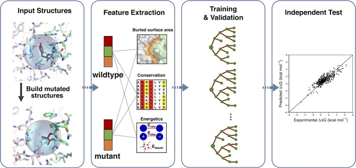
The workflow of iSEE predictor. Only the 3D structure of wildtype complex and the mutation information are necessary input for iSEE. We first model the mutated structure using HADDOCK (the water refinement web service). Then we extract features related to the evolutionary conservation and to changes in structure and energetics caused by the mutation. A random forest algorithm is then optimized and cross validated on a training dataset, resulting in our final ΔΔG predictor iSEE. Finally, iSEE is evaluated on two blind test datasets and compared with other current leading ΔΔG predictors

2. METHODS

2.1. Training and test datasets

Four datasets of experimental ΔΔG with available crystal structures of protein complexes were used in this study. Only single point mutations in the interface of the protein–protein complexes were considered, and only for dimeric complexes for ease of computations, but our prediction scheme can be easily extended to multimers. The interface residues were defined following Levy's method27 as those located in the core, rim, and support regions.

The training dataset was extracted from the DACUM database (https://github.com/haddocking/DACUM),28 our ΔΔG database derived from the SKEMPI 1.1 database.14 DACUM contains 1872 single point mutations in 81 protein complexes. After applying the above‐mentioned filter criteria, 1102 single point mutations in 57 protein complexes were selected.

We compiled two independent datasets, not used for training, to evaluate, and compare our predictor with state‐of‐the‐art ΔΔG predictors.

We selected a subset from the Benedix et al NM dataset8 for which predictions of various ΔΔG predictors have already been reported.7, 9 The original NM dataset has both single point and multiple point mutations in protein dimer or multimer complexes. We applied the same filtering criteria as above. Moreover, to avoid any overlap between the training dataset and the test dataset, mutations existing in the training dataset were filtered out from the original NM dataset. This procedure resulted in 19 mutations in one complex (PDB ID: 1IAR). For this heterodimer complex, only ΔΔG values for mutations on chain A were contained in our training dataset, while all ΔΔG data in the NM dataset are for mutations on chain B. Thus, the NM dataset is distinct from our training dataset at the level of mutation position. In the remaining of our article, we will refer to those data as “the NM dataset.”

Also, we selected new data from the recently released SKEMPI 2.0 database. After applying the above‐mentioned filter criteria, 487 mutations in 56 protein complexes were selected. We will refer to this dataset as “the S487 dataset” in the remaining article.

Finally, we used the MDM2–p53 complex for case study, which does not exist in SKEMPI. We obtained experimental ΔΔG values in our laboratory (van Rossum et al, manuscript in preparation) for 16 and 17 single point mutations at the interface of MDM2 and p53, respectively (PDB ID: 1YCR). Seven mutations that reach the experimental detection limitation have experimental ΔΔG of larger than 2 kcal/mol. The list of these mutations can be found in Supporting Information Table S8.

2.2. Predictive features

We compiled a list of 31 features (Supporting Information Table S4) including intermolecular energy terms and buried surface area (BSA) from HADDOCK21 and conservation values from PSSM.

To obtain the structural and energetic features, both wild type and mutant structures were refined using the protocol implemented in the refinement interface of the HADDOCK server.29 The mutations were introduced by simply changing the identity of the residue in the coordinate file and letting HADDOCK rebuild the missing side‐chain atoms and refine the interface in explicit solvent using the TIP3P water model and the Optimized Potentials for Liquid Simulations (OPLS) force field30 with an 8.5 Å cutoff for the non‐bonded interactions. The HADDOCK terms for wildtype or mutant complex were extracted from the top ranked HADDOCK model. The HADDOCK‐derived features are:

• Evdw, the intermolecular van der Waals energy described by a 12‐6 Lennard‐Jones potential.

• Eelec, the intermolecular electrostatic energy described by a Coulomb potential.

• Edesolv, an empirical desolvation energy term.24

• BSA, the buried surface area calculated by taking the difference between the sum of the solvent accessible surface area (SASA) for each individual protein and the SASA of the protein complex using 1.4 Å water probe radius.

The four HADDOCK terms of wildtype complex and the differences of the HADDOCK terms between mutant and wildtype complexes were used as HADDOCK‐based predictive features, which are named as Evdw_wt, Eelec_wt, Edesolv_wt, BSA_wt, Evdw_diff, Eelec_diff, Edesolv_diff, and BSA_diff.

The PSSM was calculated through PSI‐BLAST of BLAST 2.3.031 using a local version of the software and databases with the following parameters: BLOSUM62 was used as scoring matrix by default, and PAM30 was used when BLOSUM62 failed for short sequences; the number of iterations was 3 and the e‐value threshold was set to 0.0001; the BLAST database was the nr database (non‐redundant BLAST curated protein sequence database, version on 22nd August 2016). Default values were used for all the other parameters. For each mutation position of a query protein, four types of conservation features were extracted from the PSSM file:

• the PSSM profile for this position, which is a 20 by 1 vector (PSSM_AA).

• the information content for this position (PSSM_IC).

• the individual PSSM value for the wildtype residue at this position (PSSM_wt).

• the difference between the individual PSSM values for mutant residue and wildtype residue at this position (PSSM_diff).

2.3. Training procedures and evaluation metrics

We used the random forest algorithm26 from the R Caret package32 to train our ΔΔG predictor. We optimized the parameters of random forest over 10 times 10‐fold cross‐validations on the training dataset: the number of trees to grow, defined by the “ntree” parameter, was varied from 10 to 100 in steps of 10, and the number of variables randomly sampled as candidates at each split, defined the “mtry” parameter, was sampled from 1 to 20. The prediction performance was evaluated by root mean square error (RMSE) and Pearson's correlation coefficient (PCC).

2.4. Comparison with other ΔΔG predictors

The performance of the iSEE ΔΔG predictor was compared with several state‐of‐the‐art ΔΔG predictors on the independent NM and SKEMPI 2.0 S487 test datasets. For the NM dataset, the predicted ΔΔG values of pred1,9 pred2,9 CC/PBSA,8 BeAtMuSiC,10 and FoldX6 were directly extracted from Li et al.9 and those of ZeMu from Dourado's article.7 Predictions of mCSM11 and BindProfX19 for the test datasets were directly obtained from their respective webservers. The default parameters of BindProfX were used except the “Score to use” which was set to “interface profile and physics potential” (the authors reported it to work best for single point mutations19). A local version of FoldX (4.0) was used for the S487 dataset.

2.5. Classification of mutations

Mutations were classified based on three scenarios: the location of the mutation, the type of mutated amino acid and the change in the size of the amino acid side‐chain.

Based on the type of secondary structure a mutation is located, it was classified as a loop or non‐loop mutation. We used DSSP33, 34 (v2.0.4) for secondary structure assignment. DSSP code S, B, and blank were considered as loop, otherwise non‐loop.

Based on the type of mutated amino acid, a mutation was called “toALA” mutation when a residue was mutated to alanine, otherwise “toNonALA” mutation.

The change of amino acid size was defined as the difference of volumes (ΔV) between mutant and wildtype amino acids. The volumes of the 20 amino acids were taken from literature.35 A mutation was classified as “neutral” if |ΔV| ≤ 10 ų, as small to large (“toLarge”) if ΔV > 10 ų, and as large to small (“toSmall”) if ΔV < −10 ų.

2.6. Feature importance analysis

We used the algorithm from the R package randomForest26 to evaluate feature importance. The feature importance is measured by the decrease of mean squared error when splitting on a feature, averaged over all trees. The importance measure of a group of features was calculated by taking the sum of weighted importance of each feature in that group with the weight for each feature defined as the number of times the feature was chosen as split variable over all trees divided by the total of all group member features. The PSSM profile scores for the 20 amino acids were treated as a group (PSSM_AA). The best model trained on the entire training dataset with parameters ntree = 80 and mtry = 7 was used to analyze the feature importance.

2.7. Data and model availability

All PDB files including the HADDOCK‐refined models, and PSSM files used in this work are available from the SBGrid Data repository36 (doi:10.15785/SBGRID/520). The iSEE predictor and features used for training and test are freely available on GitHub from https://github.com/haddocking/iSee.

3. RESULTS

3.1. Training and validation of iSEE on a large diverse single point mutation dataset

We trained iSEE on a relatively large and diverse dataset consisting of experimental ΔΔG values for 1102 single point mutations in the interface of 57 dimer complexes. Among those, 656 mutations are in loops, 767 are non‐ALA mutations, 376 correspond to small to large substitutions, and 590 from large to small size (Supporting Information Table S5). For each mutation, we extracted 31 energetics and conservation features (see Methods). A random forest (RF) model was trained and evaluated using 10‐fold cross‐validation (CV). The data are randomly divided into 10 parts, 9 of which are used for training and the left‐out one for evaluating the performance of the trained RF model. This process was repeated 10 times to reduce the randomness of the data partition. From this training, a RF model with 80 trees and 7 randomly selected variables for each node achieved the best average root mean square error (RMSE) value (Figure S1 in Supporting Information). The resulting best performing ΔΔG predictor, called iSEE, was compared with state‐of‐the‐art ΔΔG predictors (see below).

iSEE's prediction performance shows an average RMSE of 1.41 ± 0.14 kcal/mol and a Pearson's correlation coefficient (PCC) of 0.80 ± 0.06 over the cross‐validated sets (Figure 2A). The predictor performs as well for ALA and non‐ALA mutations, mutations inside and outside loops, and mutations corresponding to different changes in side‐chain sizes (Figure 2B,D). This indicates that our approach is not very sensitive to possible conformational changes coming from loop flexibility and is robust for different types of mutations. We further evaluated the applicability of iSEE to different types of protein complexes. Our results show that iSEE has a strong generalizability for predicting ΔΔG trends for mutations within complexes (Supporting Information Figures S2 and S3).

Figure 2.

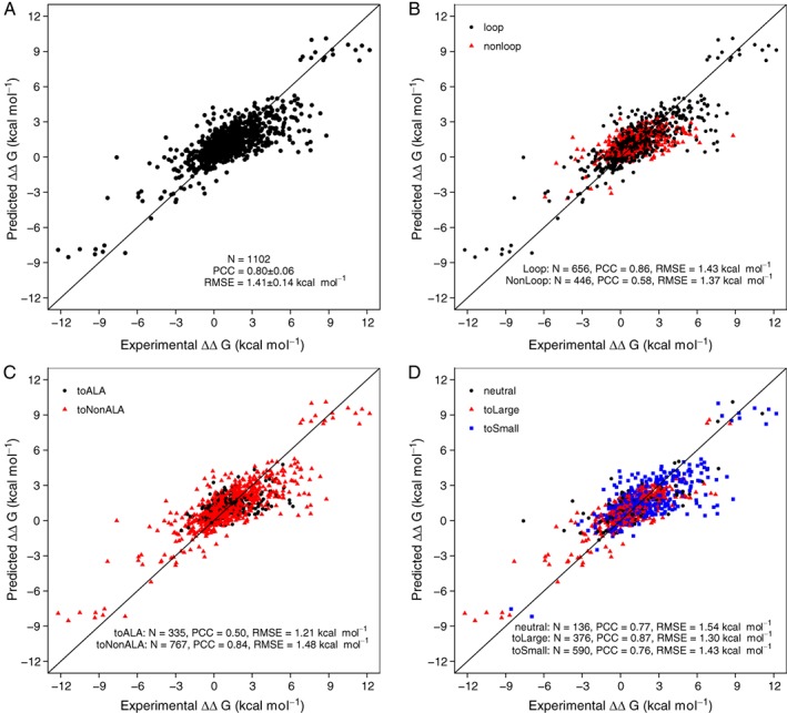
Correlations between predicted and experimental ΔΔG values for the training dataset consisting of 1102 single point mutations from the SKEMPI14/DACUM28 database. Ten times 10‐fold cross‐validation (CV) was applied during training, and the average of the CV predicted ΔΔG values are shown here for all mutations (A) and mutations classified as loop or non‐loop (B), type of mutated amino acid (C), and change in amino acid size (D). The diagonal indicates an ideal prediction. PCC is the Pearson's correlation coefficient and RMSE represents root mean squared error

3.2. iSEE competes with state‐of‐the‐art ΔΔG predictors

We evaluated the performance of our iSEE ΔΔG predictor on the blind Benedix et al dataset8 (see Methods) and compared it to several other state‐of‐the‐art ΔΔG predictors based on empirical potentials or machine learning methods, which have been tested by Li et al9 on the same data set. We only selected data from the NM data set for mutations that were not represented in the training data, which left 19 single point mutations for one complex (heterodimer, PDB ID: 1IAR. Supporting Information Table S6).

iSEE was compared with the following predictors:

• FoldX, which models free energy as a linear combination of multiple energy terms with weights optimized on a set of experimental ΔΔG values.6

• ZeMu, which can model conformational changes upon mutation using molecular dynamics simulations but relies on FoldX to predict ΔΔG.7

• CC/PBSA,8 pred1,9 and pred2,9 which generate an ensemble of structures and apply a Molecular Mechanics—Poisson–Boltzmann Surface Area (MM‐PBSA) approach to calculate the binding free energy.

• BeAtMuSiC, which is based on a linear combination of coarse grained statistical potentials.10

• mCSM,11 a machine learning based approach, using distance‐specific atom‐contacts (calculated from the wild‐type structures only) and pharmacophore changes of the mutation site as features of Gaussian processes to predict ΔΔG.

• BindProfX,19 which is mainly based on evolutionary interface profile constructed from structural homologs, and combines the interface profile score with FoldX through a simple linear function to predict ΔΔG.

iSEE compares favorably with the eight other predictors considered here over the independent NM test set with a RMSE of 1.37 kcal/mol and a PCC of 0.73 (Figure 3), belonging to the top four predictors with PCCs over 0.70: BindProfX (0.81), iSEE (0.73), FoldX (0.72), and ZeMu (0.70). The ΔΔG predictions of the top four predictors are statistically significant with p values lower than 0.001, while other predictors have larger p values ranging from 0.006 to 0.523. Note that since CC/PBSA did use the NM data for training,8 its performance might be over‐estimated.

Figure 3.

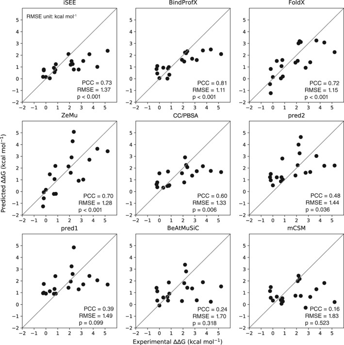
Predicted versus experimental ΔΔG for various ΔΔG predictors tested on a subset of the Benedix et al dataset8 consisting of 19 mutations for one complex, non‐overlapping with our training set. This subset was not used in any of the predictors, except for CC/PBSA. PCC is the Pearson's correlation coefficient, P is two tailed P value of PCC, and RMSE represents root mean squared error

3.3. There is still plenty of room to further improve ΔΔG predictors

We benchmarked iSEE and three other ΔΔG predictors (FoldX, mCSM, and BindProfX) on a much larger blind test dataset (the S487 dataset) constructed from the recently released SKEMPI 2.0 update. This dataset contains 487 mutations in 56 protein complexes that have not been seen by any predictor tested here (Supporting Information Table S7). None of the four ΔΔG predictors performs well on this large blind test set (Figure 4). BindProfX performs best with an RMSE of 1.20 kcal/mol and PCC of 0.41 while iSEE achieves an RMSE of 1.32 kcal/mol and PCC of 0.25.

Figure 4.

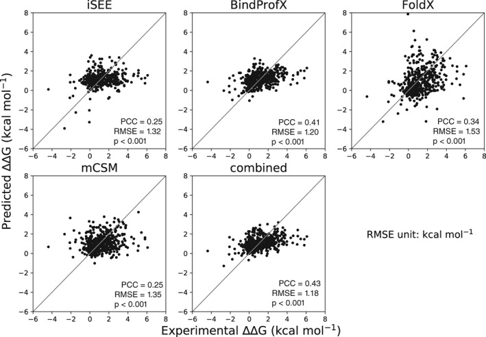
Correlations between predicted and experimental ΔΔG for various ΔΔG predictors tested on 487 mutations of SKEMPI 2.0. PCC is the Pearson's correlation coefficient, P is two tailed P value of PCC, and RMSE represents root mean squared error

To see if a combination of those ΔΔG predictors could improve the prediction performance, we simply averaged their predictions. The resulting combined predictor outperforms all the individual predictors with improved RMSE (1.18 kcal/mol) and PCC (0.43) (Figure 4).

3.4. Feature importance

We analyzed the importance of iSEE features for the prediction performance. This was done by calculating the averaged decrease of mean squared error for splitting on a given feature over all trees in the random forest model (see Methods). The results (Figure 5) reveal that the PSSM value of the wildtype amino acid (PSSM_wt) and the difference of PSSM values between mutant and wildtype residues (PSSM_diff) are the two most important features. They capture the evolutionary conservation of a specific amino acid at the mutation position and its change after mutation, respectively. PSSM has been proven to provide crucial information in various related topics, such as binding site predictions37 and hot‐spot predictions.38 The alignment depth does not seem to have much impact on the prediction performance (Supporting Information Figure S4). However, with most entries having over 300 sequences in their alignment a more systematic study should be performed to come to clear conclusions on this. The next most important feature is an energetic term, namely the change in intermolecular electrostatic energy calculated by HADDOCK between the mutant and wildtype complexes (Eelec_diff), followed by the PSSM information content (PSSM_IC). The latter captures the evolutionary conservation over all 20 types of amino acids that can potentially appear at the mutation position. The high importance of the PSSM_wt, PSSM_diff, and PSSM_IC features indicate that evolutionary conservation is essential to quantitatively describe the effect of mutations on binding affinity.

Figure 5.

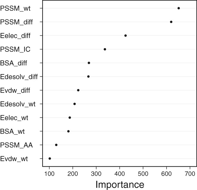
iSEE feature importance analysis. The importance value is measured as the decrease of mean squared prediction error when splitting on a given feature, averaged over all trees. The higher its value, the more important is the corresponding feature. The PSSM profile scores for the 20 amino acids are presented as a group in “PSSM_AA”

3.5. Case study: The MDM2–P53 complex

The effect of several new mutations in the complex of MDM2 with the tumor suppressor protein p53, which plays a central role in cancer development,39, 40 was characterized experimentally in our laboratory using a novel high‐throughput binding assay (van Rossum et al, manuscript in preparation). It contains ΔΔG measurements for 33 new mutations, 7 of which have reached the experimental detection limit (Supporting Information Table S8). The average experimental error for this dataset was estimated to be less than 0.5 kcal/mol. Like the performance on S487 dataset, the predictors have difficulties in predicting ΔΔG for this complex with all PCC values below 0.40 with P values ranging from .070 to .491(Supporting Information Figure S5). If we treat the problem as a classification one to see how well they detect important mutations with ΔΔG ≥ 2 kcal/mol. iSEE reliably identified important mutations (ΔΔG ≥ 2 kcal/mol) with the highest Matthews correlation coefficient (MCC) of 0.61 together with FoldX (Supporting Information Table S1).

We further performed a full computational mutation scanning of the interface of the MDM2–p53 complex: Each interface residue in the complex (26 and 12 residues for MDM2 and p53, respectively) was mutated to all other 19 amino acid types (Figure 6). Only single point mutations were considered. In total, we thus conducted 722 computational mutations, of which 33 have experimental measurements. None of the predicted ΔΔG values was negative, which indicates that no interface mutations were predicted to strengthen the interaction between MDM2 and p53. This is largely consistent with the experimental data: Experimentally only six mutations were found to stabilize the complex, but only by very small amounts (≥ −0.4 kcal/mol, Supporting Information Table S8). Considering the RMSE of iSEE (1.41 kcal/mol) predicting those is challenging.

Figure 6.

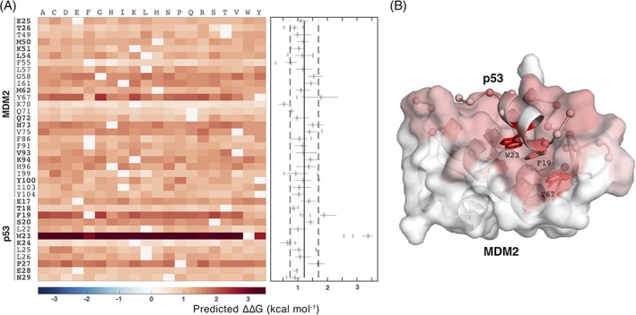
Full computational mutation scanning of the MDM2–p53 interface using iSEE. A, Heat map of ΔΔG values for the mutation of each residue in the MDM2–p53 interface to all other amino acid types. The sites with at least one experimental mutation are indicated in bold. Mutations from one amino acid to the same amino acid were assigned a value of zero. The right panel shows the distribution of ΔΔG values for each site with the vertical solid line and dashed lines showing the average and standard deviations of all predicted ΔΔG values, respectively. Three residues have their median above the average + one standard deviations showing more sensitivity to mutations. Two of those are experimentally validated hot‐spots (W23 and F19). B, the three predicted key binding sites are represented in sticks and all 38 interface sites in ball in the 3D structure of MDM2–p53 complex (PDB ID: 1YCR). MDM2 is represented in cartoon and surface and p53 in cartoon. Each interface site is colored by the median of full mutational predictions

From Figure 6, we can clearly identify three residues more sensitive to mutations: Y67 on MDM2 and F19 and W23 on p53. The latter two are experimental hot‐spots41 (Supporting Information Tables S2 and S8) and the third one is a candidate for experimental verification.

4. DISCUSSION

We have developed a machine learning based ΔΔG predictor, iSEE, for quantitative prediction of the effects of single point mutations at the interface of a protein–protein complex. By combining structural, evolutionary, and energetic features and training on a large and diverse dataset, our iSEE predictor not only demonstrated a consistent and high performance on various types of mutations during training, but also competed with state‐of‐the‐art methods (based on empirical potential or machine learning models) on independent blind test datasets.

Compared with other machine learning methods, our predictor uses a rather small number of features, 31 in total which minimize the risk of overfitting (mCSM, eg, could use over 100 features). Evolutionary features, which benefit from the wealth of sequence data, are particularly sensitive to describe the impact of mutations on binding affinity as demonstrated by our feature importance analyses. The evolutionary conservation at both the amino acid type level (PSSM_wt and PSSM_diff) and mutation position level (PSSM_IC) were dominant among all iSEE features. Next to evolutionary features, energetic terms calculated with HADDOCK contribute to a quantitatively prediction of ΔΔGs, in particular the change of intermolecular electrostatic energy (Eelec_diff).

Unlike mCSM for which only wild‐type structures are needed as input, iSEE does require the structures of both wildtype and mutant complexes. Models of the mutant complexes were obtained using the HADDOCK refinement server.29 The robust prediction results for mutations in loop versus non‐loop and mutations with different residue size changes indicates that this approach—the short refinement in explicit solvent performed by HADDOCK—can handle a small degree of conformational changes and remove steric clashes. To explore whether using an ensemble of structural models instead of a single model would improve the prediction performance, we also trained and tested iSEE using the average features calculated from the top four models returned by the HADDOCK refinement server. iSEE seems rather robust with respect to small conformational differences that might affect the energetic terms since using values from the top‐ranked model or averages over the best 4 does not have any significant impact on its performance (Supporting Information Table S3). More systematic analyses are, however, needed to draw solid conclusions on this point.

With the recent release of SKEMPI 2.0, it becomes possible to benchmark current ΔΔG predictors on a large and novel blind dataset. Our benchmarking results on a set of 487 mutations show that all state‐of‐the‐art ΔΔG predictors do not perform well with PCCs lower than 0.42. This indicates there is still a plenty of room for further improvements. Interestingly, averaging the predictions from the different ΔΔG predictors generated an improved prediction performance, indicating the various ΔΔG predictors might use complementary features. This should be useful for further development and improvement of ΔΔG predictors.

Supporting information

supporting Information

Geng C, Vangone A, Folkers GE, Xue LC, Bonvin AMJJ. iSEE: Interface structure, evolution, and energy‐based machine learning predictor of binding affinity changes upon mutations. Proteins. 2019;87:110–119. 10.1002/prot.25630

REFERENCES

- 1. Wang X, Wei X, Thijssen B, Das J, Lipkin SM, Yu H. Three‐dimensional reconstruction of protein networks provides insight into human genetic disease. Nat Biotechnol. 2012;30(2):159‐164. [DOI] [PMC free article] [PubMed] [Google Scholar]
- 2. Zhou M, Li Q, Wang R. Current experimental methods for characterizing protein–protein interactions. Chem Med Chem. 2016;11(8):738‐756. [DOI] [PMC free article] [PubMed] [Google Scholar]
- 3. Kastritis PL, Bonvin AMJJ. On the binding affinity of macromolecular interactions: daring to ask why proteins interact. J R Soc Interface. 2012;10(79):20120835‐20120835. [DOI] [PMC free article] [PubMed] [Google Scholar]
- 4. Steinbrecher T, Abel R, Clark A, Friesner R. Free energy perturbation calculations of the thermodynamics of protein side‐chain mutations. J Mol Biol. 2017;429(7):923‐929. [DOI] [PubMed] [Google Scholar]
- 5. Perthold JW, Oostenbrink C. Simulation of reversible protein‐protein binding and calculation of binding free energies using perturbed distance restraints. J Chem Theory Comput. 2017;13(11):5697‐5708. [DOI] [PMC free article] [PubMed] [Google Scholar]
- 6. Guerois R, Nielsen JE, Serrano L. Predicting changes in the stability of proteins and protein complexes: a study of more than 1000 mutations. J Mol Biol. 2002;320(2):369‐387. [DOI] [PubMed] [Google Scholar]
- 7. Dourado DFAR, Flores SC. A multiscale approach to predicting affinity changes in protein‐protein interfaces. Proteins Struct Funct Bioinform. 2014;82(10):2681‐2690. [DOI] [PubMed] [Google Scholar]
- 8. Benedix A, Becker CM, de Groot BL, Caflisch A, Böckmann RA. Predicting free energy changes using structural ensembles. Nat Methods. 2009;6(1):3‐4. [DOI] [PubMed] [Google Scholar]
- 9. Li M, Petukh M, Alexov E, Panchenko AR. Predicting the impact of missense mutations on protein–protein binding affinity. J Chem Theory Comput. 2014;10(4):1770‐1780. [DOI] [PMC free article] [PubMed] [Google Scholar]
- 10. Dehouck Y, Kwasigroch JM, Rooman M, Gilis D. BeAtMuSiC: prediction of changes in protein–protein binding affinity on mutations. Nucleic Acids Res. 2013;41(W1):W333‐W339. [DOI] [PMC free article] [PubMed] [Google Scholar]
- 11. Pires DEV, Ascher DB, Blundell TL. mCSM: predicting the effects of mutations in proteins using graph‐based signatures. Bioinformatics. 2013;30(3):335‐342. [DOI] [PMC free article] [PubMed] [Google Scholar]
- 12. Berliner N, Teyra J, Çolak R, Garcia Lopez S, Kim PM. Combining structural modeling with ensemble machine learning to accurately predict protein fold stability and binding affinity effects upon mutation Kurgan L, editor. PLoS One. 2014;9(9):e107353. [DOI] [PMC free article] [PubMed] [Google Scholar]
- 13. Brender JR, Zhang Y. Predicting the effect of mutations on protein‐protein binding interactions through structure‐based Interface profiles Jernigan RL, editor. PLoS Comput Biol. 2015;11(10):e1004494. [DOI] [PMC free article] [PubMed] [Google Scholar]
- 14. Moal IH, Fernández‐Recio J. SKEMPI: a structural kinetic and energetic database of mutant protein interactions and its use in empirical models. Bioinformatics. 2012;28(20):2600‐2607. [DOI] [PubMed] [Google Scholar]
- 15. Jankauskaite J, Jiménez‐García B, Dapkūnas J, Fernández‐Recio J, Moal IH. SKEMPI 2.0: an updated benchmark of changes in protein‐protein binding energy, kinetics and thermodynamics upon mutation. Bioinformatics. 2018;9:e1003216. [DOI] [PMC free article] [PubMed] [Google Scholar]
- 16. Moreira IS, Fernandes PA, Ramos MJ. Hot spots—a review of the protein–protein interface determinant amino‐acid residues. Proteins Struct Funct Bioinform. 2007;68(4):803‐812. [DOI] [PubMed] [Google Scholar]
- 17. DeLano WL. Unraveling hot spots in binding interfaces: progress and challenges. Curr Opin Struct Biol. 2002;12(1):14‐20. [DOI] [PubMed] [Google Scholar]
- 18. Martins SA, Perez MAS, Moreira IS, Sousa SF, Ramos MJ, Fernandes PA. Computational alanine scanning mutagenesis: MM‐PBSA vs TI. J Chem Theory Comput. 2013;9(3):1311‐1319. [DOI] [PubMed] [Google Scholar]
- 19. Xiong P, Zhang C, Zheng W, Zhang Y. BindProfX: assessing mutation‐induced binding affinity change by protein Interface profiles with pseudo‐counts. J Mol Biol. 2017;429(3):426‐434. [DOI] [PMC free article] [PubMed] [Google Scholar]
- 20. Hertz GZ, Stormo GD. Identifying DNA and protein patterns with statistically significant alignments of multiple sequences. Bioinformatics. 1999;15(7):563‐577. [DOI] [PubMed] [Google Scholar]
- 21. Dominguez C, Boelens R, Bonvin AMJJ. HADDOCK: a protein−protein docking approach based on biochemical or biophysical information. J Am Chem Soc. 2003;125(7):1731‐1737. [DOI] [PubMed] [Google Scholar]
- 22. Janin J, Henrick K, Moult J, et al. CAPRI: a critical assessment of PRedicted interactions. Proteins Struct Funct Bioinform. 2003;52(1):2‐9. [DOI] [PubMed] [Google Scholar]
- 23. Vangone A, Rodrigues JPGLM, Xue LC, et al. Sense and simplicity in HADDOCK scoring: lessons from CASP‐CAPRI round 1. Proteins Struct Funct Bioinform. 2017;85(3):417‐423. [DOI] [PMC free article] [PubMed] [Google Scholar]
- 24. Fernández‐Recio J, Totrov M, Abagyan R. Identification of protein–protein interaction sites from docking energy landscapes. J Mol Biol. 2004;335(3):843‐865. [DOI] [PubMed] [Google Scholar]
- 25. Breiman L. Random forests. Mach Learn. 2001;45(1):5‐32. [Google Scholar]
- 26. Liaw A, Wiener M. Classification and regression by randomForest. R News. 2002;2:18‐22. [Google Scholar]
- 27. Levy ED. A simple definition of structural regions in proteins and its use in analyzing Interface evolution. J Mol Biol. 2010;403(4):660‐670. [DOI] [PubMed] [Google Scholar]
- 28. Geng C, Vangone A, Bonvin AMJJ. Exploring the interplay between experimental methods and the performance of predictors of binding affinity change upon mutations in protein complexes. Protein Eng Des Select. 2016;29(8):291‐299. [DOI] [PubMed] [Google Scholar]
- 29. van Zundert GCP, Rodrigues JPGLM, Trellet M, et al. The HADDOCK2.2 web server: user‐friendly integrative modeling of biomolecular complexes. J Mol Biol. 2016;428(4):720‐725. [DOI] [PubMed] [Google Scholar]
- 30. Jorgensen WL, Tirado‐Rives J. The OPLS [optimized potentials for liquid simulations] potential functions for proteins, energy minimizations for crystals of cyclic peptides and crambin. J Am Chem Soc. 1988;110(6):1657‐1666. [DOI] [PubMed] [Google Scholar]
- 31. Altschul S. Gapped BLAST and PSI‐BLAST: a new generation of protein database search programs. Nucleic Acids Res. 1997;25(17):3389‐3402. [DOI] [PMC free article] [PubMed] [Google Scholar]
- 32. Kuhn M. Building predictive models in R using the caret package. J Stat Softw. 2008;28(1):1‐26.27774042 [Google Scholar]
- 33. Morin A, Eisenbraun B, Key J, et al. Cutting edge: collaboration gets the most out of software. eLife. 2013;2:e01456. [DOI] [PMC free article] [PubMed] [Google Scholar]
- 34. Kabsch W, Sander C. Dictionary of protein secondary structure: pattern recognition of hydrogen‐bonded and geometrical features. Biopolymers. 1983;22(12):2577‐2637. [DOI] [PubMed] [Google Scholar]
- 35. Harpaz Y, Gerstein M, Chothia C. Volume changes on protein folding. Structure. 1994;2(7):641‐649. [DOI] [PubMed] [Google Scholar]
- 36. Meyer PA, Socias S, Key J, et al. Data publication with the structural biology data grid supports live analysis. Nat Commun. 2016;7:ncomms10882. [DOI] [PMC free article] [PubMed] [Google Scholar]
- 37. Walia RR, Xue LC, Wilkins K, El‐Manzalawy Y, Dobbs D, Honavar V. RNABindRPlus: a predictor that combines machine learning and sequence homology‐based methods to improve the reliability of predicted RNA‐binding residues in proteins Kurgan L, editor. PLoS One. 2014;9(5):e97725. [DOI] [PMC free article] [PubMed] [Google Scholar]
- 38. Moreira IS, Koukos PI, Melo R, et al. SpotOn: high accuracy identification of protein‐protein Interface hot‐spots. Sci Rep. 2017;7(1):8007. [DOI] [PMC free article] [PubMed] [Google Scholar]
- 39. Wang S, Zhao Y, Aguilar A, Bernard D, Yang C‐Y. Targeting the MDM2–p53 protein–protein interaction for new cancer therapy: progress and challenges. Cold Spring Harb Perspect Med. 2017;7(5):a026245. [DOI] [PMC free article] [PubMed] [Google Scholar]
- 40. Arkin MR, Wells JA. Small‐molecule inhibitors of protein–protein interactions: progressing towards the dream. Nat Rev Drug Discov. 2004;3(4):301‐317. [DOI] [PubMed] [Google Scholar]
- 41. Bogan AA, Thorn KS. Anatomy of hot spots in protein interfaces. J Mol Biol. 1998;280(1):1‐9. [DOI] [PubMed] [Google Scholar]
Associated Data
This section collects any data citations, data availability statements, or supplementary materials included in this article.
Supplementary Materials