

ABSTRACT
The objective of the study was to suggest a novel quantitative assessment of acetabular bone defects based on a statistical shape model, validate the method, and present preliminary results. Two exemplary CT‐data sets with acetabular bone defects were segmented to obtain a solid model of each defect pelvis. The pathological areas around the acetabulum were excluded and a statistical shape model was fitted to the remaining healthy bone structures. The excluded areas were extrapolated such that a solid model of the native pelvis per specimen resulted (i.e., each pelvis without defect). The validity of the reconstruction was tested by a leave‐one‐out study. Validation results showed median reconstruction errors of 3.0 mm for center of rotation, 1.7 mm for acetabulum diameter, 2.1° for inclination, 2.5° for anteversion, and 3.3 mm3 for bone volume around the acetabulum. By applying Boolean operations on the solid models of defect and native pelvis, bone loss and bone formation in four different sectors were assessed. For both analyzed specimens, bone loss and bone formation per sector were calculated and were consistent with the visual impression. In specimen_1 bone loss was predominant in the medial wall (10.8 ml; 79%), in specimen_2 in the posterior column (15.6 ml; 46%). This study showed the feasibility of a quantitative assessment of acetabular bone defects using a statistical shape model‐based reconstruction method. Validation results showed acceptable reconstruction accuracy, also when less healthy bone remains. The method could potentially be used for implant development, pre‐clinical testing, pre‐operative planning, and intra‐operative navigation. © 2018 The Authors. Journal of Orthopaedic Research® Published by Wiley Periodicals, Inc. on behalf of Orthopaedic Research Society. J Orthop Res 9999:1–9, 2018.
Keywords: acetabular bone defects, quantification, statistical shape model, volume analysis
Severe acetabular bone defects are still challenging to quantify when it comes to revision total hip arthroplasty (THA). Numerous classification schemes have been proposed to categorize acetabular bone loss.1, 2, 3 However, these schemes mainly rely on visual interpretation of anatomical landmarks, which may lead to a poor inter‐observer reliability and intra‐observer repeatability.4, 5, 6 The reliability increases when using three‐dimensional (3D) computer tomography (CT) scans instead of 2D radiographs, but there still remains a bias related to subjective interpretation.5, 7, 8 Furthermore, the current classification schemes are mainly descriptive and hence it remains difficult to transfer them into pre‐clinical testing, implant development, and to anticipate the exact amount of bone loss in pre‐operative planning.9 Novel imaging techniques allow a 3D presentation of individual bone structures, but an objective and quantitative method to assess the bone defects is still not available.
Two of the most common acetabular defect classification schemes are the Paprosky classification3 and the American Academy of Orthopedic Surgeons (AAOS) classification.1 The Paprosky classification distinguishes bone defects according to possible treatment options, the AAOS classification according to their appearance as cavitary or segmental and their location. Within the classification schemes, the estimation of bone loss is often based on remaining anatomical landmarks, the contra‐lateral side, and/or the surgeons experience.10, 11, 12
However, it is often difficult to evaluate severe and/or bilateral bone defects without the native pelvic anatomy for comparison. A promising option to estimate the native anatomy is the application of a statistical shape model (SSM), which is a parametric model of a given training set of healthy pelvises.13, 14, 15 A SSM can be altered via a unique set of parameters to reconstruct the native pelvis (i.e., the pelvis without bone defect) on the basis of a defect pelvis (i.e., the pelvis with bone defect). Recently published studies showed the feasibility to estimate the native pelvis anatomy using a SSM and thereby allow a novel view on defect classification.9, 14, 15 Among the estimation of bone loss, also bone formation due to remodeling processes could be identified when comparing the defect pelvis with the native pelvis.
The aims of this study were to (1) suggest a method to objectively quantify acetabular bone defects in terms of bone loss and bone formation and to derive bone defect shape, (2) validate the accuracy of the applied reconstruction method, and (3) present preliminary results for two exemplary pelvises with acetabular bone defects.
MATERIALS AND METHODS
The suggested method consisted of four parts: Pre‐processing, reconstruction, sector definition, and analysis (Fig. 1). The pre‐processing included a CT‐scan, segmentation of bone structures, and creation of a solid model of the defect pelvis. The reconstruction included masking of the pathological regions around the acetabulum and the SSM‐based reconstruction of the native pelvis based on the remaining healthy bone. In the sector definition part, clinically relevant defect sectors were constructed on native pelvis and defect pelvis. In the analysis part, quantitative values for bone loss and bone formation were obtained and defect shape was derived.
Figure 1.
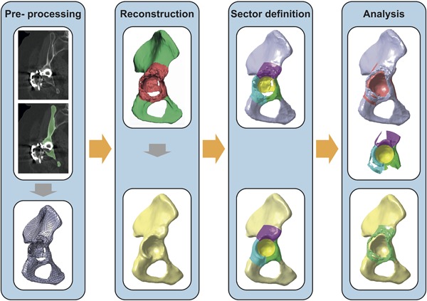
Workflow of the quantitative assessment. Determination of a solid model of the pelvis with bone defect on the basis of a segmented CT‐data set. Masking of the pathological regions and reconstruction based on the remaining healthy bone. Definition of clinically relevant bone defect sectors on defect pelvis and native pelvis. Analysis of bone volume loss (light red), bone defect shape, and bone formation (light green).
Pre‐processing
CT‐scans, conducted within the scope of pre‐operative planning, of two pelvises with exemplary acetabular bone defects were included in this study. Specimen 1 (female, 62 years) was kindly provided by the senior hip reconstruction surgeon FT and categorized as Paprosky IIIA. The revision of the existing acetabular reconstruction ring with a cemented cup was conducted due to aseptic loosening and superior medial migration. Specimen 2 (female, 77 years) was kindly provided by the senior hip reconstruction surgeon MR and categorized as Paprosky IIIA. The revision of the existing cementless hemispheric cup was conducted due to superior and posterior as well as lateral migration. The provision of the CT‐scans was approved by the LMU Munich ethics committee (Project No. 18‐108 UE). The CT‐scans had a slice thickness of 3 mm and a pixel size of 0.78 mm.
Segmentation of bone structures was performed in Mimics (Materialise NV, Leuven, Belgium). Since metal implants were present in the CT‐scans an accurate automatic segmentation was prevented. Therefore, the segmentation was conducted manually by RS under supervision of an experienced radiologist. The resulting three‐dimensional surface of the defect pelvis was smoothed with factor 0.75 and 5 iterations and exported as standard triangulation language (STL) mesh.
After mesh correction in 3‐matic (Materialise NV, Leuven, Belgium), the STL files were further processed in Geomagic Design X (3Dsystems, Rock Hill, SC). A mesh optimization algorithm was applied, followed by the transformation into a solid body using auto surfacing. The result was a solid model of the defect pelvis, which could be further processed in the CAD (computer aided design) software CATIA V5 (Dassault Systèmes, Vélizy‐Villacoublay Cedex, France). Volume difference between STL and solid model was 0.24% and 0.25%, respectively.
Reconstruction
In order to reconstruct the native pelvis with a SSM, all pathological areas had to be excluded. Therefore, the pathological areas around the acetabulum were masked for each pelvis individually in order to preserve as much healthy bone structures as possible.
The SSM was trained on the basis of 66 CT‐data sets, which were kindly provided by the radiological department of the Charité Berlin, and already used in previous studies.16, 17, 18 The number of CT‐data sets included in this study exceeded the amount of data sets required to capture the intrinsic shape variations in the native pelvis.19 No known pathology or symptoms of the lumbar spine, pelvis or acetabulum were present and the patients were scanned for clinical, non‐orthopedic indications. Voxel size in x–y direction was between 0.7 and 0.8 mm and in z‐ direction 4 mm or smaller.
The 66 CT‐data sets were segmented. Based on this training set, a shape model was created which contains 65 modes of shape variation. These modes represent the geometric variation occurring in the training population sorted by its magnitude, that is, mode 1 encodes the largest and mode 65 the smallest geometric deformation. By fitting the SSM to remaining healthy bone structures, the excluded pathological areas could be extrapolated plausibly.20
Sector Definition
In order to relate the bone defects to areas of clinical relevance, four defect sectors were defined (Fig. 2). The defined sectors were cranial roof, anterior column, posterior column, and medial wall (Fig. 2A), which were inspired by previous studies.9, 21, 22 In order to consider patient‐specific anatomy, the sectors were constructed on the acetabular plane, aligned to the patient coordinate system, and scaled in relation to the acetabulum diameter (Fig. 2).
Figure 2.
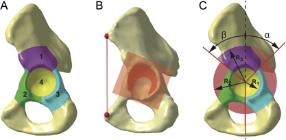
Bone defect sectors. (A) Defect sectors are cranial roof (1), anterior column (2), posterior column (3), and medial wall (4). (B) Defect sectors are constructed on the acetabular plane and aligned to the patient coordinate system. (C) Defect sectors are scaled in relation to the acetabulum diameter using the parameters R 1, R 2, and R 3 as well as angles α and β.
The acetabular plane was defined by the acetabular rim under exclusion of the acetabular notch (Fig. 2B).23 The anterior pelvic plane, given by left and right Anterior Superior Iliac Spine (l‐ASIS and r‐ASIS) as well as the center between left and right Pubic Tubercle (l‐PT and r‐PT), defined the frontal plane of the coordinate system. Transversal plane was parallel to the line between l‐ASIS and r‐ASIS and perpendicular to the frontal plane, sagittal plane resulted thereof. The landmarks were defined by the most ventral points in each region, which correspond to the contact points with a virtual plane.23, 24 Acetabulum diameter (AcD) and center of rotation (CoR) were determined by a sphere fitting procedure on the joint contact area (Fig. 2B).15, 25
The defect sectors were constructed parametrically (Fig. 2C), whereby the medial wall radius (R 1) was defined by 0.87 times AcD, caudal borders of posterior and anterior columns (R 2) were defined by 1.90 times AcD, and superior border of cranial roof (R 3) was defined by 2.2 times AcD. The subdivision of the sectors was defined by the angles α (45)° and β (50°) with respect to the frontal plane. The depth of the sectors was defined by 2.0 times AcD (not shown).
Analysis
Based on the solid models of defect pelvis, native pelvis, and the defect sectors, a quantitative analysis of acetabular bone defects in each sector was performed. Both solid models were imported and superimposed in CATIA V5 and divided into the four sectors. By means of Boolean operations, bone loss and bone formation could be assessed (Fig. 3). Subtracting defect pelvis from native pelvis resulted in a body that represents bone loss (Fig. 3A). Subtracting native pelvis from defect pelvis resulted in a body that represents bone formation (Fig. 3B). Bone loss and bone formation were analyzed for each sector individually in terms of absolute values and relative to bone volume of the native pelvis in the corresponding sector. Furthermore, overall defect shape and defect shape within each sector were obtained.
Figure 3.
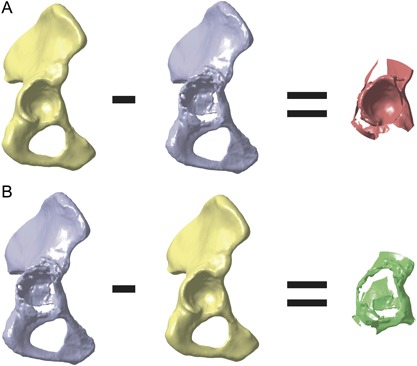
Calculation of bone loss and bone formation. (A) Subtracting defect pelvis from native pelvis results in a body that represents bone loss. (B) Subtracting native pelvis from defect pelvis results in a body that represents bone formation.
Validation of the Reconstruction Method
The SSM‐based reconstruction method was validated by means of a Leave‐one‐out study. Thereby, one pelvis at a time was removed from the 66 pelvises and reconstructed using a SSM consisting of the remaining 65 pelvises. The validity of the reconstruction was assessed by comparing each original pelvis with its reconstruction. In order to replicate clinical CT‐data sets, four scenarios of absent bone structures were realized by different masks (Fig. 4A,B). In the first scenario, no mask was applied to obtain the representation accuracy of one individual pelvis by the SSM, that is, the ground truth (Scenario_0 and Mask_0). One excluded acetabulum represented the second scenario in which an implant and/or bone defect was masked unilaterally with an intact opposite side (Scenario_1 and Mask_1). Two masked acetabuli represented a scenario in which an implant and/or a bone defect was present on both sides (Scenario_2 and Mask_2). Incomplete scans of the os ilium in combination with an implant and/or bone defect on both sides represented the worst‐case scenario for reconstruction within this study (Scenario_3 and Mask_3).
Figure 4.
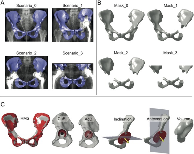
Validation of the statistical shape model. The validation comprises a Leave‐one‐out study representing four clinical scenarios (Scenario_0, Scenario_1, Scenario_2, Scenario_3) by four masks (Mask_0, Mask_1, Mask_2, Mask_3) and comparing six anatomical parameters. (A) Scenario_0 represents ground truth of the reconstruction. Scenario_1 represents a scenario in which an implant and/or bone defect on one side is masked and excluded before the reconstruction. Scenario_2 represents a scenario in which both acetabuli are excluded. Scenario_3 represents a scenario in which both acetabuli and the cranial areas of the os ilium are excluded due to an incomplete CT‐scan. (B) Parametrical masks were constructed for each scenario. (C) Parameters used to asses the quality of the reconstruction are root‐mean‐square of surface deviation (RMS), position of center of rotation (CoR), diameter of acetabulum (AcD), anatomical inclination (Inclination), anatomical anteversion (Anteversion), and bone volume within the left acetabulum mask (Volume).
The mask around the acetabulum was defined by two spheres. Sphere one covered the acetabulum with a diameter of 2.05 times AcD and sphere two covered the spina ischiadica with a diameter of 0.33 times AcD. The mask of the cranial parts of the os ilium was defined by a plane parallel to the transversal plane with an offset of 0.35 times AcD with respect to the ASIS‐landmarks in cranial direction.
The reconstruction error between each original pelvis and its reconstruction was analyzed based on six parameters (Fig. 4C): Root‐mean‐square (RMS) of surface deviation, distance between CoR positions, absolute difference in AcD, absolute difference in anatomic inclination and anteversion according to Murray,26 and absolute difference in volume within the acetabulum mask.
The effect of different numbers of shape variation modes used in the SSM and the effect of different mask sizes were assessed within this validation. Reconstruction error was assessed based on the left acetabulum.
RESULTS
Validation Results
Number of shape variation modes affected the reconstruction error, exemplary shown for Mask_2 (Fig. 5). Mean and percentile values of the reconstruction errors decreased when the number of shape variation modes were increased from 0 to 20, but remained almost constant for higher numbers of shape variation modes. Maximum reconstruction errors were lowest for the SSM with 10 or 20 shape variation modes.
Figure 5.
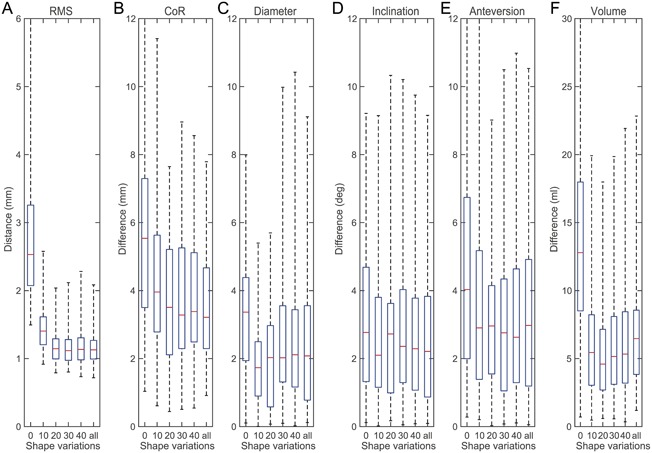
Reconstruction errors of Mask_2 using SSMs with different numbers of shape variation modes. Shown are distance and differences between each individual pelvis and its reconstruction using the scaled mean shape (0), 10 shape variation modes (10), 20 shape variation modes (20), 30 shape variation modes (30), 40 shape variation modes (40), and 65 shape variation modes (all). (A) RMS of surface deviation. (B) CoR position. (C) Acetabulum diameter. (D) Inclination. (E) Anteversion. (F) Bone volume within acetabulum mask. The boxplots show median, 25% and 75% percentile, and extreme values including all outliers.
Reconstruction errors with respect to different mask sizes were analyzed based on the SSM with 20 shape variation modes (Fig. 6). The RMS constantly increased with increasing mask sizes (Fig. 6A). In contrast, the reconstruction error of CoR, AcD, inclination, anteversion, and volume increased noticeably from Mask_0 to Mask_1, but only slightly increased or remained constant with a further increase in mask sizes (Fig. 6B–F).
Figure 6.
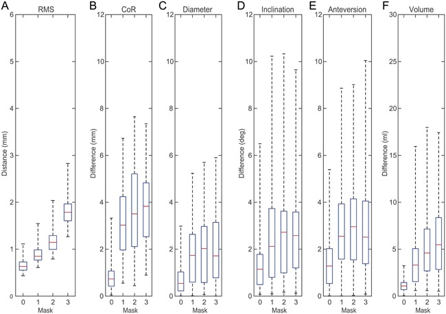
Reconstruction errors of the SSM with 20 shape variation modes using different masks. Shown are distance and differences between each individual pelvis and its reconstruction using Mask_0 (0), Mask_1 (1), Mask_2 (2), and Mask_3 (3). (A) RMS of surface deviation. (B) CoR position. (C) Acetabulum diameter. (D) Inclination. (E) Anteversion. (F) Bone volume within acetabulum mask.
Quantitative Defect Assessment
The suggested method was successfully applied on two exemplary specimens (see Materials and Methods section) using the SSM with 20 shape variation modes (Fig. 7A). Bone volume of native pelvis and defect pelvis was calculated for each sector (brown and gray bars in Fig. 7B). Bone volume loss was calculated and expressed as absolute values (red bars in Fig. 7B) and additionally relative to the volume of the native pelvis in the corresponding sector (blue dots in Fig. 7B). Bone formation was calculated and expressed in terms of absolute values (green bars in Fig. 7B).
Figure 7.
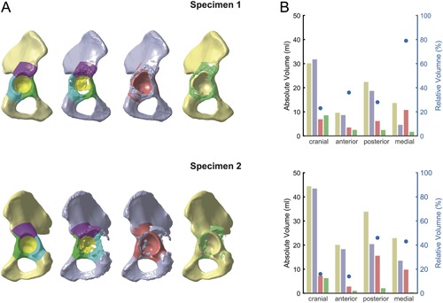
Quantitative defect assessment. (A) Native pelvis, defect pelvis, bone loss and bone formation of two exemplary specimens. (B) Volume of native pelvis (brown bars), defect pelvis (gray bars), bone loss (red bars are absolute values, blue dots are relative values), as well as bone formation (green bars) for each sector.
For both specimens, the results of the quantitative assessment of bone loss in each sector were consistent with the visual impression. In specimen 1, the medial sector seemed to be the most affected, which was reflected by a bone loss in this sector of 79% (10.8 ml), whereas bone loss was much lower in the three other sectors, namely 23% (6.9 ml) in the cranial roof, 36% (3.5 ml) in the anterior column and 28% (6.2 ml) in the posterior column. In specimen 2, a combined defect of posterior column and medial wall was reflected by a bone loss of 46% (15.6 ml) in the posterior column and of 43% (9.8 ml) in the medial wall, whereas cranial roof and anterior column only showed a bone loss of 16% (7.2 ml) and 14% (2.8 ml), respectively.
Furthermore, a considerable amount of bone formation was observed, which occurred mainly in the cranial roof. In this sector, bone formation in specimen 2 was 6.3 ml and in specimen 1 it even exceeded the amount of bone loss (8.6 ml vs. 6.9 ml).
DISCUSSION
Traditionally, acetabular bone defects were analyzed on the basis of 2D radiographs and categorized according to a specific classification scheme. Nowadays, 3D imaging techniques and virtual anatomical reconstruction using a SSM allow novel views on acetabular bone defect analysis. This study suggested and validated a method to quantify acetabular bone loss and bone formation, and to derive bone defect shape. These information could potentially be used for implant development, pre‐clinical testing, pre‐operative planning, and intra‐operative navigation.
The reconstruction method was validated using a Leave‐one‐out study on virtually created, clinically relevant bone defects and six parameters. In the first validation step, the influence of the number of shape variation modes was analyzed. The reconstruction error was highest with 0 shape variation modes (i.e., the mean scaled pelvis shape) and decreased when more shape variation modes were included in the SSM. This observation showed a statistical inference from the remaining bone structures to the absent bone structures which exceed the pure mean and scaled shape. The mean and percentile values of the reconstruction error decreased from 0 to 20 shape variation modes and were almost constant for higher number of shape variation modes (Fig. 5A). This indicated that the first 20 shape variation modes cover most of the anatomical variations of the pelvis. More shape variation modes did not necessarily improve the reconstruction quality, which is in good accordance to the findings of Vanden Berghe et al., who stated that 20 shape variations cover 95% of the anatomic variations.15
The extreme values of the reconstruction error including all outliers are crucial for a clinical application of the method. The extreme values were lowest for 10 and 20 shape variation modes and increased with higher and lower numbers of shape variation modes. In order to obtain a robust reconstruction method, the SSM was therefore limited in the consecutive steps to 20 shape variation modes.
The influence of different mask sizes on the reconstruction error was analyzed in the second validation step (Fig. 6). Only RMS constantly increased with increasing masks size (Fig. 6A), whereas the reconstruction errors of the anatomical parameters were lowest for Mask_0 and almost similar for Mask_1, Mask_2, and Mask_3 (Fig. 6B‐F). The RMS is the only parameter which considers the whole pelvis anatomy, such that an increasing amount of absent bone structures directly affects the RMS. In contrast, the anatomical parameters were derived only from the left acetabulum. Bone structures in this region were already excluded in Mask_1, a further increase in mask size by additional exclusion of the right acetabulum or cranial parts of the os ilium, therefore, only slightly affected the anatomical parameters. Median reconstruction error for Mask_1 was 3.0 mm for CoR, 1.7 mm for AcD, 2.1° for inclination, 2.5° for anteversion, and 3.3 mm3 for volume. The reconstruction results of the method applied in this study, are clearly superior to manual methods27, 28 and comparable to other SSM‐based reconstruction methods.14, 15 Since the presented method can be applied to CT‐data sets where both acetabuli are defect, the method is also superior to reconstruction methods using the contralateral hemi‐pelvis.12
To the authors' knowledge, this is the first study considering different clinically relevant scenarios in the validation of a SSM‐based reconstruction. Particularly, the reconstruction using Mask_3, where both acetabuli and large areas of the pelvis are excluded (Fig. 4B), could provide desirable guidance for the surgeons in such severe scenarios.
However, a maximum reconstruction error of approximately 10 mm in CoR position and acetabulum diameter, and of approximately 10° in inclination and anteversion has to be considered cautiously in clinical applications. Further investigations on the SSM could increase the reconstruction quality, for example by investigating a possible correlations between the appearance of outliers and the reconstruction quality of the remaining bone.
Feasibility of the presented defect quantification workflow was shown by analyzing two exemplary pelvises with acetabular bone defects. It was possible to dedicate bone loss in terms of absolute and relative values to the corresponding defect sector. Furthermore, bone formation due to remodeling processes was dedicated to the corresponding sector. In both specimens, the visual impression of bone loss was consistent with the numerical values. These values could provide a basis for a quantitative and objective defect classification, for example, by separating the specimens on the basis of thresholds in each sector. These quantitative measures should then be complemented by clinical measures, such as quality, thickness, and continuity of the remaining bone and possible implant fixation strategies.
The presented method has some limitations. First, the presence of metal implants lead to artifacts in the images which are caused by a combination of beam hardening, photon starvation, scatter, and edge effects.21, 29, 30 These artefacts may have detrimental effects on segmentation accuracy and demanded a manual segmentation under supervision of an experienced radiologist. The second limitation is the focus on quantitative measure of volume, whereby other important parameters yet remain unconsidered in the analysis. Further studies should complement the quantitative volume measures by additional measures, such as bone quality, bone thickness, ovality of acetabulum, weighting of defect zones depending on importance for load transfer, and potential discontinuity to allow inferences on treatment and implant fixation strategy. And the third main limitation is that in cases where pronounced individual anatomical characteristics were masked and excluded, the SSM was not able to reconstruct it accurately and large maximum reconstruction errors resulted. However, to the authors knowledge there is no better solution available, since it is currently impossible to infer from remaining bone structures to masked and excluded idiosyncracies.
In future, the presented method could potentially be used in scientific, clinical, and engineering applications. In science, the method could improve the assignment into defect categories, which in turn could increase the reliability of inter‐patient comparisons. Further studies should include a larger number of defect pelvises in order to obtain quantitative measures of acetabular bone defects, which could then be used as a basis for a classification scheme. In clinic routine, the method could be automated and provided within a pre‐operative planning software such that the surgeon is able to anticipate the treatment strategy and the required amount of material to fill the bone defect. Furthermore, since SSMs of the pelvis have already been used for example to estimate cup orientation or pelvic shape based on 2D anteroposterior radiographs,31, 32 the method could also be applied using 2D radiographs, such that a CT‐scan is not a mandatory prerequisite for the analysis. Finally, the method could be used to develop novel implant and treatment concepts, such as next generation patient‐specific implants9, 33, 34 and could be applied in pre‐clinical “in‐vitro” and “in silico” testing.35
AUTHORS' CONTRIBUTIONS
The authors GH, RS, HR, and TG worked on research design, image processing, validation, analysis and interpretation of data, as well as drafting and critically revising the manuscript. HG, VJ, MR, and FT provided the clinical data sets, worked on research design, checked the analysis and results for clinical plausibility, and critically revised the manuscript. All authors have read and approved the final submitted manuscript.
ACKNOWLEDGMENTS
The authors would like to thank Dr. med. Rudolf Schierjott for his support in the segmentation of the CT‐data sets, PD Dr. med. Patrick Weber for providing clinical CT‐data sets with acetabular defects, PD Dr. med. Stephan Tohtz, and the Charité Berlin for providing the CT‐data sets included in the Statistical Shape Model.
Conflicts of Interest: Three of the authors (GH, RS, TG) are employees of Aesculap AG Tuttlingen, a manufacturer of orthopedic implants. One author (HR) is employee of 1000shapes GmbH, a company for image and geometry processing. Four of the authors (HG, VJ, MR, FT) are advising surgeons in Aesculap R&D projects.
REFERENCES
- 1. D'Antonio JA, Capello WN, Borden LS, et al. 1989. Classification and management of acetabular abnormalities in total hip arthroplasty. Clin Orthop Relat Res 243:126–137. [PubMed] [Google Scholar]
- 2. Saleh KJ, Holtzman J, Gafni A, et al. 2001. Reliability and intraoperative validity of preoperative assessment of standardized plain radiographs in predicting bone loss at revision hip surgery. J Bone Joint Surg Am 83‐A:1040–1046. [DOI] [PubMed] [Google Scholar]
- 3. Paprosky WG, Perona PG, Lawrence JM. 1994. Acetabular defect classification and surgical reconstruction in revision arthroplasty. A 6‐year follow‐up evaluation. J Arthroplasty 9:33–44. [DOI] [PubMed] [Google Scholar]
- 4. Johanson NA, Driftmier KR, Cerynik DL, et al. 2010. Grading acetabular defects. The need for a universal and valid system. J Arthroplasty 25:425–431. [DOI] [PubMed] [Google Scholar]
- 5. Safir O, Lin C, Kosashvili Y, et al. 2012. Limitations of conventional radiographs in the assessment of acetabular defects following total hip arthroplasty. Can J Surg 55:401–407. [DOI] [PMC free article] [PubMed] [Google Scholar]
- 6. Engh CA, Sychterz CJ, Young AM, et al. 2002. Interobserver and intraobserver variability in radiographic assessment of osteolysis. J Arthroplasty 17:752–759. [DOI] [PubMed] [Google Scholar]
- 7. Walde TA, Mohan V, Leung S, et al. 2005. Sensitivity and specificity of plain radiographs for detection of medial‐wall perforation secondary to osteolysis. J Arthroplasty 20:20–24. [DOI] [PubMed] [Google Scholar]
- 8. Leung S, Naudie D, Kitamura N, et al. 2005. Computed tomography in the assessment of periacetabular osteolysis. J Bone Joint Surg Am 87:592–597. [DOI] [PubMed] [Google Scholar]
- 9. Horas K, Arnholdt J, Steinert AF, et al. 2017. Acetabular defect classification in times of 3D imaging and patient‐specific treatment protocols. Orthopaede 46:168–178. [DOI] [PubMed] [Google Scholar]
- 10. Perka C, Fink B, Millrose M, et al. 2012. Revisionsendoprothetik In: Claes L, Kirschner P, Perka C, Rudert M, editors. AE‐Manual der Endoprothetik. Heidelberg Dordrecht London New York: Springer; p 441–587. [Google Scholar]
- 11. Sporer SM. 2012. How to do a revision total hip arthroplasty: revision of the acetabulum. AAOS Instr Course Lect 61:303–311. [PubMed] [Google Scholar]
- 12. Gelaude F, Clijmans T, Broos PL, et al. 2007. Computer‐aided planning of reconstructive surgery of the innominate bone: automated correction proposals. Comput Aided Surg 12:286–294. [DOI] [PubMed] [Google Scholar]
- 13. Zachow S, Lamecker H, Elsholtz B, et al. 2005. Reconstruction of mandibular dysplasia using a statistical 3D shape model. Int Congr Ser 1281:1238–1243. [Google Scholar]
- 14. Krol Z, Skadlubowicz P, Hefti F, et al. 2013. Virtual reconstruction of pelvic tumor defects based on a gender‐specific statistical shape model. Comput Aided Surg 18:142–153. [DOI] [PubMed] [Google Scholar]
- 15. Vanden Berghe P, Demol J, Gelaude F, et al. 2017. Virtual anatomical reconstruction of large acetabular bone defects using a statistical shape model. Computer Methods Biomech Biomed Eng 20:577–586. [DOI] [PubMed] [Google Scholar]
- 16. Tohtz SW, Sassy D, Matziolis G, et al. 2010. CT evaluation of native acetabular orientation and localization: sex‐specific data comparison on 336 hip joints. Technol Health Care 18:129–136. [DOI] [PubMed] [Google Scholar]
- 17. Zahn RK, Grotjohann S, Pumberger M, et al. 2017. Influence of pelvic tilt on functional acetabular orientation. Technol Health Care 25:557–565. [DOI] [PubMed] [Google Scholar]
- 18. Zahn RK, Grotjohann S, Ramm H, et al. 2016. Pelvic tilt compensates for increased acetabular anteversion. Int Orthop 40:1571–1575. [DOI] [PubMed] [Google Scholar]
- 19. Chintalapani G, Ellingsen LM, Sadowsky O, et al. 2007. Statistical atlases of bone anatomy: construction, iterative improvement and validation. Proceedings of Medical Image Computing and Computer‐Assisted Intervention − MICCAI 2007. 10th International Conference, Brisbane, Australia, October 29 − November 2, 2007, Proceedings, Part I. Berlin Heidelberg: Springer; p 499‐506. [DOI] [PubMed]
- 20. Vidal‐Migallon I, Ramm H, Lamecker H. 2014. Reconstruction of partial liver shapes based on a statistical 3D shape model. Proc Shape Symp Delemont Switzerland 2015:22. [Google Scholar]
- 21. Gelaude F, Clijmans T, Delport H. 2011. Quantitative computerized assessment of the degree of acetabular bone deficiency: total radial acetabular bone loss (TrABL). Adv Orthop 2011:1–12. [DOI] [PMC free article] [PubMed] [Google Scholar]
- 22. Wassilew GI, Janz V, Perka C, et al. 2017. Defektadaptierte azetabulaere versorgung mit der trabecular‐metal‐technologie. Orthopaede 46:148–157. [DOI] [PubMed] [Google Scholar]
- 23. Higgins SW, Spratley EM, Boe RA, et al. 2014. A novel approach for determining three‐dimensional acetabular orientation: results from two hundred subjects. J Bone Joint Surg Am 96:1776–1784. [DOI] [PubMed] [Google Scholar]
- 24. Seim H, Kainmueller D, Heller M, et al. Automatic extraction of anatomical landmarks from medical image data: An evaluation of different methods. Proceedings of the 2009 IEEE International Symposium on Biomedial Imaging: From Nano to Macro. Boston, MA, USA; p 538–541.
- 25. Costin S, Micu CA, Mustata C, et al. 2013. Selection of methods for determining the rotation center of the hip articulation for the design of a custom acetabular prosthesis. Advances in Production, Automation and Transportation Systems. Proceedings of the 6th International Conference on Manufacturing Engineering, Quality and Production Systems (MEQAPS 2013), Proceedings of the 4th International Conference on Automotive and Transportation Systems (ICAT 2013) Brasov, Romania, June 1–3, 2013: WSEAS Press; p 294‐299.
- 26. Murray DW. 1993. The definition and measurement of acetabular orientation. J Bone Joint Surg Br 75:228–232. [DOI] [PubMed] [Google Scholar]
- 27. Bosker BH, Verheyen CCPM, Horstmann WG, et al. 2007. Poor accuracy of freehand cup positioning during total hip arthroplasty. Arch Orthop Trauma Surg 127:375–379. [DOI] [PMC free article] [PubMed] [Google Scholar]
- 28. Jolles BM, Genoud P, Hoffmeyer P. 2004. Computer‐assisted cup placement techniques in total hip arthroplasty improve accuracy of placement. Clin Orthop Relat Res 426:174–179. [DOI] [PubMed] [Google Scholar]
- 29. Huang JY, Kerns JR, Nute JL, et al. 2015. An evaluation of three commercially available metal artifact reduction methods for CT imaging. Phys Med Biol 60:1047–1067. [DOI] [PMC free article] [PubMed] [Google Scholar]
- 30. Barrett JF, Keat N. 2004. Artifacts in CT. Recognition and avoidance. Radiographics 24:1679–1691. [DOI] [PubMed] [Google Scholar]
- 31. Zheng G, von Recum J, Nolte LP, et al. 2012. Validation of a statistical shape model‐based 2D/3D reconstruction method for determination of cup orientation after THA. Int J Comput Assist Radiol Surg 7:225–231. [DOI] [PubMed] [Google Scholar]
- 32. Ehlke M, Ramm H, Lamecker H, et al. 2013. Fast generation of virtual X‐ray images for reconstruction of 3D anatomy. IEEE Trans Vis Comput Graph 19:2673–2682. [DOI] [PubMed] [Google Scholar]
- 33. Baauw M, van Hellemondt GG, van Hooff ML, et al. 2015. The accuracy of positioning of a custom‐made implant within a large acetabular defect at revision arthroplasty of the hip. Bone Joint J 97‐B:780–785. [DOI] [PubMed] [Google Scholar]
- 34. Wyatt MC. 2015. Custom 3D‐printed acetabular implants in hip surgery—innovative breakthrough or expensive bespoke upgrade? Hip Int 25:375–379. [DOI] [PubMed] [Google Scholar]
- 35. Kluess D, Wieding J, Souffrant R, et al. 2012. Finite element analysis in orthopaedic biomechanics In: Moratal D, editor. Finite element analysis. from biomedical applications to industrial developments. London: InTechOpen Limited; p 151–170. [Google Scholar]