A map of constrained coding regions in the human genome

Abstract

Deep catalogs of genetic variation from thousands of humans enable the detection of intraspecies constraint by identifying coding regions with a scarcity of variation. While existing techniques summarize constraint for entire genes, single gene-wide metrics conceal regional constraint variability within each gene. Therefore, we have created a detailed map of constrained coding regions (CCRs) by leveraging variation observed among 123,136 humans from the Genome Aggregation Database. The most constrained CCRs are enriched for pathogenic variants in ClinVar and mutations underlying developmental disorders. CCRs highlight protein domain families under high constraint and suggest unannotated or incomplete protein domains. The highest-percentile CCRs complement existing variant prioritization methods when evaluating de novo mutations in studies of autosomal dominant disease. Finally, we identify highly constrained CCRs within genes lacking known disease associations. This observation suggests that CCRs may identify regions under strong purifying selection that, when mutated, cause severe developmental phenotypes or embryonic lethality.

During World War II, Abraham Wald and the Statistical Research Group optimized the placement of scarce metal reinforcements on Allied planes based on the patterns of bullet holes observed over many sorties. Wald famously invoked the principles of survival bias to infer that armor should be placed where bullet damage was unobserved, since the observed damage came solely from planes that returned from their missions. Wald reasoned that planes that had been shot down likely took on critical damage in such locations¹.

Employing similar logic, we sought to identify localized, highly constrained coding regions (CCRs) in the human genome. We were motivated by the idea that the absence of genetic variation in coding regions (for example, one or more exons or portions thereof) ascertained from large human cohorts implies strong purifying selection owing to essential function or disease pathology. An intuitive approach to identifying intraspecies genetic constraint in human coding genes is to identify gene sequences that harbor no genetic variation or significantly less variation than expected. For example, Petrovski et al.² used genetic variation observed among 6,515 exomes in the National Heart, Lung, and Blood Institute Exome Sequencing Project dataset³ to develop the Residual Variation Intolerance Score (RVIS), which ranks genes by their intolerance to ‘protein-changing’ (that is, missense or loss-of-function and coding) variation. Similarly, Lek et al.⁴ integrated variation observed among 60,706 exomes in the Exome Aggregation Consortium (ExAC) to estimate each gene’s probability of loss-of-function intolerance (pLI), with genes having the highest pLI harboring significantly less loss-of-function variation than predicted⁵.

While existing gene-wide measures of constraint are effective for disease variant interpretation, metrics that yield a single score for an entire gene inherently cannot capture the variability in regional constraint that exists within protein-coding genes. Constraint variability is expected given that some regions encode conserved domains^6–10 critical to protein structure or function, while others encode polypeptides that are more tolerant to perturbation. Therefore, while useful, single gene-wide metrics such as pLI are susceptible to both overestimating (Fig. 1a) and underestimating (Fig. 1b) local constraint within genes exhibiting finer-scale variation in constraint. Consequently, they are incapable of highlighting the subset of critical regions within each gene that are under the greatest selective pressure (Fig. 1, regions highlighted in red). This manuscript presents a detailed map of CCRs in human genes, with a focus on identifying coding regions predicted to be under the highest constraint. We demonstrate that the most constrained regions recover known disease loci, assist in the prioritization of de novo mutation, and illuminate new genes that may underlie previously unknown disease phenotypes.

Fig. 1. Gene-wide summary measures of constraint are prone to overstating and understating constraint within specific regions of protein-coding genes.

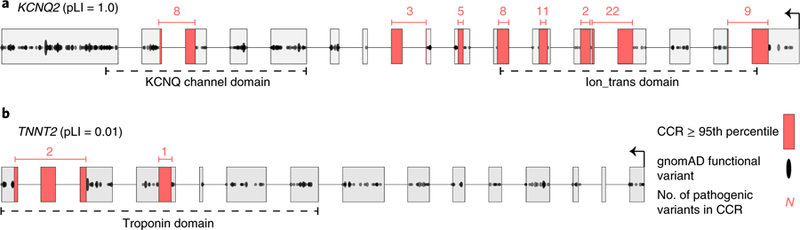
a, KCNQ2 has the highest possible pLI score of 1.0, yet there are entire exons (for example, the leftmost exon) with many protein-changing variants, indicating they are under minimal constraint. Highly constrained (that is, in the 95th percentile or higher, as described in the text) CCRs highlighted in red are devoid of protein-changing variation in gnomAD. b, In contrast, TNNT2, which regulates muscle contraction and has been implicated in familial hypertrophic cardiomyopathy⁶⁰, has a very low pLI of 0.01. However, there are focal regions lacking protein-changing variation, indicating a high degree of local constraint. Numbers above each CCR reflect the number of ClinVar pathogenic variants in each CCR and illustrate that CCRs often coincide with known disease loci.

Results

Constructing a map of CCRs.

Hypothesizing that coding regions under extreme purifying selection should be devoid of protein-changing variation in healthy individuals, we have created a high-resolution map of CCRs in the human genome. The Genome Aggregation Database (gnomAD) v.2.0.1 reports 4,798,242 protein-changing (that is, missense or loss-of-function) variants among 123,136 human exomes, yielding an average of 1 variant every ~7 coding base pairs (bp). Given this null expectation of high protein-changing variant density, we searched for exceptions to the rule: that is, coding regions having a much greater than expected distance between protein-changing variants owing to constraint on the interstitial coding region (Fig. 1, regions highlighted in red). Simply stated, CCRs having no protein-changing variation over the largest stretch of coding sequence (weighted by sequencing depth and stratified by CpG content) are assigned the highest percentiles and are inferred to be under the highest constraint in the human genome.

Our CCR map was charted by first measuring the exonic (that is, ignoring introns) distance between each consecutive pair of protein-changing gnomAD variants. The coding distance between each variant pair, excluding the variants themselves, defines a ‘region’. Each region’s ‘length’ is weighted by the fraction of gnomAD samples having at least 10× sequence coverage (Supplementary Fig. 1) for each bp in the region (Online Methods). This correction seeks to minimize the false identification of constraint arising simply because lower sequencing coverage reduced the power to detect variation. Similarly, we excluded coding regions that lie in segmental duplications or high-identity (≥90%) self-chain repeats¹¹ to avoid the confounding effects of mismapping short DNA sequencing reads in paralogous coding regions¹². After these exclusions, we were able to measure localized constraint for 88% of the autosomal exome and 82% of the exome on the X chromosome. For each region, we adjusted for the CpG dinucleotide density as an independent measure of the potential mutability of the coding region¹³. While other models^5,14 of local mutability have been developed, the primary predictor of these studies and others^14–16 is the presence of CpG dinucleotides. We observed a correlation between an exon’s CpG content and the density of both gnomAD C-to-T transitions (Pearson r = 0.79) and overall variant density (Pearson r = 0.33) observed within the exon (Supplementary Fig. 2). We therefore fit a linear model of each region’s weighted length versus its CpG density. Regions with the highest predicted constraint are those with the greatest positive difference between the observed and expected weighted length, given the region’s CpG density. Finally, each coding region was assigned a residual percentile that reflects the degree of constraint, where higher percentiles indicate greater predicted constraint (Online Methods). The median coding lengths of CCRs in the 95th (52 bp) and 99th (94 bp) percentiles, respectively, are far greater than the 7 bp average distance between protein-changing variants (Supplementary Fig. 3). Finally, since we expect 25% fewer X chromosomes in the gnomAD dataset assuming a roughly 1:1 ratio of males to females, we have created a separate model constructed solely from gnomAD variation observed on the X chromo-some (Online Methods).

CCRs are enriched in disease-causing loci.

To evaluate the relationship between CCRs and loci known to be under genetic constraint, we measured the enrichment of pathogenic ClinVar variants (Online Methods) versus benign ClinVar variants across CCR percentiles. As expected, pathogenic variants from all disease types are significantly enriched in the 95th CCR percentile and above (odds ratio (OR) = 161.8, 95% confidence interval (CI) = 40.4–647.5) and depleted in the least constrained CCRs (OR = 0.019, 95% CI = 0.015– 0.023; Fig. 2a, light cyan bars). As expected, given that CCRs identify coding regions that lack any protein-changing variation in the gnomAD database, pathogenic variants for autosomal dominant disorders are similarly enriched in the 95th CCR percentile or higher (OR = 86.3, 95% CI = 12.1–613.9; Fig. 2a, dark cyan bars). While 910 unique CCRs at the 95th percentile harbor at least one pathogenic autosomal dominant variant, only 1 out of 21,566 contains a benign variant. No CCRs at or above the 99th percentile coincide with a benign variant.

Fig. 2. The most constrained CCRs are enriched for pathogenic variants and are restricted to a small subset of genes.

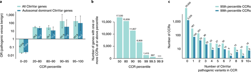
a, OR enrichment for ClinVar pathogenic variants versus benign variants for different CCR percentile bins among all autosomal ClinVar genes (light cyan) and genes that underlie autosomal dominant diseases (dark cyan). For all ClinVar genes, the error bars represent 95% CIs of 0.015–0.023 for the 0–20 percentile bin, 23.9–36.6 for the 20–80 percentile bin, 14.6–45.4 for the 80–90 percentile bin, 22.8–1,151.0 for the 90–95 percentile bin, and 40.4–647.5 for the 95–100 percentile bin. For autosomal dominant ClinVar genes, the 95% CIs are 0.017–0.035 for the 0–20 percentile bin, 14.3–34.3 for the 20–80 percentile bin, 5.12–25.7 for the 80–90 percentile bin, 5.32–269.5 for the 90–95 percentile bin, and 12.1–613.9 for the 95–100 percentile bin. A total of 24,554 pathogenic variants and 4,689 benign variants from ClinVar were intersected with CCRs; 10,781 pathogenic and 865 benign ClinVar variants lie within autosomal dominant genes. b, Histogram of the number of autosomal genes with at least one CCR greater than or equal to different percentile thresholds. c, Histogram of the number of 95th and 99th percentile CCRs with 0 to 10 or more overlapping ClinVar pathogenic variants. Highly constrained CCRs that harbor no known pathogenic variants may reflect regions under extreme purifying selection. Of the 24,554 ClinVar pathogenic variants, 2,172 (8.8%) and 551 (2.7%) were found in CCRs at or above the 95th and 99th percentile, respectively.

The most constrained CCRs are restricted to a small fraction of genes. Of the 17,693 Ensembl¹⁷ genes in the CCR model, only 39.0% and 8.0% of genes have at least one CCR in the 95th and 99th percentile or higher, respectively (Fig. 2b). Genes exhibiting multiple highly constrained regions (that is, ≥99th percentile) include many known to be involved in developmental delay, seizure disorders, and congenital heart defects, including KCNQ2, KCNQ5, SCN1A, SCN5A, multiple calcium voltage-gated channel subunits (for example, CACNA1A, CACNA1B, and CACNA1C), and GRIN2A (Supplementary Table 1). In addition, nine chromodomain helicase DNA-binding genes and the actin-dependent chromatin regulator subunits SMARCA2, SMARCA4, and SMARCA5 contain multiple 99th percentile CCRs. Such constraint likely reflects their role in chromatin remodeling, development, and severe disorders^18,19.

Finally, while highly constrained regions often contain one or more known pathogenic variants, 20,656 CCRs in the 95th percentile and 2,226 CCRs in the 99th percentile do not overlap a known pathogenic variant in ClinVar (Fig. 2c). We hypothesize that many of these regions are under extreme purifying selection, thus preventing the observation of a pathogenic variant among individuals studied to date. There is support for this hypothesis. Genes predicted to be essential, despite not having a known disease association²⁰, are significantly enriched relative to non-essential genes in the set of genes with at least one 95th percentile CCR (6,909 genes; one-tailed Fisher’s exact test, P = 2.8 × 10⁻¹⁰¹, OR = 3.24) or at least one 99th percentile CCR (1,415 genes; one-tailed Fisher’s exact test, P = 8.6 × 10⁻⁶⁷, OR = 3.73). Furthermore, genes in loci exhibiting low haplotype diversity are enriched for essential function^21,22 and are similarly prevalent among genes that have a 95th or 99th percentile CCR. This enrichment is significant (one-tailed Fisher’s exact test, P = 1.2 × 10⁻¹⁰ and OR = 4.0 for genes with 95th percentile CCR, P = 5.6 × 10⁻⁵ and OR = 4.4 for genes with 99th percentile CCR) compared with genes with higher haplotype diversity. Finally, Lelieveld et al.²³ recently reported 14 autosomal genes with focused clusters of de novo mutations from patients with intellectual disability and developmental disorders. The mutation clusters in 13 out of 14 of these genes coincide with a 95th percentile or higher CCR. The fact that these mutation clusters are typically no larger than 10 bp demonstrates that the most highly constrained CCRs reveal focal constraint. Taken together, these findings suggest that genes lacking a disease association, yet harboring one or more highly constrained CCRs, are under strong purifying selection owing to extreme fitness consequences when mutated.

Comparing intraspecies and interspecies constraint.

Given that most human genes are conserved among vertebrates, it is logical to expect that intraspecies constraint would be correlated with interspecies conservation, and that the most constrained CCRs would lie within conserved protein domains. To explore the relationship between intraspecies constraint and interspecies conservation, we compared CCRs to mammalian conservation measured by GERP++ (ref. ²⁴; Fig. 3a). As has been previously demonstrated^5,25, coding constraint is weakly correlated (Pearson r = 0.002 overall, r = 0.22 for CCRs above the 0th percentile) with conservation, illustrating that intraspecies constraint complements, and is not merely a subset of, interspecies conservation. As expected, 98.2% of the CCRs at the 95th percentile and above have mean GERP++ scores that suggest potential conservation in vertebrates (that is, >0.7 mean GERP++ score). However, 399 CCRs in 360 distinct genes are weakly conserved and suggest that some of these regions may represent recent constraint within the primate or human lineage (Fig. 3a, dotted box). For example, CDKN1C contains a 98.3 percentile CCR that coincides with a ClinVar variant known to be pathogenic for Beckwith–Wiedemann syndrome^26,27. CDKN1C is imprinted with preferential expression of the maternal allele²⁸, suggesting that monoallelic expression may, in part, underlie the degree of observed constraint as the expression of only one allele opens greater risk for a dominant phenotype. Furthermore, our model includes 30 of the 42 imprinted genes reported by Baran et al.²⁹ using data from the Genotype-Tissue Expression (GTEx) project. Of 30 imprinted genes, 16 (53%) harbor at least one CCR in the 95th percentile or higher: GRB10, IGF2, KCNQ1, KIF25, MAGEL2, MAGI2, MEST, NAP1L5, NTM, PEG10, PEG3, PLAGL1, SNRPN, SYCE1, UBE3A, and ZDBF2. This reflects a 1.35-fold enrichment over the 39% (6,909 of 17,693) of all genes in the CCR model having a CCR in at least the 95th percentile. Other genes harboring similarly dichotomous constraint and conservation measures include four members of the Fanconi anemia pathway (FAN1, SLX4, BOD1L1, and ERCC5), as well as an overrepresentation (P = 7.9 × 10⁻⁶; see Online Methods) of genes involved in the complement cascade of the innate immune system (Supplementary Table 2).

Fig. 3. The relationship between CCRs and interspecies conservation.

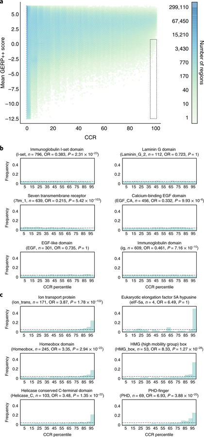
a, A comparison of intraspecies constraint (CCRs) and interspecies conservation, as measured by the mean GERP++ score in each CCR. Regions in the dotted box reflect intraspecies constraint not revealed by interspecies conservation. That is, they have a GERP++ score less than 0.7 and 95th percentile or greater CCR score. b, Example Pfam domain families for which constraint is nearly uniformly distributed among instances of the domain. c, Representative Pfam domain families exhibiting enrichment for higher levels of intraspecies constraint across the whole exome. P values and ORs reflect a Fisher’s exact test for a domain’s genomic intersection enrichment with CCRs in the 95th percentile or higher.

Motivated by prior analyses²⁵, we then explored the landscape of constraint in Pfam³⁰ domains, given that protein domains are conserved owing to their structural or functional role in proteins (Supplementary Dataset 1 and Supplementary Table 3). While we find constraint to typically be uniformly distributed over many protein domains (Fig. 3b), several families are enriched for high constraint, likely owing to their critical function in proteins that contain them (Fig. 3c). Constraint within ion transport domains is expected given their role in regulating the critical specificity of ion transport and the fact that mutations in these domains cause autosomal dominant encephalopathies³¹, neuropathies³², and cardiomyopathies³³. Furthermore, homeobox domains bind DNA and are involved in cellular differentiation and maintaining pluripotency³⁴. Helicase superfamily C-terminal domains catalyze DNA unwinding and are implicated in α-thalassemia³⁵ and intellectual disability³⁶. Moreover, PHD finger domains are found in many chromatin remodeling proteins, which, when perturbed, lead to various disorders^37–39. Finally, the eIF-5a domain is solely found in the two EIF5A translation initiation factors. These are the only human proteins that utilize the rare amino acid hypusine. Strikingly, a 99.47 percentile CCR coincides with the hypusine residue in the primary isoform of EIF5A. Knockout of either the EIF5A gene or the deoxyhypusine synthase gene, whose product is necessary to create the hypusine amino acid for EIF5A, causes embryonic lethality in mice⁴⁰.

It is notable that 34.2% (7,397 of 21,650) and 22.5% (554 of 2,465) of 95th and 99th percentile CCRs, respectively, do not coincide with an annotated Pfam domain. While CCRs that are proximal to annotated Pfam domains likely reflect truncated annotations caused by reduced homology or the consequence of homology searches driven by local alignment, distal CCRs may represent coding regions of previously uncharacterized functional or structural properties of the messenger RNA or protein.

Comparing CCRs to other models of constraint.

Although gene-wide metrics such as pLI cannot capture regional variability in constraint, genic intolerance to loss-of-function variation is often driven by focal constraint within critical regions of the gene. Therefore, as expected, autosomal genes with multiple CCRs above the 95th percentile are moderately correlated (Pearson r = 0.47) with high pLI values (Fig. 4a), as well as with gene-wide constraint measured by the missense Z⁵ and RVIS² statistics (Supplementary Fig. 4). Nonetheless, the CCR model reveals focal constraint missed by gene-wide measures (for example, Fig. 1b), as many genes with pLI probabilities close to 0 contain CCRs above the 95th percentile, illustrating the increased resolution of a regional constraint model.

Fig. 4. A comparison of CCRs with other models of genic and regional constraint.

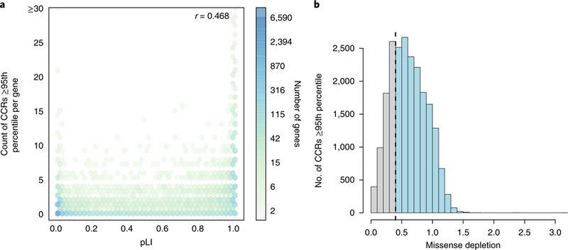
a, The correlation (Pearson r) between a gene’s pLI and the number of CCRs in the 95th percentile or higher observed in the gene. In general, genes with high pLI (>0.9) tend to harbor many such CCRs, while genes with low pLI (<0.1) do not. However, many low-pLI genes exhibit focal constraint at or above the 95th percentile. b, The relationship between CCRs in the 95th percentile or higher and the missense depletion score for the same coding region. The dashed line reflects the missense depletion threshold (ɣ > 0.4) below which Samocha et al.⁴¹ define regional constraint. Light blue bars beyond this threshold reflect CCRs at or above the 95th percentile that would not be deemed as constrained by the missense depletion metric. Gray bars reflect CCRs that coincide with regions deemed to be under constraint by missense depletion. There are 8,065,333 unique CCRs, with 21,650 at or above the 95th percentile.

In an effort to move beyond gene-wide constraint models, Samocha et al.⁴¹ recently described an approach to identify regions of protein-coding genes that exhibit ‘missense depletion’: that is, regions where far less than expected missense variation is observed in the Exome Aggregation Consortium (ExAC) v.1 catalog of 60,706 exomes. While the motivation is similar to our model of regional constraint, the missense depletion approach partitions solely 15.1% of transcripts into distinct missense depletion regions. That is, for 85% of transcripts, the entire transcript is assigned a single, summary constraint measure, and only 5.1% of transcripts are partitioned into three or more distinct regions of missense depletion. The missense depletion approach also chooses a single representative transcript for each gene; thus, coding exons exclusive to other isoforms are not modeled. Since CCRs measure constraint variability along the entire gene, they provide a more detailed map of the spectrum of constraint and identify areas of high constraint that would otherwise be missed. As a result, of the top 5% most constrained CCRs, 15,874 would be classified as either ‘unconstrained’ or ‘moderately constrained’ by the missense depletion threshold (ɣ > 0.4) (Fig. 4b), and 1,091 of the top 1% CCRs would be similarly missed. These CCRs lie within 5,981 and 802 distinct genes, respectively, and many have known associations with autosomal dominant disease (Supplementary Table 4). Furthermore, 3,707 unique genes containing a 95th percentile CCR are not predicted to be constrained by either pLI or the missense depletion statistic (Supplementary Fig. 5). Therefore, the CCR model complements the constraint predictions made by both gene-wide and regional constraint metrics, especially since CCRs specify a detailed constraint architecture for 88% of the autosomal exome, whereas the missense depletion metric coarsely delineates regional constraint for 15% of the protein coding transcripts.

Using CCRs to assist in the interpretation of de novo mutations in disease studies.

Since the most highly constrained CCRs are, by definition, devoid of protein-changing variants observed even as a heterozygote in a single individual from gnomAD, we should expect true regions of high constraint to often coincide with pathogenic mutations observed in patients with de novo dominant disorders. We tested this hypothesis by comparing the enrichment of 5,113 de novo missense mutations (DNMs) in 5,620 neurodevelopmental disorder probands^42–47 (‘pathogenic’ mutations) versus 1,269 DNMs from 2,078 unaffected siblings of autism spectrum disorder probands (‘benign’ mutations)^48,49 (see Supplementary Table 8 from ref. ⁴¹). This analysis results in a 7.1-fold enrichment of pathogenic DNMs from neurodevelopmental disorder cases in the most constrained (that is, at or above the 95th percentile) CCRs, and a 4.0-fold depletion of pathogenic DNMs in the least constrained CCRs (Fig. 5a). We then compared the ability of CCRs to evaluate these sets of pathogenic and benign mutations with that of GERP++, CADD⁵⁰, REVEL⁵¹, pLI⁴, MPC⁴¹, and MTR⁵². Although the performance of all methods is modest, CCRs yield the highest receiver operating characteristic (ROC) area under the curve (AUC) among tested methods (0.73; Fig. 5b and precision-recall analysis in Supplementary Fig. 6)⁵³. A complementary analysis of the X chromosome CCR model demonstrates similar performance (Supplementary Fig. 7).

Fig. 5. Evaluation of de novo mutations from a cohort with severe developmental delay, intellectual disability, and epileptic encephalopathy versus de novo variation from unaffected siblings of autism probands.

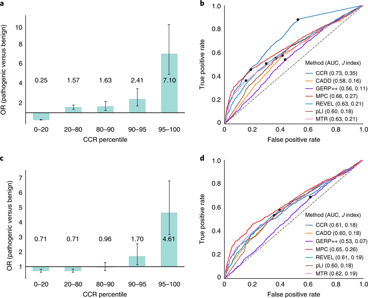
a, Enrichment of pathogenic de novo mutations in the most constrained CCRs, excluding pathogenic variants present in gnomAD. The 95% CI error bars are 0.22–0.29 for the 0–20 percentile bin, 1.36–1.81 for the 20–80 percentile bin, 1.24–2.16 for the 80–90 percentile bin, 1.66–3.50 for the 90–95 percentile bin, and 4.96–10.2 for the 95–100 percentile bin. b, ROC analysis for the developmental disorder de novo variant evaluation set described for a, where true positives are the pathogenic mutations and true negatives are the set of benign mutations. Of the 3,400 pathogenic and 1,269 benign mutations, each tool scored (M pathogenic; N benign): CCR (3,108; 1,149), CADD (3,399; 1,269), GERP++ (3,400; 1,269), MPC (3,221; 1,205), REVEL (3,368; 1,251), pLI (3,283; 1,212), MTR (3,389; 1,260). The dots in b and d indicate the score cutoff with the maximal Youden J statistic for each tool. Values in parenthesis indicate the AUC and the maximal J, respectively. c, Enrichment of pathogenic de novo mutations in the most constrained CCRs, after excluding benign and pathogenic mutations on the basis of their presence in gnomAD. The 95% CI error bars are 0.59–0.85 for the 0–20 percentile bin, 0.60–0.84 for the 20–80 percentile bin, 0.72–1.28 for the 80–90 percentile bin, 1.13–2.56 for the 90–95 percentile bin, and 3.16–6.81 for the 95–100 percentile bin. d, ROC analysis for the developmental disorder de novo variant evaluation set from c. Of the 3,400 pathogenic and 731 benign mutations, each tool scored (M pathogenic; N benign): CCR (3,108; 670), CADD (3,399; 731), GERP++ (3,400; 731), MPC (3,221; 704), REVEL (3,368; 726), pLI (3,283; 709), MTR (3,389; 728). CIs for each metric’s ROC AUC in b: CCR (0.711–0.745), CADD (0.567–0.603), GERP++ (0.542–0.579), MPC (0.643–0.676), REVEL (0.612–0.646), pLI (0.586–0.622), MTR (0.608–0.642). CIs for the ROC AUCs in d: CCR (0.586–0.629), CADD (0.581–0.624), GERP++ (0.509–0.556), MPC 0.627–0.667), REVEL (0.593–0.635), pLI (0.576–0.621), MTR (0.598–0.639).

Since the boundaries of constrained regions are defined by gnomAD variants, and more than one-third of de novo mutations have been observed as standing variation⁵⁴, we repeated these analyses while excluding any benign or pathogenic mutation present in gnomAD. While reduced, the enrichment (OR = 4.61) of pathogenic DNMs remains statistically significant at the 95th percentile (Fig. 5c). Furthermore, given the prevalence of recurrently mutating loci⁴ in the human genome, it is commonplace^46,55–57 to not exclude de novo mutations based upon their presence in reference databases. We therefore anticipate that the enrichment observed at the 95th percentile in Fig. 5a is indicative of future analyses. However, given the comparable performance of CCRs to other metrics (Fig. 5b,d), we emphasize that CCRs are insufficient as a standalone metric for prioritizing de novo mutations. For example, while a mutation coinciding with a high-percentile CCR is compelling support for its pathogenicity, the inverse is not necessarily true. Lying within a low-percentile CCR does not strictly imply that the mutation is benign. Therefore, in the context of rare disease research, we recommend the use of high-percentile CCRs as an annotation to complement the predictions made by variant prioritization tools.

Estimating the rate of false positive discovery of coding constraint.

The explosive human population growth over the last two millennia⁵⁸ and the resulting excess of very rare genetic variation in the human genome raise a natural question about our model of coding constraint: is constraint measured from 123,136 exomes sufficient to empower the prioritization of mutations in newly sequenced disease cohorts? Zou et al.⁵⁹ estimate that even 500,000 individuals will be insufficient to catalog the majority of protein-changing variants in the human population. Yet if predicted regions of constraint are truly under strong purifying selection, they should remain largely free of protein-changing variation, even as genetic variation is collected from much larger cohorts mostly composed of healthy individuals.

To test the predictive power of the current model, we compared CCRs to DNMs observed in both the neurodevelopmental disorder probands and the unaffected siblings of autism probands. As above, we assumed that DNMs from neurodevelopmental disorder probands represent true positives. DNMs from unaffected siblings represent true negatives, and thus false positives when they lie in regions of highest constraint. We measured the false discovery rate (FDR) of each CCR in the 90th, 95th, and 99th percentiles (Table 1 and Methods). We estimate an FDR of 2.8% from the fraction of CCRs in the 99th percentile and higher that coincide with a DNM from an unaffected sibling. Merely 0.6% of these ostensibly benign DNMs lie within a 99th percentile or higher CCR. This suggests that, while many more genomes are necessary to identify all variation in the human genome, our model illuminates coding regions under true constraint at a low predicted FDR.

Table 1 |.

Estimated FDR and false positive rate for the 90th, 95th, and 99th percentiles

Minimum CCR percentile	FDR	False positive rate
90	0.077	0.057
95	0.055	0.029
99	0.028	0.006

A total of 3,400 DNMs from neurodevelopmental disorder probands are treated as true positives; 1,269 DNMs from unaffected siblings of autism probands represent true negatives, and when overlapping a CCR, they are treated as false positives. FDR is calculated as false positives/(false positives + true positives) and false positive rate as false positives/(false positives + true negatives).

A fundamental strength of our approach is that the resolution of predicted constraint can, in principle, improve as variation from larger cohorts of individuals free of developmental disorders is sequenced. To test the expected increase in the resolution of coding constraint with larger sample sizes, we compared the described CCR model created from 123,136 gnomAD individuals to a CCR model based on the 60,706 individuals in ExAC v.1. As expected, we find that the enrichment of known ClinVar pathogenic mutations at the 95th percentile in the gnomAD model (OR = 161.8) is significantly greater than the enrichment observed for the ExAC v.1 CCR model (OR = 22.8; Supplementary Fig. 8).

Discussion

Deep sampling of human variation provides a richly textured ‘topographical map’ of constraint within protein-coding genes. The map of CCRs we have created highlights the largest voids of protein-changing variation from a sample of 246,272 human chromosomes. We hypothesize that such regions are depleted for protein-changing variation because mutations therein have strong selective pressures against them. Supporting this hypothesis, we have shown that CCRs at or above the 95th percentile are enriched for disease-causing variants, especially in dominant Mendelian disorders. Furthermore, protein domains with critical function are enriched for the highest local constraint. These observations demonstrate the utility of CCRs for prioritizing de novo mutations and rare variants in studies of dominant disease phenotypes. While correlated, local coding constraint complements phylogenetic conservation measures. The work of Samocha et al.⁴¹ suggests that future improvements in variant prioritization will arise by combining models of local coding constraint with single-nucleotide metrics that incorporate complementary information such as phylogenetic conservation, amino acid substitution scores, and three-dimensional protein structure.

Although we have demonstrated that highly constrained CCRs recover variants known to underlie human disease, we acknowledge that our approach is conservative. By requiring the complete absence of protein-changing variation within a CCR, we are prone to false negatives in larger constrained regions where variation is extremely sparse yet not completely absent in healthy individuals. This problem is likely to worsen with variant sets from ever larger cohorts, given that pathogenic variants with reduced penetrance are more likely to be included. We argue, however, that this complication reduces sensitivity for detecting constraint rather than creating spurious constraint predictions. Indeed, the precisely resolved regions that remain in light of such variants will represent even more confident predictions of regional constraint that are intolerant of any variation. We also emphasize that the presented approach is a simplification of a more general strategy that defines constrained regions based upon flanking variants meeting a minimum allele or genotype frequency. We anticipate that such extensions to our approach could be used to mitigate the effect of ‘contamination’ from recessive or incompletely penetrant alleles in future models. This will be the focus of future research as new population-scale variant catalogs emerge.

Nonetheless, our current method provides higher resolution than existing gene-wide constraint measures and minimizes false positives by strictly identifying regions with the highest constraint within each gene. CCRs are ill-suited to recessive disease yet empowered to reveal constrained regions under autosomal dominant disease models. Therefore, CCRs are best suited to the interpretation of de novo mutations observed in rare disease cohorts. Another important caveat of our model is that 55% (76,266 of 138,632) of the individuals sequenced in the gnomAD cohort are of European ancestry. As a result, the local coding constraint we predict has lesser predictive power for mutations observed in non-European individuals. However, we expect that the majority of truly constrained regions in any one population will also be constrained in others.

Looking forward, we argue that the most useful outcome of detailed maps of coding constraint is the ability to highlight critical regions in genes that have not yet been linked to human disease phenotypes. We have shown that the most constrained regions are enriched for disease-causing variants (Fig. 1a). However, more than 72% of genes harboring at least one CCR in the 99th percentile or higher lack any known pathogenic or likely pathogenic variants in ClinVar. It is likely that some of these regions exhibit such extreme constraint because mutations therein either lead to extreme developmental disorders or are embryonic lethal. Investigating the phenotypic effects of disrupting these regions provides an opportunity to identify new coding regions that drive disease phenotypes and are vital to human fitness.

Methods

CCR model construction.

The map of CCRs is constructed from the catalog of genetic variation observed among 123,136 exomes in gnomAD (https://storage.googleapis.com/gnomad-public/release/2.0.1/vcf/exomes/gnomad.exomes.r2.0.1.sites.vcf.gz). We first applied vt⁶¹ variant normalization and decomposition to the gnomAD VCF using the commands ‘vt decompose $gnomad_vcf -o $gnomad_ decomp_vcf -s’ and ‘vt normalize $gnomad_decomp_vcf -o $gnomad_decomp_ norm_vcf -r grch37.fasta’.

We then annotated the decomposed and normalized gnomAD VCF file with VEP⁶² (v.81 using Ensembl v.75 transcripts). The CCR model uses solely variants that VEP predicts to be ‘protein-changing’, which we define as any variant having the following Sequence Ontology terms for at least one Ensembl transcript: ‘missense_variant’, ‘stop_gained’, ‘stop_lost’, ‘start_lost’, ‘frameshift_variant’, ‘initiator_codon_variant’, ‘rare_amino_acid_variant’, ‘protein_altering_variant’, ‘inframe_insertion’, ‘inframe_deletion’, and ‘splice_donor_variant’ or ‘splice_ acceptor_variant’ when paired with ‘coding_sequence_variant’. In addition, the variants must have a filter value of ‘PASS’, ‘SEGDUP’, or ‘LCR’. The rationale behind including ‘LCR’ and ‘SEGDUP’ labeled variants is that we already account for segmental duplications and self-chains in our model.

Coding exons from all protein-coding transcripts in ENSEMBL¹⁷ v.75 were ‘flattened’ into a single, combined model of coding sequence for each gene. Constraint ‘regions’ are defined by measuring the exonic nucleotide distance between each pair of protein-changing variants, excluding the 5ʹ and 3ʹ variants flanking each region, as the flanking variants are inferred to represent the least constraint. We did not impose a minimum distance between protein-changing variants. Constraint regions can encompass a single exon or span multiple exons.

To prevent false identification of constraint that could arise solely because of reduced power to detect genetic variation, the length of each region is weighted by the fraction of individuals in gnomAD having at least 10× coverage at each bp. For example, if a region is 100 bp long and at each bp 90% of individuals have 10× coverage, the resulting weighted distance would be 90. Additionally, if the coverage for a single base falls below 50% of gnomAD individuals having at least 10× coverage, the region is immediately broken and a new region is not started until the coverage exceeds 50% of individuals at 10× coverage. Finally, coding regions that overlap either segmental duplications or self-chain alignments with at least 90% identity are removed from our model. The rationale is that we cannot trust variant patterns in these regions owing to known artifacts that may arise when aligning short sequencing reads to paralogous genome segments.

For all remaining constraint regions, we compute the region’s CpG density as a proxy for the region’s mutability owing to spontaneous deamination of methylated cytosines. We then create a linear regression of the weighted length (dependent variable) versus CpG density (independent variable) for all regions. Each region’s degree of constraint is measured on the basis of its distance from the resulting regression line. Regions having a greater weighted distance between protein-changing variants than expected based upon their CpG density (the residual from the linear regression line) are predicted to be under the greatest constraint. The resulting residuals are scaled from 0 to 100, ranked by residual (highest to lowest), and assigned a percentile such that regions with the largest residual value are assigned the highest percentile, reflecting the highest predicted constraint. Genomic positions harboring observed variants in gnomAD are assigned the lowest residual and a percentile of 0. This is based on the fact that such variants were obtained from individuals who either are healthy or did not have developmental abnormalities and should therefore be interpreted as unconstrained loci.

Lastly, since the gnomAD dataset contains ~25% fewer X chromosomes than autosomes, assuming a composition of males and females, constrained regions on the X chromosome are likely to be larger, on average, owing to less observed genetic variation. We therefore generated a separate model of constraint for the X chromosome that incorporates solely the coding gnomAD variants observed on the X chromosome. This X-specific model uses the same coverage cutoff and fraction of individuals as the full autosomal model, as well as the same source self-chains and segmental duplication exclusions.

Evaluation of CCRs with ClinVar.

ORs were used to test the power of our CCRs to predict the pathogenicity of new variants using ClinVar variants (v.20170802, ftp://ftp.ncbi.nih.gov/pub/clinvar/vcf_GRCh37/archive_2.0/2017/clinvar_20170802.vcf.gz) as a truth set. Our evaluation set consisted of solely ClinVar variants that were designated as ‘pathogenic’ or ‘likely pathogenic’ for true positive variants and ‘benign’ as true negative variants. All variants from both sets were also required to have at least ‘criteria provided, single submitter’ review status or greater with no conflicts. Any variant designated as ‘no assertion criteria provided’, ‘no assertion provided’, or ‘no interpretation for the single variant’ was excluded from the evaluation set. Variant alleles were also excluded if they matched those observed in ExAC v.1 and gnomAD datasets. True positive (pathogenic) and true negative (benign) variants were also required to have a predicted impact of ‘stop_gained’, ‘stop_lost’, ‘start_lost’, ‘initiator_codon’, ‘rare_amino_acid’, ‘missense’, ‘protein_ altering’, ‘frameshift’, ‘inframe_deletion’, ‘inframe_insertion’, or ‘coding_sequence_ variant’ combined with either ‘splice_acceptor_variant’ or ‘splice_donor_variant’. These restrictions resulted in 2,677 genes, 24,544 pathogenic and 4,689 benign variants from ClinVar when including all disease inheritance models. They resulted in 478 genes, 10,781 pathogenic, and 865 benign variants when including solely autosomal dominant disorders.

ORs in Fig. 2a were based on a curated set of genes underlying autosomal dominant disease phenotypes from Berg et al.⁶³. ORs for each percentile bin were calculated by $\text{OR}=\frac{a/b}{c/d}$, where a is the number of pathogenic variants in a bin, b is the number of benign variants in a bin, c is the number of pathogenic variants not in the bin, and d is the number of benign variants not in the bin. In other words, we are measuring the ratio of pathogenic variants in the bin to benign variants in that bin divided by the ratio of pathogenic variants not in that bin to the benign variants not in that bin. We also calculated 95% percent CIs from the standard error, $\text{s.e.}=\sqrt{\left(1/a\right)+\left(1/b\right)+\left(1/c\right)+\left(1/d\right)}$. The lower bound of the CI is calculated using the expression $e^{\text{ln}\left[OR\right]-1.96\times \text{s.e.}}$, and the upper bound of the CI is calculated by $e^{\text{ln}\left[OR\right]+1.96\times \text{s.e.}}$.

We report the values for each cell of the contingency table used for the Fisher’s exact test OR calculation in each percentile range below as follows [in percentile bin and pathogenic; not in percentile bin and pathogenic; in percentile bin and benign; not in percentile bin and benign]: All ClinVar genes: 0–20 bin, [11,468.0; 16,276.0; 3,855.0; 102.0]; 20–80 bin, [11,073.0; 16,671.0; 87.0; 3,870.0]; 80–90 bin, [2,014.0; 25,730.0; 12.0; 3,945.0]; 90–95 bin, [1,091.0; 26,653.0; 1.0; 3,956.0]; 95–100 bin, [2,098.0; 25,646.0; 2.0; 3,955.0]. Autosomal dominant ClinVar genes: 0–20 bin, [4,968.0; 8,137.0; 729.0; 29.0]; 20–80 bin, [5,074.0; 8,031.0; 21.0; 737.0]; 80–90 bin, [1,098.0; 12,007.0; 6.0; 752.0]; 90–95 bin, [624.0; 12,481.0; 1.0; 757.0]; 95–100 bin, [1,341.0; 11,764.0; 1.0; 757.0].

Evaluation of CCRs on neurodevelopmental disorder versus control de novo mutations.

We used OR comparisons to test the power of our CCRs to predict the pathogenicity of new variants that lie within their boundaries, and in this case, a well-curated set of DMNs was used as a truth set. The set of DNMs curated by Samocha et al.⁴¹ was used as an independent truth set for evaluating CCRs and other variant pathogenicity prediction tools. Predicted pathogenic variants in this truth set are composed of DNMs observed in individuals with developmental delay, severe intellectual disability, and epileptic encephalopathy^42–47. Predicted benign variants reflect DNMs from unaffected siblings of autism probands^48,49. Pathogenic mutations were filtered on their presence in ExAC v.1 and gnomAD. ORs and CIs were calculated as above.

We report the values for each cell of the contingency table used for the Fisher’s exact test OR calculation in each percentile range below as follows [in percentile bin and pathogenic; not in percentile bin and pathogenic; in percentile bin and benign; not in percentile bin and benign]: Fig. 5a: 0–20 bin, [757.0; 2,388.0; 648.0; 508.0]; 20–80 bin, [1,358.0; 1,787.0; 377.0; 779.0]; 80–90 bin, [279.0; 2,866.0; 65.0; 1,091.0]; 90–95 bin, [208.0; 2,937.0; 33.0; 1,123.0]; 95–100 bin, [543.0; 2,602.0; 33.0; 1,123.0]. Figure 5c: 0–20 bin, [757.0; 2,388.0; 208.0; 466.0]; 20–80 bin, [1,358.0; 1,787.0; 348.0; 326.0]; 80–90 bin, [279.0; 2,866.0; 62.0; 612.0]; 90–95 bin, [208.0; 2,937.0; 27.0; 647.0]; 95–100 bin, [543.0; 2,602.0; 29.0; 645.0]. Supplementary Fig 7a (X chromosome CCRs): 0–20 bin, [17.0; 138.0; 20.0; 16.0]; 20–80 bin, [55.0; 100.0; 13.0; 23.0]; 80–90 bin, [28.0; 127.0; 2.0; 34.0]; 90–95 bin, [20.0; 135.0; 0.0; 36.0]; 95–100 bin, [35.0; 120.0; 1.0; 35.0].

Comparing CCRs to missense depletion scores.

We compared CCRs in the 99th percentile and higher to missense depletion scores defined by Samocha et al.⁴¹ by intersecting CCR regions with missense depletion regions using bedtools⁶⁴. CCRs to the right of the black dashed vertical line in Fig. 4b reflect highly constrained CCRs that fall below the threshold (0.4) for significant missense depletion defined by Samocha et al.

CCRs in Pfam domain families.

Human genome build 37 genome coordinates for Pfam domains were curated from the University of California, Santa Cruz (UCSC) Table Browser (Pfam Domains in UCSC Genes track). Pfam domain families were then intersected with all CCRs to measure the distribution of regional constraint across each protein domain family. Under a null hypothesis of a uniform distribution of CCRs overlapping domains across different percentiles, we used a two-tailed Fisher’s exact test to ask whether there is an enrichment of domain intersections with CCRs in the 95th percentile or higher. For each Pfam domain, a contingency table was constructed with the following cells: (1) the count of unique CCRs at the 95th percentile or higher that intersected the given Pfam domain, (2) the count of all unique CCRs below the 95th percentile that intersected the given Pfam domain, (3) the count of all CCRs at or above the 95th percentile that intersect with other Pfam domains, and (4) the count of all CCRs below the 95th percentile that intersect with other Pfam domains. The OR is calculated as $\text{OR}=\frac{a/b}{c/d}$. P value is calculated as $P=\frac{\left(a+b\right)!\left(c+d\right)!\left(a+c\right)!\left(b+d\right)!}{a!b!c!d!n!}$. The internal control for the inherently greater length of the 95th percentile and higher CCRs comes from the fact that these CCRs are not only intersected with the Pfam domain intervals of interest (a in the above calculation) but also with all other Pfam domain intervals as a control (c in the above calculation). This gives these CCRs equal opportunity to overlap not only with the Pfam domain in question but also with all other Pfam domains. The Fisher’s exact test is therefore testing for the enrichment of ≥95th percentile CCRs with the Pfam domain of interest versus the enrichment of these CCRs with all other Pfam domains. Furthermore, it also tests for similar enrichment in CCRs below the 95th percentile (b and d in the above calculation). We emphasize that we use the count of intersections in this test rather than the number of bp, because the Fisher’s exact test assumes that every intersection is independent. However, since bp from the same CCR are clearly not independent, we use the count of intersections for each cell of the contingency table.

Comparing vertebrate conservation to regional coding constraint.

To evaluate the enrichment of highly constrained CCRs in Pfam domains, we divided CCR percentiles into 20 equal ranges (for example, 0–5%, 5–10%, …, 95–100%) and measured the proportion of Pfam domain bp intersecting each CCR percentile range. We then used a binomial test (expected success rate = 0.05) to assess the significance of enrichment in the highest CCR bin (95% or greater). The number of overlapping bases across all CCRs was used as the number of trials. We investigated the relationship between CCR percentiles and vertebrate conservation scores by intersecting CCRs with per-base GERP++ scores. The mean GERP++ score was calculated for each CCR. We defined CCRs in the 95th percentile or higher as constrained yet not conserved if the CCR had a mean GERP++ rejected substitution score of less than 0.7 RS, as this falls 1 RS below the GERP++ confidence threshold for interspecies mammalian constraint²⁴.

Comparing CCRs to other metrics for variant prioritization.

To understand how CCRs compare to other methods of variant pathogenicity prediction, we conducted a ROC curve analysis on the ClinVar truth set and a well-curated set of de novo variants in developmental disorders (described above). The true positives were taken from both the neurodevelopmental de novo and ClinVar pathogenic and likely pathogenic variant sets, respectively, filtered on matching ExAC v.1 and gnomAD alleles, and the true negatives are represented by the unaffected autism sibling de novo mutations and the ClinVar variants designated as benign.

We chose five metrics with which to compare CCRs. The first, MPC⁴¹, was chosen because it is the only other variant pathogenicity prediction tool that models regional constraint. Second, we chose REVEL⁵¹ because it is a recently developed tool that performs extremely well on ClinVar compared with all other metrics. Third, we chose GERP++ (ref. ²⁴) as a measure of conservation for a point of comparison between constraint and conservation in human-based pathogenicity prediction. Fourth, we chose CADD⁵⁰ as it is a widely used variant pathogenicity prediction method. Finally, MTR⁵² is a new, per-base metric that leverages a 93 bp sliding window to estimate local constraint.

ROC curves were calculated using scikit-learn in Python 2.7. We included solely variants defined as protein-changing by pathoscore (https://github.com/quinlan-lab/pathoscore), as explained above in the section ‘Evaluation of CCRs with ClinVar’. CIs for the AUC of each metric were calculated with the pROC R package (https://cran.r-project.org/web/packages/pROC/).

Gene pathway and subnetwork over-representation analysis.

We used the ‘pathway-based sets’ gene set over-representation method from ConsensusPathDB (http://cpdb.molgen.mpg.de/) to test for gene over-representation in distinct pathways. The ConsensusPathDB over-representation is calculated using a binomial test, where the null hypothesis assumes that genes in the list given are sampled from the same superset and thus the probability of observing a gene in a pathway in the given list is the same as in the original superset⁶⁵.

Estimation of FDR and false positive rate.

We estimate FDR as false positives/(false positives + true positives), where true positives are the developmental de novos that lie within a CCR above our threshold, and false positives are the unaffected autism sibling de novos also above that threshold. Similarly, to estimate the false positive rate, we create an estimate using the equation false positive rate = false positives/(false positives + true negatives). We assume that, as with the FDR, the false positives are the true negatives above the CCR percentile cutoff, and that the true negatives are the set of all true negatives, which, in this case is a superset of the false positives. Therefore, the false positive rate is the true negatives above the cutoff divided by the number of all true negatives.

Correlating exonic CpG density with gnomAD variant density.

By employing the ‘flattened’ exons we utilized for the CCR model and by filtering out exon regions with the same restrictions (no coverage below of 50% at 10×, overlapping of segmental duplications or 90% identity self-chains), we calculated the CpG density of all exons that were at least 20 bp in length. Exonic CpG density was compared to the density of variant changes that were either ‘PASS,’ ‘SEGDUP,’ ‘LCR,’ or ‘RF’. We measured variant density of all variant types, as well as solely for C>T or G>A transitions that could be the result of deamination of a 5mC (5-methylcytosine).

Coverage threshold for optimization and creation of the model.

To justify our cutoff of 50% of individuals having coverage at 10×, and the use of 10× instead of another coverage cutoff, we created both ROC and precision-recall curves for various cutoffs of our model. We used 1× with a cutoff of 10%, 1× with a cutoff of 90%, 5× with a cutoff of 10%, 5× with a cutoff of 90%, 10× with a cutoff of 50%, 3× with a cutoff of 50%, 50× with a cutoff of 10%, and 50× with a cutoff of 90%. We chose a minimum of 10× coverage in 50% of gnomAD individuals since it performed as well as more restrictive thresholds (Supplementary Fig. 1). The model parameters besides coverage were the same for all instances of the model used in the comparison.

Comparing CCR models created from variation observed in larger cohorts.

As a demonstration of the improvement in granularity in our model when more individuals are sequenced for variants, we compared our CCR model based on gnomAD (ExAC v.2) with 123,136 individuals to an older version based on ExAC v.1 containing 60,706 individuals’ variant data. The OR comparison was performed for percentile bins 0–20, 20–80, 80–90, 90–95, and 95–100 as with the gnomAD version in Figs. 2 and 5.

We report the values for each cell of the contingency table used for the Fisher’s exact test OR calculation in each percentile range below as follows [in percentile bin and pathogenic; not in percentile bin and pathogenic; in percentile bin and benign; not in percentile bin and benign]: For the gnomAD version of CCR the numbers are the same as for Fig. 2a. For the ExAC v.1 version of CCR: 0–20 bin, [9,283.0; 17,042.0; 3,787.0; 169.0]; 20–80 bin, [11,400.0; 14,925.0; 119.0; 3,837.0]; 80–90 bin, [2,081.0; 24,244.0; 25.0; 3,931.0]; 90–95 bin, [1,202.0; 25,123.0; 8.0; 3,948.0]; 95–100 bin, [2,359.0; 23,966.0; 17.0; 3,939.0].

Comparison to the missense Z, RVIS, and pLI metrics.

We assessed the correlation between the missense Z, RVIS, and pLI gene-wide constraint metrics and CCRs at or above the 95th percentile by comparing the count of 95th percentile or higher CCRs per gene with the constraint metrics’ values for the gene.

For missense Z constraint, we used Supplementary Table 13 from ref. ⁴, which contained missense Z constraint scores for every gene. pLI was obtained from the Broad Institute’s website at ftp://ftp.broadinstitute.org/pub/ExAC_release/release1/manuscript_data/forweb_cleaned_exac_r03_march16_z_data_pLI.txt.gz as well as from ref. ⁴. Lastly, the version of RVIS used for this comparison was the most up-to-date version based on CCDS v.20 and gnomAD data at http://genic-intolerance.org/data/RVIS_Unpublished_ExACv2_March2017.txt.

References

- 1.Wallis WA The statistical research group, 1942–1945. J. Am. Stat. Assoc 75, 320–330 (1980). [Google Scholar]
- 2.Petrovski S, Wang Q, Heinzen EL, Allen AS & Goldstein DB Genic intolerance to functional variation and the interpretation of personal genomes. PLoS Genet 9, e1003709 (2013). [DOI] [PMC free article] [PubMed] [Google Scholar]
- 3.Fu W et al. Analysis of 6,515 exomes reveals the recent origin of most human protein-coding variants. Nature 493, 216–220 (2013). [DOI] [PMC free article] [PubMed] [Google Scholar]
- 4.Lek M et al. Analysis of protein-coding genetic variation in 60,706 humans. Nature 536, 285–291 (2016). [DOI] [PMC free article] [PubMed] [Google Scholar]
- 5.Samocha KE et al. A framework for the interpretation of de novo mutation in human disease. Nat. Genet 46, 944–950 (2014). [DOI] [PMC free article] [PubMed] [Google Scholar]
- 6.Finn RD et al. The Pfam protein families database: towards a more sustainable future. Nucleic Acids Res 44, D279–D285 (2016). [DOI] [PMC free article] [PubMed] [Google Scholar]
- 7.Letunic I, Doerks T & Bork P SMART 7: recent updates to the protein domain annotation resource. Nucleic Acids Res 40, D302–D305 (2012). [DOI] [PMC free article] [PubMed] [Google Scholar]
- 8.Tatusov RL et al. The COG database: an updated version includes eukaryotes. BMC Bioinformatics 4, 41 (2003). [DOI] [PMC free article] [PubMed] [Google Scholar]
- 9.Klimke W et al. The National Center For Biotechnology Information’s Protein Clusters Database. Nucleic Acids Res 37, D216–D223 (2009). [DOI] [PMC free article] [PubMed] [Google Scholar]
- 10.Haft DH, Selengut JD & White O The TIGRFAMs database of protein families. Nucleic Acids Res 31, 371–373 (2003). [DOI] [PMC free article] [PubMed] [Google Scholar]
- 11.Bailey JA et al. Recent segmental duplications in the human genome. Science 297, 1003–1007 (2002). [DOI] [PubMed] [Google Scholar]
- 12.Cabanski CR et al. BlackOPs: increasing confidence in variant detection through mappability filtering. Nucleic Acids Res 41, e178 (2013). [DOI] [PMC free article] [PubMed] [Google Scholar]
- 13.Lister R et al. Human DNA methylomes at base resolution show widespread epigenomic differences. Nature 462, 315–322 (2009). [DOI] [PMC free article] [PubMed] [Google Scholar]
- 14.Aggarwala V & Voight BF An expanded sequence context model broadly explains variability in polymorphism levels across the human genome. Nat. Genet 48, 349–355 (2016). [DOI] [PMC free article] [PubMed] [Google Scholar]
- 15.Mugal CF & Ellegren H Substitution rate variation at human CpG sites correlates with non-CpG divergence, methylation level and GC content. Genome Biol 12, R58 (2011). [DOI] [PMC free article] [PubMed] [Google Scholar]
- 16.Carlson J et al. Extremely rare variants reveal patterns of germline mutation rate heterogeneity in humans Preprint at bioRxiv 10.1101/108290 (2017). [DOI] [PMC free article] [PubMed]
- 17.Yates A et al. Ensembl 2016. Nucleic Acids Res 44, D710–D716 (2016). [DOI] [PMC free article] [PubMed] [Google Scholar]
- 18.Marfella CGA & Imbalzano AN The Chd family of chromatin remodelers. Mutat. Res 618, 30–40 (2007). [DOI] [PMC free article] [PubMed] [Google Scholar]
- 19.Van Houdt JKJ et al. Heterozygous missense mutations in SMARCA2 cause Nicolaides-Baraitser syndrome. Nat. Genet 44, 445–449 (2012). [DOI] [PubMed] [Google Scholar]
- 20.Spataro N, Rodríguez JA, Navarro A & Bosch E Properties of human disease genes and the role of genes linked to Mendelian disorders in complex disease aetiology. Hum. Mol. Genet 26, 489–500 (2017). [DOI] [PMC free article] [PubMed] [Google Scholar]
- 21.Gibson J, Tapper W, Ennis S & Collins A Exome-based linkage disequilibrium maps of individual genes: functional clustering and relationship to disease. Hum. Genet 132, 233–243 (2013). [DOI] [PubMed] [Google Scholar]
- 22.Collins A The genomic and functional characteristics of disease genes. Brief. Bioinform 16, 16–23 (2014). [DOI] [PubMed] [Google Scholar]
- 23.Lelieveld SH et al. Spatial clustering of de novo missense mutations identifies candidate neurodevelopmental disorder-associated genes. Am. J. Hum. Genet 101, 478–484 (2017). [DOI] [PMC free article] [PubMed] [Google Scholar]
- 24.Davydov EV et al. Identifying a high fraction of the human genome to be under selective constraint using GERP++. PLoS Comput. Biol 6, e1001025 (2010). [DOI] [PMC free article] [PubMed] [Google Scholar]
- 25.Gussow AB, Petrovski S, Wang Q, Allen AS & Goldstein DB The intolerance to functional genetic variation of protein domains predicts the localization of pathogenic mutations within genes. Genome Biol 17, 9 (2016). [DOI] [PMC free article] [PubMed] [Google Scholar]
- 26.Lee MP et al. Low frequency of p57KIP2 mutation in Beckwith-Wiedemann syndrome. Am. J. Hum. Genet 61, 304–309 (1997). [DOI] [PMC free article] [PubMed] [Google Scholar]
- 27.Romanelli V et al. CDKN1C (p57Kip)) analysis in Beckwith-Wiedemann syndrome (BWS) patients: genotype-phenotype correlations, novel mutations, and polymorphisms. Am. J. Med. Genet. A 152A, 1390–1397 (2010). [DOI] [PubMed] [Google Scholar]
- 28.Higashimoto K, Soejima H, Saito T, Okumura K & Mukai T Imprinting disruption of the CDKN1C/KCNQ1OT1 domain: the molecular mechanisms causing Beckwith-Wiedemann syndrome and cancer. Cytogenet. Genome Res 113, 306–312 (2006). [DOI] [PubMed] [Google Scholar]
- 29.Baran Y et al. The landscape of genomic imprinting across diverse adult human tissues. Genome Res 25, 927–936 (2015). [DOI] [PMC free article] [PubMed] [Google Scholar]
- 30.Finn RD et al. The Pfam protein families database. Nucleic Acids Res 38, D211–D222 (2010). [DOI] [PMC free article] [PubMed] [Google Scholar]
- 31.Weckhuysen S et al. KCNQ2 encephalopathy: emerging phenotype of a neonatal epileptic encephalopathy. Ann. Neurol 71, 15–25 (2012). [DOI] [PubMed] [Google Scholar]
- 32.Tinel N, Lauritzen I, Chouabe C, Lazdunski M & Borsotto M The KCNQ2 potassium channel: splice variants, functional and developmental expression. Brain localization and comparison with KCNQ3. FEBS Lett 438, 171–176 (1998). [DOI] [PubMed] [Google Scholar]
- 33.Ocorr K et al. KCNQ potassium channel mutations cause cardiac arrhythmias in Drosophila that mimic the effects of aging. Proc. Natl Acad. Sci. USA 104, 3943–3948 (2007). [DOI] [PMC free article] [PubMed] [Google Scholar]
- 34.Mark M, Rijli FM & Chambon P Homeobox genes in embryogenesis and pathogenesis. Pediatr. Res 42, 421–429 (1997). [DOI] [PubMed] [Google Scholar]
- 35.Stevenson RE in GeneReviews (eds Adam MP et al. ) (Univ. Washington, 1993–2018). [Google Scholar]
- 36.Higgs DR et al. Understanding α-globin gene regulation: aiming to improve the management of thalassemia. Ann. NY Acad. Sci 1054, 92–102 (2005). [DOI] [PubMed] [Google Scholar]
- 37.Baker LA, Allis CD & Wang GG PHD fingers in human diseases: disorders arising from misinterpreting epigenetic marks. Mutat. Res 647, 3–12 (2008). [DOI] [PMC free article] [PubMed] [Google Scholar]
- 38.Musselman CA & Kutateladze TG PHD fingers: epigenetic effectors and potential drug targets. Mol. Interv 9, 314–323 (2009). [DOI] [PMC free article] [PubMed] [Google Scholar]
- 39.Matthews AGW et al. RAG2 PHD finger couples histone H3 lysine 4 trimethylation with V(D)J recombination. Nature 450, 1106–1110 (2007). [DOI] [PMC free article] [PubMed] [Google Scholar]
- 40.Nishimura K, Lee SB, Park JH & Park MH Essential role of eIF5A-1 and deoxyhypusine synthase in mouse embryonic development. Amino Acids 42, 703–710 (2012). [DOI] [PMC free article] [PubMed] [Google Scholar]
- 41.Samocha KE et al. Regional missense constraint improves variant deleteriousness prediction Preprint at bioRxiv 10.1101/148353 (2017). [DOI]
- 42.de Ligt J et al. Diagnostic exome sequencing in persons with severe intellectual disability. N. Engl. J. Med 367, 1921–1929 (2012). [DOI] [PubMed] [Google Scholar]
- 43.Rauch A et al. Range of genetic mutations associated with severe non-syndromic sporadic intellectual disability: an exome sequencing study. Lancet 380, 1674–1682 (2012). [DOI] [PubMed] [Google Scholar]
- 44.Lelieveld SH et al. Meta-analysis of 2,104 trios provides support for 10 new genes for intellectual disability. Nat. Neurosci 19, 1194–1196 (2016). [DOI] [PubMed] [Google Scholar]
- 45.Deciphering Developmental Disorders Study. Large-scale discovery of novel genetic causes of developmental disorders. Nature 519, 223–228 (2015). [DOI] [PMC free article] [PubMed] [Google Scholar]
- 46.Deciphering Developmental Disorders Study. Prevalence and architecture of de novo mutations in developmental disorders. Nature 542, 433–438 (2017). [DOI] [PMC free article] [PubMed] [Google Scholar]
- 47.Epi4K Consortium. et al. De novo mutations in epileptic encephalopathies. Nature 501, 217–221 (2013). [DOI] [PMC free article] [PubMed] [Google Scholar]
- 48.Iossifov I et al. The contribution of de novo coding mutations to autism spectrum disorder. Nature 515, 216–221 (2014). [DOI] [PMC free article] [PubMed] [Google Scholar]
- 49.De Rubeis S et al. Synaptic, transcriptional and chromatin genes disrupted in autism. Nature 515, 209–215 (2014). [DOI] [PMC free article] [PubMed] [Google Scholar]
- 50.Kircher M et al. A general framework for estimating the relative pathogenicity of human genetic variants. Nat. Genet 46, 310–315 (2014). [DOI] [PMC free article] [PubMed] [Google Scholar]
- 51.Ioannidis NM et al. REVEL: an ensemble method for predicting the pathogenicity of rare missense variants. Am. J. Hum. Genet 99, 877–885 (2016). [DOI] [PMC free article] [PubMed] [Google Scholar]
- 52.Traynelis J et al. Optimizing genomic medicine in epilepsy through a gene-customized approach to missense variant interpretation. Genome Res 27, 1715–1729 (2017). [DOI] [PMC free article] [PubMed] [Google Scholar]
- 53.Youden WJ Index for rating diagnostic tests. Cancer 3, 32–35 (1950). [DOI] [PubMed] [Google Scholar]
- 54.Kosmicki JA et al. Refining the role of de novo protein-truncating variants in neurodevelopmental disorders by using population reference samples. Nat. Genet 49, 504–510 (2017). [DOI] [PMC free article] [PubMed] [Google Scholar]
- 55.Turner TN et al. Genomic patterns of de novo mutation in simplex autism. Cell 171, 710–722 (2017). [DOI] [PMC free article] [PubMed] [Google Scholar]
- 56.Werling DM et al. An analytical framework for whole-genome sequence association studies and its implications for autism spectrum disorder. Nat. Genet 50, 727–736 (2018). [DOI] [PMC free article] [PubMed] [Google Scholar]
- 57.Homsy J et al. De novo mutations in congenital heart disease with neurodevelopmental and other congenital anomalies. Science 350, 1262–1266 (2015). [DOI] [PMC free article] [PubMed] [Google Scholar]
- 58.Keinan A & Clark AG Recent explosive human population growth has resulted in an excess of rare genetic variants. Science 336, 740–743 (2012). [DOI] [PMC free article] [PubMed] [Google Scholar]
- 59.Zou J et al. Quantifying unobserved protein-coding variants in human populations provides a roadmap for large-scale sequencing projects. Nat. Commun 7, 13293 (2016). [DOI] [PMC free article] [PubMed] [Google Scholar]
- 60.Villard E et al. Mutation screening in dilated cardiomyopathy: prominent role of the beta myosin heavy chain gene. Eur. Heart J 26, 794–803 (2005). [DOI] [PubMed] [Google Scholar]
- 61.Tan A, Abecasis GR & Kang HM Unified representation of genetic variants. Bioinformatics 31, 2202–2204 (2015). [DOI] [PMC free article] [PubMed] [Google Scholar]
- 62.McLaren W et al. The Ensembl Variant Effect Predictor. Genome Biol 17, 122 (2016). [DOI] [PMC free article] [PubMed] [Google Scholar]
- 63.Berg JS et al. An informatics approach to analyzing the incidentalome. Genet. Med 15, 36–44 (2013). [DOI] [PMC free article] [PubMed] [Google Scholar]
- 64.Quinlan AR & Hall IM BEDTools: a flexible suite of utilities for comparing genomic features. Bioinformatics 26, 841–842 (2010). [DOI] [PMC free article] [PubMed] [Google Scholar]
- 65.Mi H, Muruganujan A, Casagrande JT & Thomas PD Large-scale gene function analysis with the PANTHER classification system. Nat. Protoc 8, 1551–1566 (2013). [DOI] [PMC free article] [PubMed] [Google Scholar]
Associated Data
This section collects any data citations, data availability statements, or supplementary materials included in this article.