On the Growth Rate of Spherulites and Axialites from the Melt in Polyethylene Fractions: Regime I and Regime II Crystallization

The growth rate G of the crystalline bodies appearing in each of a set of 35 characterized polyethylene fractions ranging from 3600 to 807,000 in molecular weight has been measured as a function of the undercooling ΔT. In isothermal crystallization, only axialites were found from M_w = 3600 to 18,000. (For these runs, ΔT < 17.5 °C.) From M_w = 18,000 to M_w ≅ 115,000 coarse-grained non-banded spherulites were found for ΔT > 17.5 °C, and axialites for ΔT < 17.5 °C; a rather sharp break occurred in the logio G versus T data at ΔT ≅ 17.5 °C. The morphologic al changes were more gradual. Above M_w = 115,-000, only nearly structureless “irregular” spherulites were found at all undercoolings corresponding to isothermal growth. Typical ringed spherulites were obtained only on quenching. Wide-angle x-ray data showed that the usual orthorhombic subcell predominated in all the morphologies encountered. Low-angle x-ray data showed that the specimens exhibited lamellar crystallization irrespective of the particular gross morphology involved. The growth rate data on each fraction were analyzed using

$$G=G_0\text{\hspace{0.17em}exp}\left[-U^{*}/R\left(T-T_{\infty }\right)\right]\text{\hspace{0.17em}exp}\left[-K_g/T(\Delta T)f\right]$$

where f ≅ 1 to obtain values of K_g, and G₀. The value of Y in K_g=Ybσσ_e/(Δh_f)k was obtained for each morphology by applying the “Z” test of Lauritzen. Y=4 for regime I crystallization (single surface nucleus leads to completion of substrate) and Y=2 for regime II crystallization (numerous surface nuclei involved in substrate completion). It was found that the axialites obeyed regime I kinetics (Y =4), the coarse-grained spherulites regime II kinetics (Y=2), and the irregular spherulites “mixed” kinetics (Y ~ 3). The assumption that the substrate length L in Lauritzen’s regime theory was ~ 5 μm led to the prediction of a rather sharp regimeI → regime II transition (corresponding to a break in the log₁₀ G versus T data) at ΔT ≅ 17.5 °C, in accord with experiment. The σσ_e value calculated from K_g and Y for M_w ≥ 20,000 was approximately constant with molecular weight and independent of morphology; the limiting value of σσ_e from kinetic measurements was about 1285 erg²/cm⁴, corresponding to σ_e(∞) = 90.5 erg/cm² and σ=14.2 erg/cm². (This value of σ_e(∞) compares favorably with σ_e(eq) = 93±8 erg/cm² from melting point experiments.) The increase of σσ_e and σ_e that took place at low molecular weights on up to ~ 20,000 was treated using an expression given by Hoffman, viz, σe = σ_e(∞)[(v+ß_i) /(v+ 1)] where v = number of folds per molecule, ß_i=σ_e(cilium)/σ_e(∞): Intermittent high and low values of σ_e were found experimentally in this region, showing that β_i varied with increasing molecular weight between 0.15 and ~ 0.7. Theoretical estimates of these upper and lower bounds for β_i are given. The variation of σ_e between its upper and lower bounds was tentatively explained in terms of the alternate appearance of short and long terminal cilia. Estimates of the initial lamellar thickness $l_g^{*}$ were made from σ_e, and compared with the appropriate low-angle x-ray spacings. A theoretical estimate of the ratio of the pre-exponential factors G_0(I) and G_0(II)) for regimes I and II was compared with experiment with satisfactory results. The value of G₀ is not strongly dependent upon the viscosity of the melt. The work of chain folding deduced from the growth rate data is close to 4.1 kcal/mol, which is in good agreement with other estimates.

1. Introduction

The primary objective of this study was to determine the nucleation constants that describe the rate of growth of polyethylene crystals from the subcooled melt as a function of undercooling and molecular weight, and to interpret these in terms of predictions arising from the kinetic theory of nucleation-controlled growth with chain folding. Characterized fractions of linear polyethylene ranging in molecular weight from M_w= 3600 to M_w = 807,000 were used in the investigation. An analysis of the experimentally determined nucleation constant K_g allows the surface free energy product σσ_e to be obtained for each fraction. This product can be separated into its components σ, the lateral surface free energy, and σ_e, the fold surface free energy. The value of σ_e obtained in this way may be called a “kinetic” value, since it is determined from growth rate data. One of our primary interests was to determine the dependence of σσ_e, and therefore the effective value of σ_e, on molecular weight.

According to certain current theories [1–3]¹ the effective value of σ_e should be nearly independent of molecular weight if the folded surface nuclei leading to growth contain enough folds to be essentially free of the effects of chain ends. At low molecular weights, some chain end effects must be expected to be included in the effective value of σ_e. The present study was designed in part to determine where the value of σ_e leveled off and became approximately constant with increasing molecular weight. The initial upswing of σ_e and the leveling off in this quantity that occurs as the molecular weight is increased is treated in terms of a simple model that allows extension of the theory of nucleation with chain folds from quite high molecular weights to cases where the surface nuclei have only a few folds per molecule.

As the work progressed, a somewhat surprising richness of morphology appeared, the details of which did not seem to have been foretold in the literature in a systematic manner. Several types of spherulites and one type of axialite were found. Except at large under-coolings accessible only by quenching, none of the spherulites seemed to closely correspond in any detail to the usual “ringed” type with numerous concentric bands so commonly reported in other investigations (see for example [4]). Meanwhile, it was discovered that axialites and spherulites sometimes occurred in different temperature regions in the same specimen, and that in these two regions the growth rate data gave decidedly different nucleation constants. Therefore, a secondary objective became the searching out of the regions of undercooling and molecular weight where these particular morphological entities occurred.

Part of the method of preparation of the specimens involved removal by filtration in solution of a very substantial fraction of the heterogeneities that initiated crystallization, with the result that each spherulite or axialite grew to relatively large size as it crystallized from the melt, thus allowing its morphology to be clearly revealed in an optical microscope. By this technique we were able to obtain large spherulites or axialites without heating the specimen far above the melting point prior to crystallization. Excessive heating can cause oxidation or degradation (see later).

It will prove useful to be more specific concerning the significance of the nucleation constants that were determined. By so doing, an important issue regarding the interpretation of not only the present data but also other growth rate data in the literature may be brought out. According to the kinetic theory of crystallization with chain folding, the growth rate G at a temperature T near the equilibrium melting temperature T°_m relevant to the molecular weight under consideration depends on the undercooling ΔT=T°_m-T in a manner that is proportional to [1, 2]² exp [—K_g/T(ΔT)f] where K_g is the nucleation constant. (The quantity f is a factor that is close to unity near T°_m that corrects for the change in heat of fusion with temperature.) Accordingly, a measurement of G as a function of ΔT allows K_g to be determined experimentally with considerable precision, and it is this parameter that was obtained from the growth data on the polyethylene fractions as a function of molecular weight and morphology.

An important point concerning K_g is that its theoretical interpretation, which affects the value of σσ_e and the resultant value of σ_e, depends critically on the assumptions used in relating the flux describing the surface nucleation rate i to the actual lineal growth rate G. The theory of the flux for chain-folded surface nuclei gives i ∝ exp [—4bσσ_eT°_m/(Δh_f) (ΔT)kTf], where b is the layer thickness and (Δhf) the heat of fusion. In one limit (regime 1, single surface nucleus causes substrate completion), G is directly proportional to i, and Kg is to be interpreted correctly as 4bσσ_eT°_m/(Δh_f)k. In the other limit (regime II, numerous surface nuclei involved in substrate completion), G varies as i^1/2 as was pointed out by Sanchez and DiMarzio [7], and Kg is 2bσσ_eT°_m/(Δh_f)k. Thus, a question arises in analyzing experimental K_g data as to whether they should be used with regime I or regime II kinetics to estimate σσ_e-

Criteria delineating where regime I or regime II kinetics should be applied have been developed by Lauritzen [8], and discussed in detail elsewhere [1]. In the present work, application of these criteria suggested that the axialites followed regime I behavior and that most of the coarse-grained non-banded spherulites appearing in the same specimens at different undercoolings followed regime II behavior. The result was that, despite a difference of a factor of approximately two in the K_g values observed for spherulites and axialites, respectively, the resultant σσ_e values were very similar in the intermediate molecular weight range where both types of objects appeared in the same specimen. High molecular weight specimens exhibited “irregular” spherulites where mixed regime I and II behavior was suggested by the criteria. When analyzed in this light, they indicated a σσ_e rather similar to the axialites or coarse-grained non-banded spherulites. The regime effect is discussed in some detail for the polyethylene fractions, and an indication is given of the importance of correctly identifying the regime of crystallization in other polymers.

Attention is given to an experimental determination of the pre-exponential factors G₀ that govern the absolute growth rates of the axialites and spherulites. Theoretical predictions suggest that the G₀ value for regime I should be very much larger than that for regime II [1, 2].

A number of other topics are discussed briefly. These include: (1) some details of the different morphological entities that were encountered, i.e., axialites, coarse-grained non-banded spherulites, and “irregular” spherulites; (2) a discussion of the birefringence and lamellar nature of the aforementioned objects, including some information on the so-called “L₁” and, “L₂” low angle x-ray spacings for certain of the fractions; (3) the work of chain folding q obtained from the kinetic estimate of σ_e; (4) the crystallization behavior of “whole” polymer polyethylene; and (5) the relationship between this work and earlier work on the growth rate of crystallites in polyethylene and other polymers as a function of molecular weight.

2. Experimental Detail

Because the results obtained here are more extensive and somewhat different than those reported in the literature for polyethylene, both as regards K_g and morphology, we consider it of importance to describe the basic elements of our procedures and the reasons for employing them.

Most of the samples used in this investigation were prepared by column elution (CE) or preparative gel permeation chromatography (PGPC) of NBS Standard Reference Material (SRM) 1475 linear polyethylene. This SRM is a linear polyethylene that has the following molecular weight distribution characteristics: M_n= 18,310±360, M_w=53,070±620, M_z= 138,000± 3,700, and M_w/M_n= 2.90. Full details of the characterization of this source material have been published elsewhere [9].

The sample designation that will be used throughout this paper is based on the weight average molecular weight, M_w. Thus the sample with the weight average molecular weight of M_w= 3600 is designated “3.6 K”, that with M_w= 30,600 as “30.6 K”, and so on.³

The source, method of preparation, and characterization parameters of the fractions are shown in table 1. Some of the fractions were prepared from SRM 1475 by the Waters Corporation⁴ in PGPC columns 12.2 m in length, achieving an M_w/M_n ratio in a few cases in the vicinity of 1.05. The samples fractionated by the Waters Corporation are marked (W) in table 1. All specimens denoted CE were fractionated at NBS. Three samples were prepared by the PGPC method and supplied by the Monsanto Chemical Company, and these are denoted (M) in table 1. The latter were not prepared from SRM 1475.

Table 1.

Method of preparation and characterization parameters for the polyethylene fractions

Sample designation	Mw	Mn	Mw/Mna	$T_m^{°}$ (°C) (calculated)b	Method ofc preparation
Low molecular weight region
3.6 K	3,600	3,190	1.13	133.3	PGPC (W)
4.2 K	4,200	3,330	1.26	135.0	CE
5.10 K	5,100	4,640	1.10	137.0	PGPC (W)
5.62 K	5,620	5,350	1.05	137.7	PGPC (W)
6.15 K	6,150	5,640	1.09	138.3	PGPC (W)
6.29 K	6,290	5,380	1.17	138.5	CE
6.35 K	6,350	5,990	1.06	138.7	PGPC (W)
7.84 K	7,840	7,610	1.03	139.9	PGPC (W)
8.06 K	8,060	7,200	1.12	140.1	CE
8.56 K	8,560	7,850	1.09	140.4	PGPC (W)
8.59 K	8,590	7,740	1.11	140.5	CE
9.70 K	9,700	9,150	1.06	141.1	PGPC (W)
11.4 K	11,370	10,430	1.09	141.8	PGPC (W)
11.67 K	11,670	10,710	1.09	141.9	CE
11.74 K	11,740	10,970	1.07	142.0	PGPC (W)
17.0 K	16,950	15,690	1.08	143.2	CE
Intermediate molecular weight region
18.1 K	18,120	13,040	1.39	143.4	PGPC (M)
19.8 K	19,830	19,530	1.07	143.7	CE
23.7 K	23,680	22,130	1.07	144.1	CE
24.6 K	24,640	23,030	1.07	144.2	CE
30.0 K	30,020	26,800	1.12	144.6	PGPC (W)
30.6 K	30,600	25,710	1.19	144.6	PGPC (W)
37.6 K	37,630	34,210	1.10	144.9	PGPC (W)
42.6 K	42,580	34,900	1.22	145.1	PGPC (W)
62.8 K	62,770	45,820	1.37	145.5	CE
68.6 K	68,570	58,610	1.17	145.6	PGPC (W)
74.4 K	74,440	66,460	1.12	145.7	CE
115.0 K	114,500	71,120	1.61	145.9	PGPC (M)
High molecular weight region
119 K	119,200	94,600	1.26	145.9	PGPC (W)
134 K	134,300	79,000	1.70	146.0	CE
210 K	210,000	146,900	1.43	146.2	CE
266 K	265,500	146,700	1.81	146.3	PGPC (M)
323 K	323,200	200,700	1.61	146.3	CE
500 K	500,400	313,000	1.60	146.4	CE
807 K	807,400	507,800	1.59	146.4	CE

^aCorrected for instrumental broadening effects (see text).

^bCalculated using equation given later in the text.

^cPGPC =preparative gel permeation chromatography; CE = column elution.

All of the specimens listed in table 1 were characterized in a Waters Model 200 (analytical scale) gel permeation chromatographic (GPC) apparatus. Each column was 1.22 m long and 0.953 cm in diameter, and consisted of a stainless steel tube packed with beads of rigid cross-linked polystyrene gel. The gel was prepared and packed in the columns by the manufacturer. Five such columns having nominal exclusion limits of 10⁷, 10⁶, 10⁵, 10⁴, and 10³Å were connected in series to form the set used for analysis.⁵

The apparatus was calibrated using fractions whose M_w and M_n values were known to about ± 5 percent from light scattering and osmotic pressure measurements. GPC instrumental broadening effects were estimated by measuring nearly pure samples of n- C₃₂H₆₆ and n-C₉₄H₁₉₀ for which M_w/M_n was known to be about 1.00. These samples gave M_w/M_n ≅ 1.05 in the GPC analytical apparatus. Therefore, a correction of — 0.05 was applied to the original M_w/M_n data for the fractions characterized with the analytical GPC columns. Detailed studies carried out on some specimens suggested that the distribution of molecular weights P(M) was closely approximated by the customary “log normal” function.

We turn now to the topics of the removal of heterogeneities, and other items that relate to obtaining consistent morphological and growth rate data.

Polyethylene “as received” usually contains an extremely large number of heterogeneities (≥ 10⁹/cm³) that initiate growth centers and cause any crystalline bodies that are formed in a subsequent crystallization to impinge on one another before they attain sufficient size to be critically examined in an optical microscope. Frequently, all that is seen with an optical microscope with crossed polarizers in such material is something that may be described as a grainy fog. Samples prepared directly from SRM 1475 are no exception to this. The usual procedure used to obtain large spherulites is to inactivate most of the heterogeneities by raising the specimen to a temperature T₁ that is far above the melting point prior to cooling down to the isothermal crystallization temperature T. The procedure of heating to a high T₁ to inactivate most of the heterogeneities is well suited to polymers of high thermal stability such as poly(chlorotrifluoroethylene), where this technique was successfully applied [10]. In the case of polyethylene, the use of a high T₁ is successful in inactivating many of the heterogeneities, allowing large spherulites to form in a subsequent crystallization, but the sample is degraded or otherwise deteriorated at the same time, often even showing a distinct brown coloration. (GPC studies on specimen 30.6 K showed no deterioration when stored at T₁ = 160 °C for long periods of time between cover slips, but definite changes were noted when the specimen was held at a high T₁ (190 °C) for two hours, again between glass cover slips.) The result is that the spherulites seen at the usual isothermal crystallization temperatures (circa 122 to 127 °C) in specimens where high T₁ values were used are almost certainly characteristic of polymer that is degraded. A T₁ of 155°C was generally used in the present study, which avoided difficulties resulting from degradation.

In order to avoid the problem of heating to an excessively high T₁ to obtain large spherulites or axialites, each of the fractions was dissolved in xylene at ~ 135°C (0.1 % solution by weight) and filtered hot three times through a 0.2 μm micro pore filter to remove a considerable portion of the heterogeneities. The filtrate was then cooled to ~ 85°C and the polyethylene crystals precipitated and filtered off. The precipitate was then treated by heating in vacuum at 100 °C for 24 hours or more to remove the xylene. Tests using a gas chromatograph showed that the resultant crystal mats contained less than 10 ppm of xylene. Specimens after filtration generally showed less than 10⁴ heterogeneous nuclei per cm³, which allowed the formation of large spherulites or axialites.

The aforementioned step of crystallization from solution certainly removed a considerable portion of any extremely low molecular weight material that might have been present in the fractions. We also mention that the characterization of the specimens by analytical GPC was carried out subsequent to the filtration and crystallization from solution steps noted above.

A dried and characterized sample was prepared for examination in an optical microscope by lightly pressing 100 to 300 mg of the fraction between glass cover slips at a temperature close to 150 °C in a vacuum oven to make a sandwich where the polymer layer was roughly 40 μm thick. The central region of the specimens was thus protected against oxidation. The cleaning of the cover slips was important, since if they were used as supplied, excessive crystallization began at the polymer-glass interface. The cover slips were first cleaned in chromic acid solution, rinsed thoroughly in distilled water, and then cleaned further in distilled water using conventional ultrasonic scrubbing techniques. After drying, the cover slips were ready for use. When treated as noted above, the cover slips caused little or no nucleation at the polymer-glass interface.

The actual observation of the growth rates were made by heating the specimen in a specially designed microscope hot stage [11] to T₁ = 155 °C, which is above the equilibrium melting temperature, and then quickly cooling to a predetermined isothermal crystallization temperature T, usually somewhere in the range of about 118° to 131 °C, and controlling this temperature to ±0.001 °C. Photomicrographs (with the sample between crossed nicol prisms) were made at suitable intervals as the crystallization proceeded at T, and these were analyzed to obtain the growth rates as G = dx/dt where t is the time, and x the radius of a spherulite, or alternatively, one-half the longest dimension of an axialite (see photomicrographs shown later). In practice, the value of G at a given temperature was obtained by analysis of typically 10 points on an x versus t plot constructed from the photomicrographs taken during the isothermal growth process.

The following comments are pertinent to the reliability of the observations of the rate of growth. First, repeated heating to T₁ ≅ 155 °C (or any T₁ within 5 °C of this value) never caused any noticeable degradation or oxidation of the central part of glass-enclosed specimens. Some discoloration was occasionally noticed at the extreme edge of the cover slips where air could come in contact with the polyethylene, but optical measurements were always confined to regions where this did not occur. Second, the growth rates obtained at various T values on a given fraction were highly reproducible no matter what the T of the previous run. Third, the growth rate G did not depend on the residence time at T₁, or the number of times it had been heated to T₁. Fourth, the growth rates at any selected temperature were independent of the thickness of the specimen. Finally, we mention that care was taken to assure that the heat of crystallization did not influence the actual temperature of crystallization by restricting the measurements to growth rates that did not exceed about 5× 10⁻⁵ cm/s.

Measurements of the sign of the birefringence were carried out using well-known techniques for various specimens to determine the orientation of the polymer chains with respect to the growth direction. Wide angle x-ray (WAXR) measurements on specimens of suitable dimensions were made using fractions in the low, intermediate, and high molecular weight ranges to determine if the usual orthorhombic subcell appeared. Low-angle x-ray (LAXR) measurements were made with a Kratky camera to determine if the crystalization in selected fractions of widely different molecular weights was basically lamellar in character, and to find the values of the various lamellar spacings that were present.

3. Results: Growth Rate and Morphology

3.1. Growth Rate Curves and Determination of T_b and ΔT_b

Typical growth rate data for certain fractions between 3.60 and 17.0 K are shown in figure 1A. For convenience, we refer to samples in this general category as being in the “low” molecular weight range. In this region only axialites are seen in the temperature range where isothermal growth can be reliably measured, and the slopes of the growth rate curves change rather markedly with molecular weight. The apparently irregular variations in slope seen in figure 1A as a function of molecular weight are real and reproducible, and will be dealt with in detail after the K_g and σ_e values have been reported for each specimen. Data for a number of other specimens in the low molecular weight range have been omitted to avoid cluttering the diagram.

Figure 1. Logarithm of spherulite or axialίte growth rate as a function of isothermal growth temperature for low, intermediate and high molecular weight specimens.

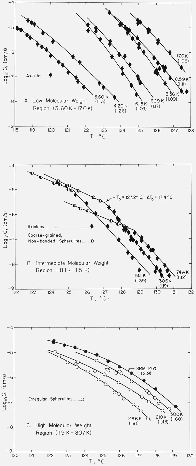
Numbers in parentheses ( ) indicate M_w/M_n for the specimen.

Data are shown for fractions 18.1 to 74.4 K in figure 1B. These specimens are typical of what we term the “intermediate” molecular weight range, which extends from 18.1 to 115 K. It is seen that a definite break occurs in the log₁₀ G versus T data at a temperature that we denote T_b (fig. 1B). Somewhat above T_b, axialites are formed, and somewhat below it only spherulites are seen. (Details of the morphology will be given subsequently.) In the region of intermediate molecular weight, the slopes of the log₁₀ G versus T plots for the axialites are more nearly constant with molecular weight than they were in the low molecular weight range. As in the case of the low molecular weight region, data for a number of other samples were obtained, but are not shown.

In this paper we adhere to the convention of showing axialite data as solid diamonds (♦), coarse-grained non-banded spherulites as half-filled circles (◐), and “irregular” spherulites (see below) as open circles (○).

Before discussing the growth rate data for the “irregular” spherulites that appear in the high molecular weight region, it is advantageous to show that the undercooling at which crystallization is carried out determines whether axialites or spherulites appear in the low and intermediate molecular weight regions.

The variation of T_b with molecular weight as determined from plots of log₁₀ G versus T is shown in figure 2A. It is seen that the break in the growth curves can be clearly detected for samples in the intermediate molecular weight range of M_w= 18,100 to M_w=114,500. This feature is clarified if the under-cooling ΔT_b at which the transition takes place is plotted as a function of molecular weight. The result is that the transition occurs at essentially a fixed undercooling of 17.5 ± 1 °C as is shown in figure 2B. Although the rate transitions at T_b are sharper than the corresponding morphological changes (see below), it is nevertheless found that if the undercooling is about 1 °C or more lower than ΔT_b axialites are formed, and if it is about 1 °C or more greater than this, spherulites are formed. On the basis of this finding, we surmised that spherulites might be found in the specimens witha molecular weight below M_w ≅ 18,000 if crystallization with an undercooling larger than 17.5 °C could be achieved. Runs could not be made on samples lower in molecular weight than 18,000 at ΔT > 17.5 °C because the growth rates became too rapid to measure with any certainty and there is some question as to whether the growth is isothermal under such conditions, but quenching of specimens of such low molecular weight from the melt to room temperature did in fact lead to (nonisothermal) growth of spherulites. The finding that ΔΓ/, = 17.5 °C approximately separates the axialitic and spherulitic growth modes does not applytosamples exceeding about 115 Kin molecular weight. At these high molecular weights, a different type of morphology appears over the entire range where isothermal growth can be effected (“irregular” spherulites), and there is no break in the logjoG versus T curve.

Figure 2. Growth temperature and undercooling; corresponding to break in log G versus T data.

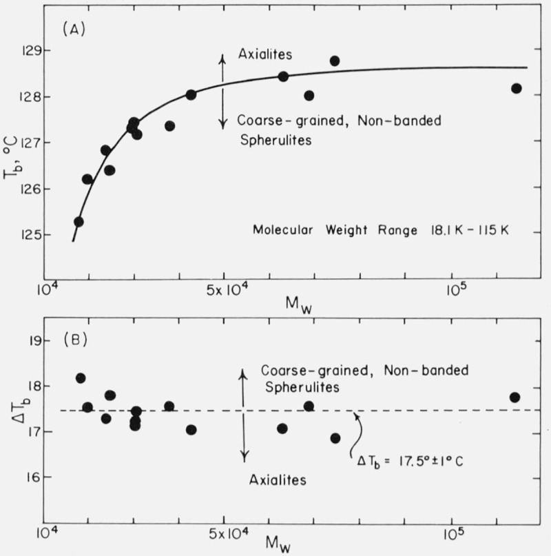
T_b and ΔT_b correspond within about 1 °C to the temperatures and undercoolings that separate the axialitic and spherulitic growth modes.

The values of T°_m as a function of molecular weight used to estimate ¿>_b for the various specimens shown in figure 2B can be obtained from a modified Broadhurst [12] or Flory-Vrij [13] equation (discussed later).

The growth rate of the axialites and coarse-grained non-banded spherulites studied in the low and intermediate range of molecular weight was in every case lineal, i.e., dx|dt at a given temperature is a constant regardless of the size of the spherulite or axialite up to the point of impingement. (The measurements leading to values of G were generally confined to values of x far short of actual impingement.) There was no significant induction period — the x, t data passed through the origin on an x versus t plot within acceptable statistical limits.

Typical growth rate data for the “irregular” spherulites that appear in the high molecular weight region (119 to 807 K) are shown in figure 1C.

A notable feature of the irregular spherulites is that no break is found in the log₁₀G versus T data near ΔT_b=17.5 °C. Instead, each log₁₀G versus T plot exhibits considerable curvature and has an average slope that is between that for the axialities and the coarse-grained nonbanded spherulites (compare figs. 1B and 1C).

It is possible that the absence of a relatively sharp break in the log₁₀G versus T data for the specimens of high molecular weight exhibiting “irregular” spherulites may be associated in part with a broad distribution of molecular weights. This can be seen from a comparison of the data in figure 1 and table 1. Most of the specimens in the “intermediate” range in table 1 possess an M_w/M_n ratio of ~ 1.1 to ~ 1.4 and virtually all exhibit a clear-cut break in the log₁₀G versus T data of the type shown in the examples depicted in figure 1B. On the contrary, most of the specimens in the high molecular weight range where irregular spherulites appear have an M_w/M_n ratio of ~ 1.4 to ~ 1.8, and specimens of this class show an overall large curvature rather than a distinct break in a plot of log₁₀G versus T. One possible implication is that a broad distribution of molecular weights may cause the break at T_b to become quite diffuse in the high molecular weight specimens. Note in figure 1C that the SRM from which the fractions were made, for which M_w ≅ 53,000 and M_w/M_n ≅ 2.90, exhibits a distinct curvature rather than a break. It may be recalled that a narrow molecular weight fraction with M_w=53,000 would be expected to have a distinct break in the log₁₀G versus T curve (fig. 1B). However, it must be pointed out that specimen 119 K, which has a moderately narrow distribution (M_w/M_n = 1.26), shows no break in log₁₀G versus T, while specimen 115 K with a broad distribution of molecular weight (Mw/Mn= 1.61) exhibits the break. This suggests as an alternative that the onset of the appearance of irregular spherulites and the absence of a rather sharp break in the log₁₀G versus T data may be an inevitable result of increasing molecular weight rather than mainly a function of the distribution. The question concerning how high in molecular weight the sharp break at T_b actually occurs and where irregular spherulites appear will probably only be answered when fractions with M_w/M_n ~ 1.1 to 1.2 are available in the high molecular weight range, and measurements made over a considerable temperature range.

The overall radial growth of the irregular spherulites is lineal with time, but possesses an apparent small scale (circa 10 μm) sporadic character in that small sectors at the outer boundary of the irregular spherulite appear to grow for a time, stop, and then begin again. This is possibly a result of the details of the extinction pattern that accompany the outward growth of the lamellae rather than an actual starting and stopping of the growth process.

3.2. Morphology

We first examine the question of morphology for samples in the low and intermediate ranges of molecular weight. Figure 3 shows representative axialites in specimens 7.84, 18.1, 30.6, and 42.6 K.⁶ Note that in each case the undercooling is less than 17.5 °C. Although differences are detectable, it is clear that these structures are rather similar. Figure 4A, 4B, and 4C depicts typical coarse-grained non-banded spherulites in specimens 18.1, 30.6, and 62.8 K. Observe that the undercooling exceeds 17.5 °C in each case. The “maltese cross” effect is present in the extinction pattern, but the spherulites exhibit a coarse texture and are either non-banded or alternatively, have a few very coarse bands. Typical banded spherulites with many concentric rings can be formed by strong quenching from the melt of the samples in the intermediate molecular weight range. An example is shown in figure 4D for specimen 30.6 K, which crystallizes by formation of such spherulites when quenched rapidly from T₁ = 155° to 25 °C. The distinctive feature of the present work resides in the fact that both axialites and spherulites were found in different temperature ranges in the same specimen in the intermediate molecular weight range, together with the fact that these objects exhibited significantly different growth rate constants.

Figure 3. Axialites in specimens of low and intermediate molecular weight at ΔT < 17.5 °C (optical micrographs, crossed nicol prisms).

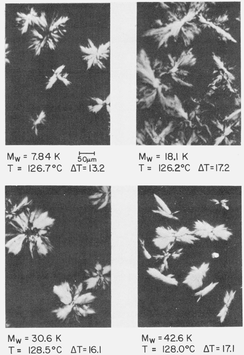
The axialites were grown under isothermal conditions.

Figure 4. Spherulites in specimens of intermediate molecular weight at ΔT > 17.5 °C ,optical micrographs, crossed nicol prisms).

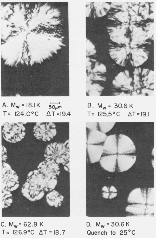
A, B, and C show coarse-grained non-banded spherulites resulting from isothermal growth, ΔT > 17.5 °C. Micrograph D shows typical banded spherulites obtained in specimen 30.6 K by rapid quenching, from T₁= 155 to 25 °C.

From a morphological standpoint, the transitions from axialitic to spherulitic structures observed in the intermediate molecular weight range are not completely abrupt as the undercooling at which the crystallization occurs passes through ΔT_b. However, there are sufficient differences in the appearance of the crystallizing objects 1 °C above and below T_b to warrant classification as a spherulite or axialite. There are smaller variations in the details of structure within each morphology, with the result that the appearance of the spherulites or axialites in an optical microscope can actually be used by an experienced viewer to estimate the crystallization temperature within a degree or so. A set of photomicrographs illustrating the changes of structure with temperatures and degree of undercooling are shown in figure 5 for specimen 30.6 K. The steady change from the coarse-grained non-banded spherulitic morphology at ΔT > 17.5 °C to the axialitic morphology at ΔT < 17.5 °C is clearly apparent. (At the lowest isothermal growth temperature (T= 123.2 °C, ΔT= 21.4 °C) the spherulites show a few coarse bands.) Samples ranging from 18.1 to 74.4 K show rather similar variations of morphology with decreasing undercooling.

Figure 5. Transition from spherulitic to axialitic morphology in specimen 30.6 K with decreasing undercooling (optical micro-graphs, crossed nicol prisms).

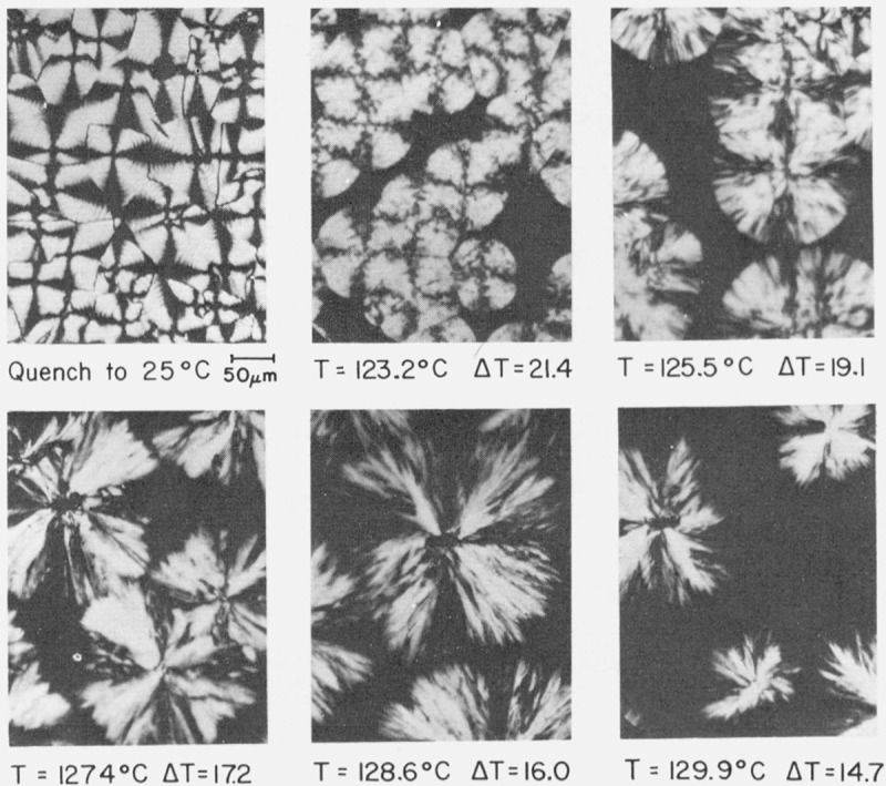
Normal banded spherulites are formed at the large undercoolings effected by quenching. In the ΔT=21.4 °C run there is some evidence of coarse bands. Typical coarse-grained non-banded spheruüties are formed at ΔT= 19.1 °C. The object formed at ΔT=17.2 °C is close to the transition at T_b(see fig. 1B). Axialites are formed at ΔT=l6.0 °C.and ΔT= 14.7°C. Isothermal growth applies in all cases except that denoted quench.

It is worth noting the somewhat unusual structures and phenomena that occur in the specimens in the “high” molecular weight range, i.e., those from 119,000 to near 807,000 in molecular weight. Figure 6 shows the crystalline objects that appear in specimens 119, 210, 323, and 807 K. The clear-cut axialitic morphology characteristic of somewhat lower molecular weights does not appear at undercoolings less than 17.5 °C, and the type of coarse-grained non-banded spherulite seen at intermediate molecular weights at undercoolings greater than 17.5 °C is also absent. Instead, somewhat irregular objects with either a weak or nonexistent “maltese cross” extinction effect appear that in many respects resembles a cauliflower (fig. 6). Some of them show evidence of being banded. We refer to these objects as “irregular” spherulites. The unusual spherulites found for specimen 119 K seem to be a transitional type; the optical micrographs seen in figure 6 for specimens 210, 323, and 807 K are more typical of the “high” molecular weigh, range.

Figure 6. Irregular spherulites in specimens of high molecular weight (optical micrographs, crossed nicol prisms).

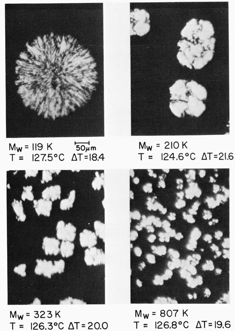
The spherulite in 119 K appears to represent a transition between the intermediate and high molecular weight types. The irregular spherulites in 210 and 323, and 807 K are typical of those found in the high molecular weight region. Growth is under isothermal conditions in all cases.

Some very high molecular weight specimens where M_w > 10⁶ were prepared and examined (not listed). No objects clearly identifiable in an optical microscope with crossed nicol prisms appeared at all despite the fact that differential thermal analysis (DTA) measurements clearly showed that significant crystallization had taken place. Heating of such specimens even for long periods of time to T₁ = 155 °C or even T₁ = 190 °C failed to remove the birefringence so that any crystalline object that appeared on subsequent cooling was impossible to observe properly with an optical microscope. The highest available molecular weight specimen showing any object whose growth rate could be measured was 807 K.

3.3. Birefringence and X-Ray Studies

Birefringence measurements were made on specimens 11.67 K (axialites), 30.6 K (both axialitic and spherulitic regions), and 500 K (irregular spherulites). In each case the sign of the birefringence showed that the polymer chain axes were approximately perpendicular to the direction of growth. This result has been adduced previously for spherulites in polyethylene.

An investigation of sample 30.6 K was made in both the axialitic and spherulitic regions using wide-angle x-ray (WAXR) techniques. The WAXR studies of specimen 30.6 K showed that both the axialitic and spherulitic forms consisted principally of crystals with the usual orthorhombic subcell. The WAXR lines of the axialitic and spherulitic specimens were almost indistinguishable even when examined in detail. The transition from axiahtic to spherulitic growth centering around T_b therefore does not involve crystaUization into different unit subcells above and below T_b

Each specimen showed weak extra WAXR lines that have been assigned to either the monoclinic or the triclinic subcell by various authors [14–16]. These weak “extra” lines are commonly found in melt-crystallized polyethylene [14–16]. Similar WAXR studies were made on the axialites in a low molecular weight specimen (11.74 K) and on the irregular spherulites in a high molecular weight specimen (500 K) with the finding that the orthorhombic subcell was by a wide margin the predominant one present.

Low-angle x-ray (LAXR) studies were also made on sample 30.6 K crystallized at undercoolings corresponding to the axialitic and spherulitic regions. For LAXR studies on specimens 11.74 K and 500 K, the samples were crystallized in 1 to 1.5 mm capillary tubes at a known temperature to a high degree of crystallinity, cooled to room temperature, and the LAXR lines measured there. In one case (30.6 K) the LAXR lines were also measured in a specially designed and thermostated beryllium cell at the actual temperature of crystallization.

The results of the LAXR studies are shown in table 2. In general, the specimens showed two categories of LAXR spacings. The first and most prominent was L₁ (which was usually circa 400 to 600 Å), and its higher orders. The L₁ line is relatively narrow and intense, and its higher orders, when reported in table 2, are also distinct and easily detected. (We note, however, that the L₁ line for 500 K is considerably broader than that found in the specimens of lower molecular weight.) In sample 30.6 K, crystallized at 128.3 °C and cooled to 30.2 °C, four orders of L₁ could be clearly identified (table 2). The second category was the very broad and rather weak so-called “L₂” line, which does not appear to be a higher order of L₁ [17]. Later we will tentatively identify L₂ with the initial lamellar thickness. Melting point data on the specimens discussed here suggest that lamellar thickening (approximately a doubling and sometimes more) occurs in the fractions during crystallization, so it is not surprising that evidence of two different thickness ranges for the lamellae is found in a given specimen (see L₁ and L₂ values in table 2). (In brief, we postulate that L₁ represents thickened (i.e., aged) stacks of lamellae, while L₂ represents the younger unthickened lamellae characteristic of the initial thickness.) Observe that the values of L₂ are mostly in the range of ~ 180 to ~ 220 Å. We note that this is quite close to the theoretical value of the initial lamellar thickness of l_g* = {2σ_eT°_m/(Δh_f)(ΔT)} + C₂ calculated using the effective value of σ_e obtained from the growth rate data (see later).

Table 2.

Low angle x-ray spacings for selected fractions

Specimen	Crystallization temp. °C	Measurement temp. °C	Morphology	X-ray spacingsa
				L1 (Å)	L2 (Å)b
11.74 K	122.0	30.2	Axialites	c368(1)	186(1)
30.6 K	128.3	128.3	Axialites	670(1)	258(1)
30.6 K	128.3	30.2	Axialites	454(4)	195(1)
30.6 K	124.8	124.8	Coarse-grained nonbanded spherulites	396(2)	199(1)
30.6 K	124.8	30.2	Coarse-grained nonbanded spherulites	367(1)	194(1)
500 K	124.0	30.2	Irregular spherulites	470(1)	210(1)

^aThe numbers in parentheses ( ) indicate the number of orders that were detected.

^bThe error in L₂ is rather large, since the line is broad and its value somewhat sensitive to the method used to subtract out the base line.

^cA weak shoulder at ~ 1200±200 Å was observed for this specimen. This appears to correspond to an extended chain structure, and probably results from thickening.

From the LAXR studies noted in table 2 it is seen that both the axialites and coarse-grained non-banded spherulites in the molecular weight range noted (and probably somewhat outside it) are basically lamellar in character. It is also apparent that the irregular spherulites have a lamellar texture.

It has been demonstrated that the spherulites in rather broad molecular weight distribution samples of melt-crystallized polyethylene possess a birefringence consistent with the chain axes in the crystal being perpendicular to the direction of growth [18]. (This same orientation is shown by microbeam x-ray data [19, 20].) Further, it is known that the spherulites in broad distribution material are basically lamellar in character [21], and the same appears to hold for certain fractions [22]. The axialites and spherulites found in the fractions used in the present study show these same general characteristics, which are thus consistent with lamellar crystallization with chain-folding. In order for the argument for chain-folding to be logically complete, it would be necessary to show that the lamellae in each of the morphological variations were parallel to the direction of growth, or to in some other manner demonstrate that the chain axes in the crystal were perpendicular to the large surfaces of the thin lamellae. This has been shown for spherulitic structures in bulk polyethylene with a rather broad molecular weight distribution [23, 24]. Also, Bank and Krimm indicate that the usual type of spherulites in polyethylene exhibit mostly adjacent reentry type chain folding [25]. (For a full discussion of these topics, see the recent review by Khoury and Passaglia [26].)

Because of the parallelism of the optical behavior and lamellar character of the axialites and spherulites found in the present investigation of fractions with the optical and lamellar nature of spherulites where chain folding has been substantiated for broader distribution material, we proceed with some confidence under the assumption that the fractions exhibit chain-folding with mostly adjacent reentry.

4. Analysis of Data to Obtain K_g and G_o

The kinetic theory of nucleation-controlled polymer crystal growth with chain folds leads to the expression [1–3]

$$G=G_0\text{\hspace{0.17em}exp}\left[-U^{*}/R\left(T-T_{\infty }\right)\right]\text{\hspace{0.17em}exp}\left[-K_g/T(\Delta T)f\right]$$ (1)

for the growth rate G. Here U* is the activation energy for transport of segments to the site of crystallization, R the gas constant, T the crystallization temperature, T_∞ a temperature somewhat below the glass transition temperature T_g, ΔT the undercooling T°m-T, and f factor near unity that accounts for the slight diminution of the heat of fusion Δh_f as the temperature falls below T°_m.⁷ By plotting log₁₀G + U*/2.303R(T-T_∞) against 1/T(ΔT)f, the numerical value of the nucleation constant K_g can be obtained from the slope, and the pre-exponential factor G₀ can be determined from the intercept on the log₁₀G + U*/2.303R(T-T_∞) coordinate.

It has been demonstrated by Suzuki and Kovacs [27] that eq (1) quantitatively fits the growth rate data for isotactic polystyrene for a range of 100 °C. In a recent review [1], this result has been confirmed, and it was shown further that eq (1) can be used to fit data on a number of polymers crystallized from the melt over a wide range of temperature with considerable accuracy, including nylon 6, poly(tetramethyl-p-silphenylene) siloxane (hereafter denoted TMPS) fractions, and poly(chlorotrifluoroethylene), correlation coefficients ranging from 0.985 to 0.999 being found. In the aforementioned review, and in the work of Suzuki and Kovacs, it was found that U^* ≅ 1500 cal/mol and T_∞ ≅ T_g - 30 °C, with one exception, allowed the best fit of the rate of crystallization data at low temperatures. (The values of U^* and T_∞ that describe bulk viscous flow in polymers between T_g and T_g +100 °C are U* ≅ 4100 cal/mol and T_∞ ≅ T_g — 51.6 °C. The fact that U*= 1500 cal and T_∞ ≅ T_g — 30 °C for crystallization has been interpreted in terms of segmental motions in an adsorbed polymer layer on the lateral face of the crystal [1].) In the case of the present analysis to obtain K_g and G₀ for various polyethylene fractions, the crystallization rate is controlled much more strongly by the variation with temperature of the term involving K_g/T(ΔT)f than that involving U*/R(T—T_∞), since the region of observable crystallization rates in polyethylene is near the melting point. The variation of U*/R(T—T_∞) is small and that of K_g/T(ΔT)f quite large in this region. Therefore in the case of polyethylene, little error in K_g results from rather large variations in the assumed value of U* or T_∞, and we proceed on the basis of U* = 1500 cal/mol and T=T_g-30 °C, where T_g = −40 °C = 233.2 K [28]. (The assumption that T_g was —80 °C or 193.2 K would lower K_g for a given set of data by only about 2 percent, and the use of U* = 4120 cal instead of 1500 cal would raise K_g by only 5 percent.) The value of f is approximated [1] by f=2T/(T°_m + T). This correction is also quite small for polyethylene, again because the observable isothermal crystallization occurs so near the melting point.

One important parameter that requires discussion is the equilibrium melting temperature T°_m, which is a function of molecular weight. This must be known with the best possible accuracy, since K_g, through its relationship to the undercooling T°_m—T, is rather sensitively dependent upon it. In figure 7 is shown a plot of T^¤_m against molecular weight M calculated using a modified form of Broadhurst’s equation [12]. The expression used to calculate the curve is

$$T_m^{°}=\frac{T_m^{°}(\infty )(n-0.542)}{n+0.46\left\{7.667+1.987\text{\hspace{0.17em}ln\hspace{0.17em}}n+(5.6/n)-(0.25n-7)\left[1-\left(T_m^{°}/T_m^{°}(\infty )\right)\right]\right\}}$$ (2)

where T^¤_m is in kelvins (K), and n=M/14.026 is the number of carbon atoms in the polymer chain. This equation was derived from Broadhurst’s work by setting T^¤_m at n → ∞ at T^¤_m(∞) = 419.7K = 146.5 °C, and adjusting the constants accordingly. The curve calculated with eq (2) passes through the melting point data for the short chain hydrocarbons in the orthorhombic form with acceptable accuracy. Therefore, if the value of T_m(∞) can be justified within certain limits, considerable confidence can be placed on the interpolated values of interest here. Broadhurst’s equationis based on a treatment due to Flory and Vrij [13], and the two treatments differ only in minor details.

Figure 7. Variation of T°_m with molecular weight according to equation (2).

The experimental justification for selecting T^¤_m(∞) = 146.5 °C is as follows: (1) Huseby and Bair [29] found T^¤_m = 145.8 °C± 1 from a plot of T_m versus 1/l where l is the lamellar thickness for polyethylene single crystals with M_w ~ 20,000 to 100,000, implying a T^¤_m (∞) that is about 0.5 to 1 °C higher, (2) a plot of T_m versus T_x obtained by Weeks [30] for melt crystallized polymer suggests T^¤_m =145.5±1 °C for a specimen of finite molecular weight, again suggesting that T^¤_m(∞) for polyethylene of very high molecular weight is slightly higher, and (3) Rijke and Mandelkern [31] have found a melting point for fibrillar polyethylene of T^¤_m = 146.0 ±0.5 °C. We note also that our suggested value for T°_m(∞) lies within the limits given by Flory and Vrij, who give T°_m(∞)ι=145.5±l °C. In any event, it seems reasonable on the basis of the above to assume that Tm(∞) is within about 1 °C or so of 146.5 °C. No basic conclusion of this paper would be changed if a different value of T°_m(∞) in this range were used or even a value somewhat outside of it. The melting point T°_m for each fraction was estimated using the assumption that the M value implicit in eq (2) corresponds to M_w. Numerical values of T°m calculated using eq (2) are given for each of the fractions in table 1.

Typical plots of log₁₀G+U*/2.303R(T-T_∞) against l/T(ΔT)f constructed from low molecular weight data of the type shown in figure 1A are shown in figure 8A. As noted earlier, only axialites are found in low molecular weight samples in the range of undercooling where isothermal runs can be made. Similar plots for a number of the samples of intermediate molecular weight based on data of the type shown in figure 1B are depicted in figure 8B. Both axialites and coarse-grained non-banded spherulites appear in this molecular weight region at the undercoolings noted. It is clear from the slopes that the axialites and spherulites have different nucleation constants. Finally, a plot is shown for some of the irregular spherulites found at high molecular weight in figure 8C.

Figure 8. Typical plots of log₁₀ G + U*/R(T—T_∞) versus 1/T (ΔT)f in low, intermediate, and high molecular weight regions. Numbers in parentheses () indicate M_w/M_n.

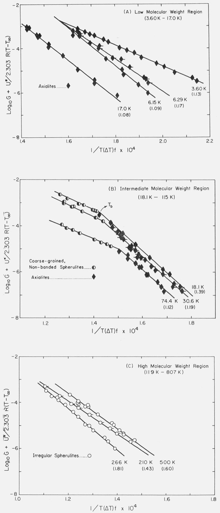
The growth rate G is in units of cm/s.

Values of the nucleation constants K_g obtained from plots such as those shown in figure 8 are shown for all specimens studied in figure 9A. Values of K_g and log₁₀ G₀ are given in table 3. The error in the K_g for a given fraction was generally about 3 to 5 percent (calculated as one standard deviation), depending on the number of points and the temperature range involved. To test the reproducibility of our procedures, a portion of the original supply of sample 30.0 K was rerun, including all filtration, optical sample preparation, and growth rate measurement steps. The K_g for the axialites was within 1.7 percent of the previous run, while that for the coarse-grained non-banded spherulites was within 2.6 percent (table 3). Based on this and other reruns (table 3) it is believed that the K_g values are in general correct to within about 3 to 5 percent. In a few cases the error is larger, and these values of K_g are enclosed in parentheses in table 3.

Figure 9. Experimental values of K_g and log₁₀G₀ as a function of molecular weight. G₀ is in cm/s and K_g is in units of K².

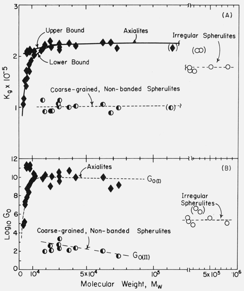
Table 3.

Values of K_g, log₁₀G₀ and σσ_e for various polyethylene fractions

Sample designation	Mw/Mn	Temperature range	Kg × 10−5	Log10 G0	σσe calc. with b=4.15 Å using $\frac{K_{g\left(I\right)}=4b\sigma {\sigma }_e{T}_m^{°}/\Delta h_{f}k}{\begin{array}{l}{\text{erg}}^2/{\text{cm}}^4\hfill \end{array}}$
A. Low molecular weight region (axialites)
		°C	K2	(G0 in cm · s−1)
3.6 K	1.13	117.6–121.9	1.069	4.97	611
4.2 K	1.26	118.7–123.7	1.172	5.14	668
5.10 K	1.10	119.9–124.3	1.516	7.37	861
5.62 K	1.05	119.8–124.7	1.434	7.15	812
6.15 K	1.09	122.1–124.9	2.101	11.28	1188
a6.15K(R)	1.09	122.1–124.9	2.078	11.10	1176
6.29 K	1.17	122.6–125.1	1.725	8.81	976
6.35 K	1.06	120.0–125.2	1.578	7.86	892
7.84 K	1.03	121.7–126.7	1.714	8.41	966
8.06 K	1.12	122.7–126.3	1.830	9.07	1031
8.56 K	1.09	123.4–126.5	2.127	11.23	1197
a8.56 K(R)	1.09	123.4–126.5	2.098	11.01	1181
8.59 K	1.11	124.3–127.8	1.822	9.30	1025
9.70 K	1.06	124.3–127.5	1.935	9.56	1087
11.4 K	1.09	124.2–127.7	2.078	10.39	1166
11.67 K	1.09	125.0–127.6	2.0%	10.01	1175
11.74 K	1.07	125.3–128.5	2.036	10.17	1142
17.0 K	1.08	125.0–128.9	2.098	9.75	1173
B. Intermediate molecular weight region (axialites, ΔT < 17.5 °C)					σσe calc. with b=4.15 Å using $\frac{K_{g\left(I\right)}=4b\sigma {\sigma }_e{T}_m^{°}/\Delta h_{f}k}{\begin{array}{l}{\text{erg}}^2/{\text{cm}}^4\hfill \end{array}}$
18.1 K	1.39	125.2–129.1	2.152	9.88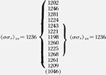
19.8 K	1.07	126.2–129.1	2.231	10.23
23.7 K	1.07	126.8–130.0	2.296	9.04
24.6 K	1.07	126.4–129.6	2.195	10.07
30.0 K	1.12	127.4–128.9	2.230	10.50
a30.0 K(R)	1.12	127.4–129.4	2.192	10.12
30.6 K	1.19	127.2–130.3	2.150	9.60
37.6 K	1.10	127.3–130.0	2.263	10.70
42.6 K	1.22	128.0–129.8	2.202	10.00
62.8 K	1.37	128.4–130.5	2.280	9.98
68.6 K	1.17	128.0–129.7	2.268	8.77
74.4 K	1.12	128.8–130.8	2.175	9.21
115 K	1.16	128.1–130.7	(1.883)	(6.76)
C. Intermediate molecular weight region (coarse-grained non-banded spherulites, ΔT < 17.5 °C					σσe calc. with b=4.15 Å using $\frac{K_{g\left(II\right)}=2b\sigma {\sigma }_e{T}_m^{°}/\Delta h_{f}k}{\begin{array}{l}{\text{erg}}^2/{\text{cm}}^4\hfill \end{array}}$
18.1 K	1.39	122.9–125.2	1.142	3.63
19.8 K	1.07	125.8–126.2	0.932	2.00
23.7 K	1.07	124.6–126.8	.942	2.60
24.6 K	1.07	124.8–126.4	.925	2.12
30.0 K	1.12	124.8–127.4	1.065	2.71
a30.0 K (R)	1.12	125.0–127.4	1.038	2.34
30.6 K	1.19	124.4–127.2	1.141	3.33
37.6 K	1.10	124.6–127.3	1.008	2.13
42.6 K	1.22	124.8–128.0	1.028	2.36
62.8 K	1.37	125.9–128.4	1.061	2.06
68.6 K	1.17	125.6–128.0	(0.896)	(0.51)
74.4 K	1.12	125.4–128.8	0.998	1.49
115 K	1.61	125.6–128.1	1.042	1.66
D. High molecular weight region (irregular spherulites)					σσe calc. with b=4.15 Å using $\frac{K_{g\left(\text{I,II}\right)}=3b\sigma {\sigma }_e{T}_m^{°}/\Delta h_{f}k}{\begin{array}{l}{\text{erg}}^2/{\text{cm}}^4\hfill \end{array}}$
119 K	1.26	125.3–129.4	1.777	5.64
134 K	1.70	123.1–128.5	1.725	5.21
210 K	1.43	122.4–128.4	1.710	4.86
266 K	1.81	122.6–127.6	2.113	(6.63)
323 K	1.61	120.3–126.3	2.113	(6.31)
500 K	1.60	125.0–129.1	1.795	5.61
807 K	1.59	124.5–129.3	1.800	5.08

^a(R) denotes complete rerun.

^bCalculated with regime I kinetics. (See text.)

Attention is specifically drawn to the apparent scatter of the K_g data in figure 9A and table 3 at closely spaced molecular weight values at low molecular weights, especially near M_w= 6200 and M_w = 8600. Note particularly specimen pairs (6.15, 6.29 K) and (8.56, 8.59 K), together with the confirmatory reruns of the high points, 6.15(R) and 8.56(R). This “scatter” is definitely outside the estimated experimental error of the K_g data. The large variation in K_g at these low molecular weights is believed to be associated with cilium length effects, and will be discussed in section 6.

For the axialites, the value of K_g generally rises at first and then tends toward a limiting value at about M_w = 20,000, and remains approximately constant within experimental error up to the highest molecular weight where an accurate axialite run can be made (M_w ~ 72,400). In the case of the coarse-grained non-banded spherulites, the K_g values are approximately constant in the molecular weight range where their growth can be observed (M_w ≅ 18,000 to M_w ≅ 115,000). From an experimental standpoint, the most accurate values of K_g for the coarse-grained non-banded spherulites lie between M_w =30,000 and M_w=62,800. The K_g value for the axialites in sample 115 K shows some evidence of being affected by the transition to high molecular weight behavior; sample 119 K exhibits no axialites and has no T_b at all.

The values of log₁₀G₀ obtained from the intercepts on the ordinate of plots of the type shown in figure 8C are shown in figure 9B. Because of the long extrapolation, the scatter in the log₁₀G₀ data is rather large. It is estimated that each G₀ value is correct to within about one order of magnitude. However, there are differences between the results for axialites, non-banded spherulites, and irregular spherulites that are far outside this error limit, and which are amenable to theoretical interpretation (see sec. 6).

5. Regime I and Regime II Growth: Calculation of σσ_e from K_g

5.1. Relationship Between Surface Nucleation Rate i and Regime I and Regime II Crystal Growth Rate Laws

The rate of deposition i of chain-folded nuclei on a unit length of a substrate is given by nucleation theory as [1, 2]

$$i(\text{surface nuclei\hspace{0.17em}}\cdot {\text{sec}}^{-1}\cdot {\text{cm}}^{-1})=C\beta \text{\hspace{0.17em}exp}\left[-4b\sigma {\sigma }_e/(\Delta f)kT\right]$$ (3)

where β is a retardation factor measured in units of “events” or “nuclei” per second that has a temperature dependence of the form exp [-U*/R(T-T_∞)], C is a constant, in units of cm⁻¹, that is essentially independent of temperature, and (Δf) the free energy difference between the subcooled liquid and the crystal. In general, (Δf) is given by (Δh_f)(ΔT)f/T°_m, where for a number of polymers including polyethylene, f ≅ 2T/(T°m + T). (In the case of crystallization of polyethylene from the melt, the factor f never differs more than 3 percent from unity. However, in the case of homogeneous nucleation, where ΔT is typically 60 °C, this factor is of considerable importance in obtaining correct estimates of σ²σ_e.) Thus the surface nucleation rate may be written [1, 2]⁸.

$$i=\beta (z/a)\text{\hspace{0.17em}exp}\left[-4b\sigma {\sigma }_e{T}_m^{°}/\left(\Delta h_f\right)(\Delta T)kTf\right].$$ (4)

where for polyethylene z is the number of —CH₂ — units corresponding to the initial lamellar thickness l*_g. In rough calculations we may take l*_g as 200 Å, giving z ~ 158; the quantity a is the molecular width, which is 4.55 Å for polyethylene for growth where folds form along the (110) planes (i.e., the long diagonal) of the unit cell. This corresponds to a layer thickness b of 4.15 Å.⁹

With such a surface nucleation rate, one can imagine two limiting cases for the rate of growth normal to the substrate which depend on the nucleation rate itself and the rate g that the folded nucleus spreads on the substrate. It is important to examine these possibilities, since it will be found that both occur in polyethylene.

5.2. Regime I (Single Surface Nucleus Causes Completion of Substrate)

The customary assumption is that each nucleation act causes the substrate or “persistence” length L to be completed before a new surface nucleus appears, leading to the accession of a new layer of thickness b (fig. 10). The growth rate G normal to the substrate is in this case given by G=biL. The quantity L is given by n_sa, where n_s is the number of available stems where crystallization may begin on the substrate (fig. 10).¹⁰ In any event, one readily finds in cases where G ∝ i that [1, 2]

$$G_{\text{I}}=G_{0\left(\text{I}\right)}\text{\hspace{0.17em}exp}[-U^{*}/R\left(T-T_{\infty }\right)]\text{\hspace{0.17em}exp}\left[-4b\sigma {\sigma }_e{T}_m^{°}/\left(\Delta h_f\right)(\Delta T)kTf\right].$$ (5)

Figure 10. Regime I and regime II growth (schematic).

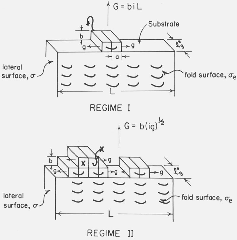
The quantity L is equal to n_sa, where n_s is the number of stems of length l*_g comprising the substrate, and a the width of each molecule.

To a sufficient approximation the pre-exponential factor is given by

$$G_{0(\text{I})}\cong b(kT/h)n_{s}z{J}_1=b(kT/h)(L/a)z{J}_1,$$ (6)

where J₁ is a factor that was anticipated in previous work [l, 2] to be within perhaps two orders of magnitude of 10⁻³. Observe that G_0(I) contains the factor n_s which depends on the mean substrate or “persistence” length L. In previous work n_s was estimated to be 10³ to 10⁶ [2]. Note that n_sz is the number of —CH₂ — units on the substrate, i.e., the number of “sites” where crystallization of a new layer can be initiated.

By comparison with eq (1) and eq (5), it is seen that

$$K_{g(\text{I})}=4b\sigma {\sigma }_e{T}_m^{°}/\left(\Delta h_f\right)k.$$ (7)

5.3. Regime II (Numerous Surface Nuclei Involved in Formation of Substrate)

Under certain circumstances to be discussed shortly, it is not reasonable to suppose that the substrate will be completed before many other nuclei impinge on it (fig. 10). Thus we consider the other limit where the surface nucleation rate i is very large compared to the spreading rate g for a specified L. Sanchez and DiMarzio [7] and more recently Lauritzen [8] have shown that the growth rate normal to the substrate in this case is (omitting a numerical factor of the order of unity) given by G=b(ig) ^1/2. Noting that the spreading rate is to a sufficient approximation given by [2]

$$g=a\beta \text{\hspace{0.17em}exp}\left[-2ab{\sigma }_e/kT\right]$$ (8)

it can be shown that

$$G_{\text{II}}=G_{0\left(\text{II}\right)}\text{\hspace{0.17em}exp}\left[-U^{*}/R\left(T-T_{\infty }\right)\right]\text{\hspace{0.17em}exp}\left[-2b\sigma {\sigma }_e{T}_m^{°}/\left(\Delta h_f\right)(\Delta T)kTf\right]$$ (9)

where to the same approximation that was used for G_0(i),

$$G_{0(\text{II})}=b(kT/h)z^{1/2}{J}_1\text{\hspace{0.17em}exp}\left[-ab{\sigma }_e/kT\right].$$ (10)

Note that G_0(II) does not contain the factor L or n_s. The ratio

$$\frac{G_{0\left(\text{I}\right)}}{G_{0(\text{II})}}=n_s{z}^{1/2}\text{\hspace{0.17em}exp}\left(ab{\sigma }_e/kT\right)$$ (11)

shows that G_0(I) must under comparable conditions always be larger than G_0(II).

The value of K_g for regime II has the value

$$K_{g(\text{II})}=2b\sigma {\sigma }_e{T}_m^{°}/\left(\Delta h_f\right)k$$ (12)

which differs from that for regime I by a factor of two. This arises fundamentally from the fact that G_I∝ i, while G_II∝i^1/2.

We turn now to the question of which formula, eq (7) or eq (12), should be used to estimate σσ_e from an experimentally known value of K_g.

5.4. Criteria for Regimes I and II

Lauritzen [8] has shown that when the dimensionless quantity

$$Z=i{L}^2/4g$$ (13)

is 0.01 or less that regime I holds with high precision, in which case eqs (5–7) apply. If Z = 0.1, the K_g for regime I is correct to within about 10 percent. Conversely, we estimate that when Z ≥ 1 that regime II is entered, and is closely followed when Z >> 1. Thus for a given substrate length L, the ratio i/g determines which regime of crystallization is applicable. When i/g is large, regime II kinetics hold, and when i/g is small, regime I kinetics obtain. The principal variation of Z with temperature is a result of the large variation of i with undercooling.

The test for regime I and regime II behavior is as follows. We consider the experimental value of K_g, as obtained by analysis of data with eq (1) to be known. We may now write [1, 2]

$$Z=i{L}^2/4g\approx zW{(L/2a)}^2\text{\hspace{0.17em}exp}[-X/T(\Delta T)]$$ (14a)

where

$$X=K_g\text{ (experimental)\hspace{0.17em}for test of regime I with }Z⩽0.1$$ (14b)

and

$$X=2K_g\left(\text{experimental}\right)\text{\hspace{0.17em} for\hspace{0.17em}test of regime II with\hspace{0.17em}}Z\ge 1.$$ (14c)

In the above expression for Z, it is found in one approximation that [1, 2]

$$W=\text{\hspace{0.17em}exp}\left(2ab{\sigma }_e/kT\right).$$ (14d)

With these expressions, it is possible to estimate the range of L values that are consistent with regimeI or regime II behavior. What frequently happens is that such a procedure suggests a reasonable value of L for one regime, and an impossible one for the other, allowing the correct choice of regime to be made by reductio ad absurdum. Examples that illustrate this are cited below. The value of L cannot exceed the dimensions of a small spherulite, which places an upper limit of perhaps 25 to 50 μm on this quantity. The lower limit is at present a matter of speculation, but values of L below about 0.1 μm or 1000 Å are suspect: a predicted value of L that is on the order of the molecular width a is clearly inadmissable.

5.5. Application of Regime Test to Spherulites and Axialites in Polyethylene

We select K_g values for the test that correspond to the molecular weight in the intermediate range of ~ 30,000 to ~ 70,000 where K_g is reasonably near its limiting value (fig. 9 and table 3). Values of the parameters useful in the calculations to follow have been collected in table 4 in the appropriate units.¹¹

Table 4.

Input data for calculations on polyethylene

Quantity	Value	Remarks
Heat of fusion, Δhf	2.80 × 109 erg/cm3	See [1] for original reference
Molecular width, a Layer thickness, b	4.55 × 10−8 cm 4.15 × 10−8 cm	Valid at 125 °C for (110) type growth facea
Cross-sectional area of chain. ab = A0	18.9 × 10−16 cm2	Valid at 125 °C
Fold surface free energy. σe(eq) from Tm vs 1/l plot	93 erg/cm2	Ref. [29]
Number of —CH2— units in stem. z
(calc. for l = 200 Å)	158
(calc. for l=190 Å)	150
Product z exp(2abσe/kT)=zW in eq (14a)	8.96 × 104

^aIf the growth corresponds to (200) type layers, b = 3.82×10⁻⁸ cm and a = 4.95×10⁻⁸ cm at 125 °C.

For the coarse-grained non-banded spherulites in the range 30,000 to 70,000 we use ΔT=20 °C, T=400 K, and X= K_g = 1.05 × 10⁵ K². Then for these objects to obey regime I, it is found with eqs (14a) and (14b) that L≤2Å, which must be regarded as completely unrealistic — no growth could occur on such a substrate. The test for regime II using eqs (14a) and (14c) for these spherulites indicates with X = 2K_g = 2.1 × 10⁵ K² that regime II applies when L ≥ 1.4 μm, which is an entirely reasonable substrate length. It is therefore possible to draw the definite conclusion that the coarse-grained non-banded spherulites in the molecular weight region mentioned grow according to regime II kinetics, in which case K_g is given by 2bσσ_eT^¤_m/(Δh_f)k.

Consider now the corresponding calculations for the axialites in the intermediate molecular weight range, where we may use K_g= 2.2 × 10⁵ K², ΔT= 16 °C and T=400 K to make estimates. It is found that for these objects to obey regime I kinetics (Z≤0.01) then L≤~ 8.1 μm. If the condition Z = 0.1 is used then L≤~ 26 μm. Either way, these are reasonable substrate lengths. A test for regime II behavior with X = 2K_g=4.4 × 10⁵ and Z ≥ 1 gives L≥~ 10⁵ cm, which is absurd. We conclude that the axialites grow according to regime I kinetics, so that K_g=4bσσ_eT°_m/(Δh_f)k must apply.

It is of special interest to comment on the regime that applies to the axialites in the low molecular weight range where K_g falls significantly below the value ~2.2×10⁵ K² typical of the intermediate molecular weight range. Recall that in the intermediate range that the axialites follow regime I kinetics. Theoretically, the low K_g at low molecular weights could be a result of two quite different causes. The first hypothesis is that regime I applies as it does at higher molecular weights and that it is σ_e (viewed as the average surface free energy of cilia and folds) that actually falls, leading to the low K_g value. The second hypothesis is that K_g falls at low molecular weight because regime II is entered, this process taking place in such a way that σ_e is approximately constant. These hypotheses are easily checked using the most extreme axialite case, sample 3.6 K, for which K_g= 1.069 × 10⁵ K². A simple calculation using Z ≥ 1 shows that L would have to be larger than 0.14 cm for regime II kinetics to apply. This is clearly impossible, so pure regime II behavior can be discounted. A test for regime I kinetics using Z ≤ 0.1 indicates that regime I is applicable if L is 1250 Å or less. (In making this estimate, it was assumed in calculating W in eq (14d) that σ_e had fallen to a value of 45 erg/cm².) This may be regarded as perhaps a borderline case of regime I behavior, but specimens of somewhat higher molecular weight give results that clearly imply the applicability of regime I kinetics for the axialites. In all these instances, the occurrence of regime I can be traced to the low undercooling at which axialites grow in specimens of low molecular weight. The average undercooling $\overline{\Delta T}$ for specimen 3.6 K is only 13.6 °C. Thus, in the expression for Z, a low K_g is compensated for by a low value of $\overline{\Delta T}$. It is our conclusion that the falling off of the value of K_g for the axialites in the low molecular weight region is not a result of any serious variation of regime with molecular weight, but is instead caused mostly by a genuine lowering of σ_e as the molecular weight falls. The subject of the variation of σ_e with molecular weight will be dealt with in more detail in subsequent sections.

The case of the “irregular” spherulites that appear from 119 to 807 K is of interest. Using the test value K_g≅ 1.75 × 10⁵ K² from table 3 as X in eqs (14), it is found that the substrate length L is such as to suggest that the samples are crystallizing between regimes I and II. At ΔT = 20, for regime I to apply exactJy (Z ≤ 0.01), then L would have to be less than 150 Å. This is too small a substrate to be fully credible. Under the same conditions of undercooling, L would have to be 0.83 cm or larger to have regime II kinetics. This is much too large to be acceptable. The true value of L almost certainly lies between these extremes, and the samples therefore behave in a manner intermediate between regimes I and II. In this situation we apply the approximate formula

$$K_{g(\text{I,II})}\cong 3b\sigma {\sigma }_e{T}_m^{°}/\left(\Delta h_f\right)k$$ (15)

where the subscript (I, II) means mixed regime I and II behavior, and where it is understood that the factor of 3 contains an inherent uncertainty of perhaps ±1/2.

Two of the irregular spherulite specimens (266 and 323 K) are close to regime I. The rest all fall between regimes I and II as noted above.

5.6. Sharpness of the Regime l → Regime II Transition: An Estimate of L

The relative sharpness of the transition between regimes I and II is evident in figures 1B and 8B, and requires comment. This effect can be understood by plotting Z versus ΔT using

$$Z=i{L}^2/4g\cong zW{(L/2a)}^2\text{\hspace{0.17em}exp}\left[-4b\sigma {\sigma }_e/\left(\Delta h_f\right)(\Delta T)kT\right]$$ (16)

with the constants appropriate to polyethylene given in table 4. As noted earlier, the temperature dependence of Z is controlled principally by the nucleation rate i, which according to eqs (3), (4) and (16) depends on σσ_e. Taking σσ_e to have the nominal value of 1250 erg²/cm⁴, which corresponds to K_g(I)≅2.2×10⁵K², it is easy to calculate Z versus ΔT for various assumed values of L. The results are shown in figure 11 for L values between 1 and 30 μm.

Figure 11. Plot of Z versus ΔT for polyethylene for various substrate or persistence lengths L (theoretical).

Calculated with σσ_e = 1250 erg²/cm⁴, z=158 and other data from table 4 using eq (16). Regime I kinetics are substantially in effect for Z ≤ 0.l; and regime II kinetics are approximately obeyed for Z = 1 and are fully in effect for Z ≥ 10. The shaded area shows region of Z and ΔT where the bulk of regime I → regime II transition takes place.

Consider the curve for L = 5μm. It crosses the line Z = 0.1 at ΔT=17.6 °C, and intersects Z=1 at ΔT=19.2 °C. Regime I is valid within 10 percent for Z=0.1, and regime II is substantially obeyed for Z=1, and obeyed with considerable precision for Z ≥ 10. Thus, we estimate that the bulk of the transition takes place in a temperature range no larger than ~ 1.6 °C. It is also interesting to note that the treatment outlined above suggests that for a fixed value of L the transition should take place at a fixed undercooling, which is what is observed for specimens of different molecular weight (ΔT_b=17.5±l °C, fig. 2B). Assuming that ΔT_b corresponds to Z ~ 0.3, it is found that ΔT_b is about 17.5 °C for L= 10 μm, which is in good accord with the experimental value of ΔT_b=17.5±l °C.

It may be surmised from the above that the value of L near the regime I→ regime II transition is within about a factor of about three or so of 5 μm for polyethylene in the intermediate molecular weight range. The width of the fibrils in polyethylene crystallized from the melt has been reported to be of about this magnitude [22, 32].¹² The value of L may be connected with the existence of a fibrillar habit in polyethylene spherulites — in such a case the width of the fibrils might be governed by L interpreted as a persistence length. Possibly this conception deserves further consideration, but we shall not pursue it further here.

5.7. Calculation of σσ_e as a Function of Molecular Weight from the K_g Values for Various Fractions

The K _g data for the axialites in the low and intermediate range have been analyzed using regime I kinetics according to eq (7) to obtain σσ_e, and the results given in table 3 and plotted in figure 12A. For the axialites, the value of b in the expression for K_g(I) was taken to be equal to b₍₁₁₀₎, i.e.,4.15 Å (table 4). (The symbol b₍₁₁₀₎ refers to the thickness of the layer growing along the (110) planes; this is d₍₁₁₀₎ in the customary crystallographic notation.) This tentative assignment is based mostly on the physical appearance of the axialites, inasmuch as they at least superficially resemble aggregates of single crystals of the type grown from solution. By the use of a linear molecular weight scale, figure 12A emphasizes those results that correspond to the molecular weight range 18,100 to 72,400 where K_g and hence σσ_e is nearly constant with molecular weight. Because of the logarithmic molecular weight scale, figure 12B stresses detailed values of σσ_e calculated for the axialites in the region of low molecular weight where K_g increases noticeably with increasing molecular weight, and where a large variation in σσ_e occurs because of the variation in K_g.

Figure 12. σσ_e and σ_e as a function of molecular weight.

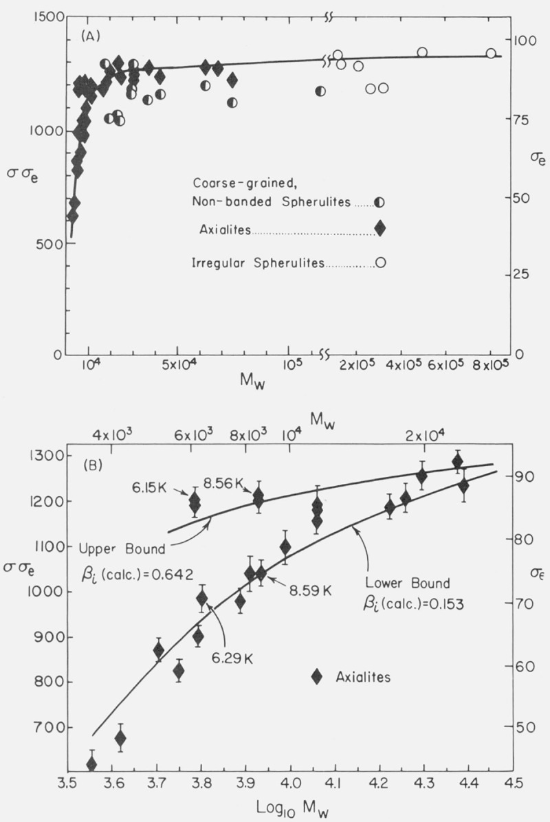
The K_g data for the coarse-grained non-banded spherulites in the region M_w=18,100 to 115,000 were analyzed to obtain σσ_e using regime II kinetics with eq (12). These results are shown in table 3 and in figure 12A. For these spherulites, the value of b in the expression for K_g(II) was taken to be equal to b₍₁₁₀₎, i.e., 4.15 Å (table 4). This assignment of b might seem to contradict the work of Bank and Krimm [25] who found predominantly (200) type folds for spherulites grown at ΔT> 17.5 °C in polyethylene with a broad molecular weight distribution. Actually these folds are parallel to the direction of overall growth, the latter being colinear with the b axis of the unit cell. This leaves open the definite possibility that the leading growth front is really of the (110) type. The work of Bank and Krimm does not preclude the existence of a certain fraction of (110) type folds.¹³

It is evident from figure 12A and table 3 that the σσ_e values for the axialites and coarse-grained non-banded spherulites that occur in the same specimens between 18.1 and 72.4 K are approximately the same despite the fact that the experimental K_g values from which these results were calculated differ by a factor of about two. This is mostly a result of correctly identifying the regime of crystallization in the two cases. In addition, it is clear from figure 9 and table 3 that, in qualitative accord with expectation, the G₀ values for the axialites (regime I) are very much larger than those for the spherulites (regime II) in the same specimens.

With the two exceptions, the K_g, data for the irregular spherulites found between 119 and 807 K were analyzed for the approximate value of σσ_e using eq (15) with b = 4.15 Å and the results given in table 3 and plotted in figure 12A. The exceptions to the use of “mixed” regime kinetics are samples 266 and 323 K, which approximate regime I. Note that the σσ_e values for all these specimens are quite close to what was found for the axialites above M_w ≅ 20,000. The G₀ values for the irregular spherulites are in all cases between those of the axialites and the coarse-grained non-banded spherulites, again suggesting a mixed regime I and II growth mode.

It should be recalled that the numerical value 3 in eq (15) possesses an inherent uncertainty of up to 15 to 20 percent, so the σσ_e values for the “mixed” regime irregular spherulites are not as accurate as they are for the axialites and non-banded spherulites. Nevertheless, it is perhaps somewhat surprising that the advent of interlamellar links on a fairly large scale, which is thought to occur between M_w= 10⁵ and 10⁶, does not affect σσ_e and the corresponding average value of σ_e in a more obvious manner. (An interlamellar link of substantial length must be expected to exhibit a high local surface free energy.) Polyethylene exhibits a marked reduction in degree of crystallinity in this range [33, 34] which has been interpreted partly in terms of the occurrence of a considerable amount of “amorphous” material consisting at least partly of interlamellar links [1]. One possible implication of the above is that the number of such links is small and the amount of material in each one rather large at high molecular weights.

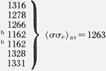
To a fair approximation, the various ranges of K_g values shown in figure 9 for the different morphologies lead to a single master curve for σσ_e for M_w ≥ ~ 20,000 when K_g, is analyzed by taking proper account of the regime of crystallization (fig. 12A). This is especially true of the data for the axialites and the irregular spherulites. The results for the coarse-grained non-banded spherulites appear to be slightly lower than those for the axialites. However, it may be noted that a statistical analysis of the “best” data, which lie between 30.0 and 62.8 K, shows that the coarse-grained spherulites and axialites have slightly overlapping values calculated as one standard deviation: coarse-grained non-banded spherulites, <σσ_e>_av=1177±53 erg²/cm⁴; axialites in the same range, <σσ_e>_av= 1236±26 erg²/cm⁴. The value of <σσ_e>_av for the irregular spherulites is 1263± 58 erg²/cm⁴.

5.8. The Pre-exponenti al Factors for Regimes I and II

Before proceeding to analyze σσ_e to get the molecular weight dependence of σ_e, it is worthwhile to briefly examine the pre-exponential factors for regime I and II. The ratio G_0(I)/G_0(II) as given by eq (11) is independent of J₁, and will be dealt with first. The best data on this ratio encompasses specimens 30.0 to 62.8 K. Here regime I and regime II crystallization occur in the same specimen over a reasonable temperature range for each regime, and the data exhibit good internal consistency within each regime. The ratio log₁₀[G_0(I)/G_0(II)] obtained from the data in table 3 is shown in table 5A, together with the theoretical value calculated using eq (11) for the case L = 10⁻³ cm (10 μm). The result may be regarded as satisfactory in view of the fact that the value of the ratio G_0(I)/G_0(II) is from an experimental standpoint probably not reliable to better than an order of magnitude. In any event, the theory certainly predicts the bulk of the difference in the pre-exponential factors in regimes 1 and II. Most of this difference is a result of the factor n_s, which occurs only in the expression for G_0(I).

Table 5.

Estimates of pre-exponential factors

A. The ratio G0(I)/G0(II)	Log [G0(I)/G1(II)]
Experimental value (30.0 to 62.8 K)	7.66 ± 1.0
Theoretical value for L = 10 μm (eq 11)	6.86
B. Absolute valuesa of G0(I) and G0(II)	G0(I), cm/s	G0(II), cm/s
Theoretical value (with ΔF† = 4.5 kcal/mol;.J1 = 3.6 × 10−3)	0.52 × 1010	0.72 × 103
Experimental value (30.0 to 62.8 K)	1.4 × 1010	0.3 × 103

^aG_0(I) calculated with L = 10 μm.

The absolute values of G_0(I) and G_0(II) depend on J₁ = exp(−ΔF^✝/RT) (see eqs (6) and (10)). For the choice L ≅ 10 μm, which is within the range estimated previously, the most consistent results are obtained when J₁ is set equal to 3.6 × 10⁻³, which corresponds to ΔF^✝ = 4500 cal/mol. Then the absolute values of G_0(I) and G_0(II) are predicted within a factor of no worse than three (table 5B). The factor J₁ was inserted in β = (kT/h) J₁ exp[- U*/R (T- T_∞)] - from which position it enters the absolute growth rate - to account for any orientational or “parking” problem effects that might occur as polymer segments migrate across the substrate to the site of crystallization [1, 2]. The value of ΔF^✝~ 4500 cal/mol is undoubtedly subject to considerable uncertainty. From a theoretical standpoint little can be said of J₁ without a much more detailed model of the surface segmental motions involved in crystallization except to note that it should be substantially less than unity. In the case of the crystallization of copolymers or partially atactic polymers, a “parking” problem arises which should cause J₁ to become considerably smaller than was estimated for polyethylene.

Finally, we comment on the dependence of G₀ on molecular weight. If the absolute growth rate depended on the melt viscosity, one would expect G₀ to vary as M^−3.4. Between Mw ≅ 8500 and Mw= 74,400, the value of G_0(I) for the axialites shows some scatter, but no persistent trend with molecular weight (see fig. 9B and table 3). In this region the melt viscosity increases as M^3.4, i.e., it rises by a factor of (74,400/8500)^3.4 or about 1600 times. It is therefore possible to state with considerable certainty that the absolute growth rate of the axialites, as reflected in the value of G_0(I), is not markedly affected by changes in the macroscopic viscosity. (Recall also that K_g and σσ_e are approximately constant over much of this range.) The theory for β was constructed in such a way as to refer to the “segmental” or “local jump” rate, which depends but little on molecular weight, and this accounts for the fact that G₀ is not predicted to vary strongly with molecular weight [1, 2]. Evidently this assumption was a good one for axialites in the molecular weight range cited. Specimen 115 K shows a low value of log₁₀G₀ in the axialitic region (see table 3), but this sample is very close to the transition region where irregular spherulites appear, and has rather broad distribution.

The situation with the molecular weight dependence of G₀ for the coarse-grained non-banded spherulites that occur between 18.1 and 115 K is not so clear-cut because of the large scatter (fig. 9B). On examination of the data, one nevertheless gains the impression that G₀ for these structures falls as the molecular weight increases. A statistical analysis of all the points suggests that G₀ ∝ M_w^−1.5±0.5. It is extremely unlikely that the variation can be as large as M_w^−3.4, which again means that the melt viscosity does not play the dominant role in the molecular weight dependence of G₀.

The pre-exponential factor for the irregular spherulites is insensitive to changes in molecular weight from 119 to 807 K. It is evident that the macroscopic viscosity does not lead to a change of G₀ in the high molecular weight region.

Our overall conclusion is that the theory gives a reasonable explanation of the order of magnitude of the ratio of the pre-exponential factors for regime I and regime II crystallization in the intermediate molecular weight range, and provides some insight into the factors that control the absolute magnitude of the pre-exponential. Another conclusion is that the macroscopic viscosity does not directly govern the pre-exponential factor or the absolute crystallization rate.

6. The Variation of σ_e With Molecular Weight

6.1. Experimental Determination of σ_e

Our first objective in this section is to extract the average value of σ_e from the product σσ_e for each fraction, and thereby establish the “kinetic” value of σ_e as a function of molecular weight. Then a simple theoretical treatment will be given which elucidates the variation of σ_e with molecular weight, and thereby allows the theory of chain folding to be applied over practically the entire range of molecular weight studied.

Basically what we shall do is establish a reasonable value of σ, and find the σ_e relevant to each molecular weight by calculating it as σσ_e/σ.

In the first method of obtaining σ, we estimate the value of σσ_e(∞) by noting that <σσ_e>_av for the axialites in the intermediate molecular weight range (30.0 to 62.8 K), which corresponds to an average of v ≅ 22 per molecule, is 1236±26 erg²/cm⁴. We then correct this value slightly upward by the factor (v+l)/(v + β_i) = 1.04 with ß_i = 0.15 (see later) to get the estimated limiting value at high molecular weights, σσ_e(∞)= 1285 erg²/cm⁴ (table 6, item A.1). The value of σ=13.8 erg/cm² is then estimated from σσ_e(∞) using σσ_e(eq) as shown in table 6, item B.1. In making this estimate of σ, axialite data have been emphasized because of their rather low standard deviation, and because the explanation of the large variation of σσ_e and σ_e in the axialites at low molecular weights is our main objective. However, we note that no basic conclusion of this paper would be altered if one of the other estimates of σσ_e(∞) in table 6A were employed in the estimation of cr.

Table 6.

Values of <σσ_e>_aν and estimates of σσ_e(∞), σ and other parameters

A. Input Data	Valuea	Estimated value of σσe(∞) (v → ∞)
	erg2/cm4	erg2/cm4
1. 〈σσe〉av, axialites (30.0 to 62.8 K; $\overline{\nu }\cong 22$	1236 ± 26	1285
2. 〈σσe〉av, coarse-grained non-banded spheru-lites (30.0 to 62.8 K; $\left(\overline{\nu }\cong 22\right)$	1177 ± 53	1224
3. 〈σσe〉av, irregular spherulites (119 to 807 K)	1263 ± 58	1263
B. Estimates of σ and σe	σ	σe	σe(∞)
	erg/cm2	erg/cm2	erg/cm2
1. Calculate σ as σe(∞) axialites/σe(eq) = 1285/93	13.8	-	-
2. Calculate σ for polyethylene using α = 0.12 obtained from homogeneous nucleation in n-octadecane using σ = α(Δhf)(ab)1/2	14.6	-	-
3. Combine 〈σσe〉av = 1236 erg/cm2 (axialites 30.0 to 62.8 K) with σ2σe = 18,000 erg3/cm6 from homogeneous nucleation data on polyethylene in same M.W. range [35].	14.6	84.9	88.3b
C. Best values —summary
Value	Remarks
1. σ = 14.2 ± 0.4 erg/cm2	Mid-range value for B.1, B.2, and B.3 above.
2. α = 0.117 ± 0.006	Calc. from α = σ/(Δhf)(ab)1/2
3. σe(∞) ≅ 90.5 erg/cm2	Calc. as 1285/14.2

^aErrors quoted as one standard deviation.

^bCalculated as σ_e × 1.04.

The second estimate of σ is made by using the empirical relation [1, 2]

$$\sigma =\alpha \left(\Delta h_f\right){(ab)}^{1/2}$$ (17)

where α was determined by homogeneous nucleation studies on n-C₁₈H₃₈ (table 6, item B.2). (For details see reference [1].)

Finally we obtain another estimate of σ by combining σ²σ_e from homogeneous nucleation data on polyethylene fractions [35] and σσ_e from growth data (table 6, item B.3). Notice that this calculation also gives a value of σ_e(∞) in reasonable accord with the equilibrium value. The homogeneous nucleation data were confined to the same molecular weight range as the axialite data in A.1 in table 6, e.g., 30.0 to 62.8 K.

From these results it is found that σ=14.2±0.4 erg/cm² (mid-range value for the three estimates). A very similar estimate of cr was given in a recent review [1]. Values of σ_e calculated by dividing the σσ_e value for each fraction by 14.2 erg/cm² are shown in figure 12.

The foregoing procedure involves the implicit assumption that σ does not depend on molecular weight, and that the variation of σσ_e is due to changes in the average value of σ_e. Combination of σ²σ_e from homogeneous nucleation data of Ross and Frolen [35] and σσ_e from growth data taken on the fractions studied here at low molecular weights suggests that σ_e is the quantity that varies with molecular weight.

The existence of a master curve at moderate to high molecular weights for the variation of σσ_e with molecular weight that is approximately independent of morphology implies of course that there is a similarly shaped master curve for σ_e versus M_w (see fig. 12A, right-hand scale).

6.2. Theory for Variation of σ_e With Molecular Weight

Insofar as the variation of σσ_e or σ_e is concerned, it is seen in figure 12 that it is only at fairly low molecular weights — say from about 20,000 or so downward for the axialites — that we need seriously concern ourselves with a theoretical treatment for the variation of σ_e. Above this molecular weight, the theory of growth with chain folds appears to be applicable with a nearly constant value of σ_e or σσ_e. Three morphologically distinct species appear from a molecular weight of 20,000 and upward, but the temperature dependence of their growth is in each case governed by practically the same value of σσ_e in the expression for the surface nucleation rate i. As the “regime” analysis showed, the temperature dependence of the axialite growth rate varies as i, the growth of non-banded spherulites varies as i^1/2, and the growth of the irregular spherulites changes with temperature as i^3/4. but the σσ_e or σ_e value that controls i is about the same for each modification at moderate and high molecular weights.

We turn now to the low molecular weight region, and ask two questions: (1) why does the value of σσ_e and σ_e generally fall at low molecular weights and (2) why do the data show such strong variations for samples of practically the same molecular weight (fig. 12B)? That these variations are real and far outside experimental error can be traced through the analysis beginning with the log₁₀G versus T data in figure 1A. (See for example specimen pairs (6.15, 6.29 K) and (8.56, 8.59 K) in fig. 1A and note how these data lead through the K_g values in table 3, to high and low points at nearly the same molecular weight in fig. 12B.) Note also that the reruns of the high points 6.15 and 8.56 K, denoted 6.15 K(R) and 8.56 K(R) in table 3, gave practically identical results for σσ_e.

The simple model shown in figure 13A will be helpful in discussing the change of σ_e with molecular weight and the intermittent high and low values of σ_e shown in fig. 12B. (Note curves denoted “upper bound” and “lower bound” in fig. 12B.)

Figure 13. Model for variation of σ_e with molecular weight.

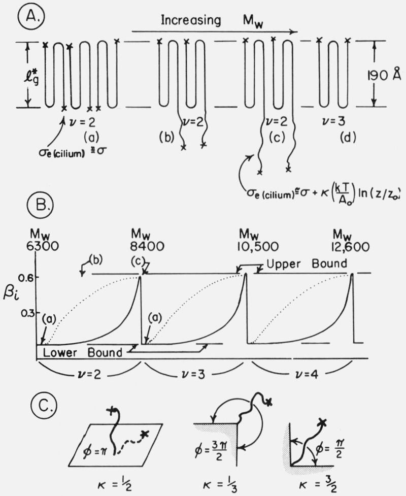
Item B calculated for case l*_g = 190 Å.

Treating the observed surface free energy of the surface nucleus (and subsequent steps) as the sum of the effects of cilia and folds we may write [3]

$${\sigma }_e={\sigma }_{e(\infty )}\left[\left(\nu +{\beta }_i\right)/(\nu +1)\right]$$ (18)

where σ_e(∞) is the limiting value of σ_e at high molecular weights corresponding to a strictly folded surface, and v the number of folds per molecule on a substrate of width l*_g. The quantity β_i is

$${\beta }_i={\sigma }_{e(\text{cilium})}/{\sigma }_{e(\infty )}$$ (19)

where σ_e(cilium) is the local contribution associated with a cilium (or chain end in the surface)to the average surface free energy. We will take σ_e(∞) to be 93 erg/cm² for preliminary calculations. This will prove to be within a few percent of the “best” value.

Specific attention is drawn to the fact that eq (18) was derived [3] on the assumption that the first chain end is situated essentially flush with the fold surface as shown schematically in figure 13A. One basic reason for making this assumption (entirely apart from its simplicity) is that it minimizes the local surface free energy associated with a molecule that is forming a nucleus on the substrate. This assumption involves the implication that the molecule to be attached has time to sample various configurations before it becomes a surface nucleus, or participates in the subsequent strip completion process, Evidence exists suggesting that molecules are physically adsorbed to some extent prior to crystallization, and crystallize after transport across the surface [1, 2]. Such a process would allow ample opportunity for the assumed configuration to occur. In practice, it is sufficient that the first chain end be associated with a quite short cilium rather than one that is always exactly flush with the fold surface.

As a useful simplification, we will assume that the width of the substrate, l*_g, is approximately constant in the region of interest. (It is apparent in table 2 that L₂ generally has a value in the range of 200±20 Å; later we shall calculate that l*_g is within the same limits.) In the case of a nearly constant substrate width, it is seen in figure 13A that as the molecular weight is increased (a) through (d) that the pendant cilium at first gets longer as the molecular weight increases [(a) through (c)]. Then as the cilium becomes as long as l*_g, a new fold appears at v+l with a short cilium, and the process repeats itself, (d). This process will cause σ_e(cilium), and hence β_i to vary in some manner (solid and dotted lines in fig. 13B) between the lower and upper bounds of β_i.

The experimental σ_e data in figure 12B exhibit rather definite upper and lower bounds. This shows that β_i in eqs (18) and (19) has a corresponding upper and lower bound. Let us now attempt on a theoretical basis to estimate the upper and lower bounds of βi. We obtain the lower bound by setting σ_e(cilium) ≅ σ = 14.2 erg/cm², which with σ_e(∞) = 93 erg/cm², gives β_i, = 0.153. This leads to

$${\sigma }_{e(\text{lower bound})}=93\{(\nu +0.153)/(\nu +1)\}.$$ (20a)

Assuming that l*_g = 190 Å, each stem has a molecular weight close to 2100. The molecular weight M at each integral v value is 2100 (v+ 1), which leads to

$${\sigma }_{e(\text{lower bound})}=93[(M-1779)/M].$$ (20b)

This function is plotted in figures 12B and 14. It is seen to give a reasonable description of the lower bound of the data from M_w ≅ 5,000 upwards.

Figure 14. σ_e as a function of molecular weight for axialites showing effects of long and short cilia as v → v + 1.

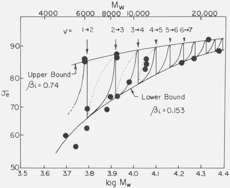
The solid and dotted lines are due to variation of β_i within a given v as shown in figure 13B.

Consider now the upper bound. We have heretofore introduced the concept that the initial surface nucleus (and subsequent molecules in the strip completion process) may exhibit a pendant cilium (fig. 13A). There is considerable independent justification for the assumption that cilia can exist in unthickened crystals. (For example, Keller and Priest have demonstrated that a substantial fraction of the end groups in polyethylene single crystals are external to the body of the crystal [36].) With this concept, we proceed by assuming that the upper bound of σ_e corresponds to a surface containing the largest cilium that can occur, which has a length closely approaching l*_g; a cilium that is any longer will fold over, giving a chain end in the surface at v+l. Lauritzen and DiMarzio [37] (LD) have devised an expression for the surface free energy contribution of a long cilium where, in its entropic wandering, configurations outside of a wedge angle ϕ are excluded (fig. 13C). Taking account of the fact that a “zero” length cilium has a surface free energy of approximately σ, the LD expression may be written

$${\sigma }_{e(cilium)}\cong \sigma +\kappa (kT/ab)\text{ln}\left(z/z_0\right)$$ (21a)

where

$$\kappa =\pi /2\varphi .$$ (21b)

In this expression z₀ is the “effective” or “statistical” segment length, which is about 6.7 for polyethylene [38], z the number of —CH₂— units in the cilium, and ab the cross-sectional area A₀ of the chain. The quantity kT/ab is 29.3 erg/cm² at T = 400 K for polyethylene. The expression is only valid for values of z/z₀ that are in excess of about 5. (It also gives the correct result σ_e(cilium)=σ for z/zo=l.) Equation (21a) is a more general case which extends the earlier calculations of DiMarzio [39] demonstrated only for the situations where ϕ = π/2 and ϕ = π.

Assuming that the cilium emanates from a plane, i.e., ϕ = π, which gives κ= 1/2, we calculate using σ = 14.2 erg/cm² and l*_g = 190 Å (z ≅ 150) in eqs (19) and (21a) that

$${\beta }_{i(\text{upper bound})}\cong \mathrm{0.642.}$$ (22)

Because of the uncertainty in ϕ, and other factors, this must be regarded as only a rough estimate. Also, the effect of the volume excluded by nearby cilia is not considered. Nevertheless, the point remains that it is reasonable that a long cilium has a high local surface free energy associated with it, which leads to a β_i that is much higher than that of a short cilium or chain end in a surface.

Using the above estimate, we may calculate

$${\sigma }_e{}_{\left(\text{upper bound}\right)}=93\left[\left(v+0.642\right)/\left(v+1\right)\right]$$ (23a)

or, using M=2100 (v+l):

$${\sigma }_e{}_{\left(\text{upper bound}\right)}=93[(M-752)/M].$$ (23b)

A plot of this function is shown in figure 12B. The agreement is such as to suggest that the surface nuclei that are associated with the high values of σ_e (e.g., 6.15, 6.15 K(R) and 8.56, 8.56 K(R)) possess long terminal cilia approximating l*_g in length. Meanwhile, it appears highly probable to us that those data points that lie near the lower bound are associated with quite short initial and terminal cilia, or initial and terminal chain ends actually in or nearly in the same plane as the folds (see fig. 13A). An analysis of the high points in ß_i = 0.74 (fig. 14).

The “best” value of σ_e(∞) is close to 90.5 erg/cm² (table 6, item C.3). The foregoing analysis could be repeated with this value instead of our original estimate of 93 erg/cm², but the change in both the theoretical and experimental estimates of β_i (upper bound) and β_i (lower bound) would be insignificant.

Sanchez and DiMarzio have developed a theory of crystallization with chain folding that deals with the variation of growth rate with molecular weight and polymer concentration [40, 41]. They employ the assumption that the initial chain end is rather long— about one-third to one-sixth of the whole molecule forms the initial cilium — in contrast to our simplified assumption that the initial chain end is practically flush with the fold surface (fig. 13A). If their assumption were to be used in the present work, a large effective value of β_i would be calculated with eq (21) for the initial cilium that would give σ_e values that greatly exceeded our calculated and experimentally determined lower bound (β_i ≅ 0.15) and which would possibly even exceed the upper bound. While we thus have good reason for holding to our particular assumption regarding the nature of the placement of the initial chain end in bulk crystallization, it must be remembered that other aspects of the treatment of Sanchez and DiMarzio confine its validity to rather dilute solution. Nevertheless, an extension or revision of their theory using the assumption that the first chain end is quite short is probably worth some consideration.

The experimental values of σ_e and β_i vary intermittently between rather definite upper and lower bounds at low molecular weights, and it is shown above that these bounds can be reasonably explained in terms of the length of the terminal cilia associated with the molecules comprising the surface nuclei and growth strip. We now ask why the values for σ_e intermittently vary between the upper and lower bounds. The explanation suggested below implies that β_i and σ_e actually alternate between their upper and lower bounds. Despite the large number of samples studied, the data are insufficient to show actual alternation over a wide range of molecular weights. However, there is some evidence for a regular variation over a restricted range of molecular weight. Accordingly, the explanation offered below for the variation of σ_e and β_i between their upper and lower bounds must be regarded as somewhat tentative.

For a given value of v, say v=2, the terminal cilium length in the model shown in figure 13A increases uniformly as the molecular weight increases. Then the cilium reaches a length of l*_g where v→ v+ 1, and the cilium length again becomes very small. This will lead β_i to alternate between the lower and upper bounds as the molecular weight increases as shown in figure 13B. We emphasize again that this holds only if J*_g does not vary strongly with molecular weight as the molecular weight changes. The details of the variation of β_i with molecular weight (increasing cilium length) with a given v is a matter of considerable uncertainty. Equation (21) suggests a situation as shown by the dotted lines in figures 13B and 14. This assumes an extremely sharp fraction. If it is arbitrarily assumed that the variation of β_i with increasing cilium length is as shown in the solid line in figure 13B, the estimates of the rather abrupt variation of σ_e with molecular weight seem appropriately predicted at v = l → v = 2 and v = 2 → v = 3, as shown in figure 14.

It is possible that the tendency for many of the experimental points that lie between v and v+l that imply a lower β_i than that given by eq (21) [dotted lines in figures 13B and 14] is a result of the existence of the distribution of molecular weight in the samples. There should be a natural tendency in the presence of a distribution for the nucleus to select out chains with short cilia (low β_i) leading to σ_e values near lower bound. Then when just the appropriate molecular weight corresponding to a long cilium is reached, the search for molecules leading to short cilia is difficult, and the system shows a high β_i and enhanced σ_e. At a slightly higher molecular weight, the long cilia folds over, and a low β_i and σ_e is rather abruptly recovered.

Our overall conclusions are as follows. The upper and lower bounds exhibited by σ_e and β_i, at low molecular weights are a result of cilium length effects in the growth nucleus. A terminal cilium in or near the fold surface is associated with a low β_i and σ_e, and a terminal cilium that approximates l*_g in length leads to a high β_i and a σ_e near the upper bound. The increase and decrease of cilium length shown in figure 13A with increasing molecular weight is probably the cause of the existence of a rather definite upper and lower bound to σ_e at low molecular weights. This model implies that β_i and σ_e should alternate in a regular way between their respective upper and lower bounds. The data are insufficient to show this in detail, but abrupt changes in β_i and σ_e occur in two regions of molecular weight that are consistent with the model. Many more good fractions — and possibly much sharperones — than were available to us would be required to obtain experimentally the shape of the β_i curve within a given v.

Attention is now drawn to the question of the constancy of l*_g, which approximation was used in the foregoing analysis. The value of the initial lamellar thickness l*_g for single crystals of polyethylene of high molecular weight can be accurately calculated as a function of undercooling with the expression [1]

$$l_g^{*}=2{\sigma }_e{T}_d^{°}/\left(\Delta h_f\right)(\Delta T)+C_2$$ (24)

where C₂ = 4.3 × 10⁻⁷ cm or 43 Å. This expression, which has a general theoretical basis, is quantitative for a thickness range of ~ 100 Å to near 200 Å for crystals formed from dilute solution [1]. We adapt this expression to the present case, and calculate l*_g for each of the fractions using σ_e from figures 12 or 14, the T°_m relevant to the fraction, and the average undercooling $\overline{\Delta T}$ used in the growth rate runs (table 3)¹⁴. The results are shown in figure 15. It is seen that l*_g is predicted to be in the range 200±20 Å from M_w ≅ 6000 upwards, which covers the cases v = 1 → 2. and all higher v. Also shown are the LAXR “L₂” data for several of the fractions. In general, these lie within the same range as the l*_g values calculated with eq (24). This confirms the validity of the assumption concerning the approximate constancy and magnitude of l*_g that was used in the calculations cited above for M_w ≥ 6000. At very low molecular weights, the low value of σ_e causes l*_g as calculated by eq (24) to fall well below 200 ±20 Å.

Figure 15. Experimental and theoretical values of the initial lamellar thickness l*_g as a function of molecular weight.

It is of interest to comment on why l*_g was so nearly constant in the particular case of polyethylene fractions of M_w ~ 6000 and higher. We may write the expression for the growth rate in the form

$$G\cong G_0\text{\hspace{0.17em}exp}\left[-U^{*}/R\left(T-T_{\infty }\right)\right]\text{\hspace{0.17em}exp}\left[-2b\sigma l_g^{*}/kT\right]$$ (25)

to a good approximation. Then if G were measured within the restricted range of ~ 10⁻⁵ cm/s to ~ 10⁻⁸ cm/s, it is easy to show that l*_g will increase by only about 10 percent or so as G goes from 10⁻⁵ cm/s to 10⁻⁸ cm/s. What happens is that l*_g increases with temperature according to eq (24) in accord with theory and experiment, but this increase for any given specimen is small compared to l*_g (or the maximum cilium length) because of the restricted temperature range allowed by the practical matter of the slowest and fastest rates that are feasible to measure.

With the analysis given in this section, it is justified to say that we have gained some insight into the factors that govern the growth rate of polyethylene from the melt from a molecular weight corresponding to but two folds per molecule (circa M_w ~ 6000) up to a molecular weight in excess of 800,000.

7. Work of Chain Folding

The “best” value of σ_e(∞) given in table 6 (item C.3) is 90.5 erg/cm². While there are various ways to estimate this quantity, this value represents a reasonable compromise and is consistent with the growth rate data within rather narrow limits. This can be used to calculate a “kinetic” value of the work of chain folding q as

$${\sigma }_{e(\infty )}(\text{kinetic})=(q/2ab)+{\sigma }_{eo}$$ (26)

where σ_e0, which is the surface free energy in the absence of any work of chain folding, may be taken as equal to σ=14.2 erg/cm² (table 6, item C.1). This leads to the estimate

$$q(\text{kinetic})=4.09\pm 0.4\text{\hspace{0.17em}kcal}/\text{mol.}$$ (27)

The corresponding estimate of q from equilibrium data on single crystals of polyethylene (i.e., σ_e(eq) = 93±9 erg/cm² from a T_m versus 1/l plot) gives with σ_e0 = 14.2 erg/cm² the value [1]

$$q\text{ (equilibrium)\hspace{0.17em}}=4.23\pm 0.4\text{\hspace{0.17em}kcal}/\text{mol.}$$ (28)

The agreement between the “kinetic” and “equilibrium” estimates of q in polyethylene is sufficient to support our particular application of nucleation theory to the problem of chain folding. The folds are kinetically formed continuously during the crystallization process, and exhibit the same properties whether their free energy of formation is measured by kinetic or thermodynamic means.

It is of interest in connection with the foregoing estimates that theoretical calculations by Corradini and co-workers using inter- and intra-potential energy functions have suggested that

$$q(\text{theoretical})=4.26\text{\hspace{0.17em}kcal}/\text{mol}$$ (29)

for (110) type folds [42]. It may be recalled that our analysis in which we find q (kinetic) = 4.09±0.4 kcal/mol is based on the assumption that (110) type folds control the growth kinetics; we also observe that the experimental value of q (equilibrium) = 4.23±0.4 kcal/mol is based on melting data on single crystals with mostly (110) folds.

Corradini and co-workers estimate a q value closeto 3.1 kcal/mol for (200) folds. The accuracy of these calculations is difficult to assess. Nevertheless, in view of the agreement attained between q(kinetic), q(equilibrium), and the q(theoretical) estimated by Corradini et al., in the case of (110) type folding, it is reasonable to assume that their theoretical estimate of q from potential energy functions for the (200) folds is basically correct. This then raises the question of why the lower energy (200) folds, known to occur in ordinary polyethylene spherulites [25], do not make themselves more apparent in the kinetics.

If two types of folds of different q were present in a given morphology, it is by no means certain that the low one would be clearly observed in kinetic measurements. Circumstances occur where both (110) and (200) type folds appear on the same overall growth front. For example, Keith [43] has shown that the overall growth front of polyethylene spherulites forming from concentrated solutions of pure hydrocarbons are serrated, with alternate and intersecting traverses of (110) and (200) folds, the latter being in the direction of overall growth, which is along the b axis of the unit cell. The polymer lamella resembles a laurel leaf with serrated edges, with the growth direction corresponding to the long axis of the leaf. The (110) folds occur at the growth tip, and at each serration. In this case — which we consider to be reasonable in a spherulitic morphology in bulk polyethylene — the kinetics of radial growth would tend to be dominated by the higher energy (110) folds until the (200) runs became quite long in comparison with the (110) runs. Possibly the presence of (200) folds is the reason that σσ_e(∞) for the coarse-grained non-banded spherulites is slightly lower than it is for the axialites (table 6). However, it must be noted again that the difference between the σσ_e(∞) in these two cases has a somewhat doubtful statistical significance. In any case it appears that (110) type folds generally dominate the kinetics of overall growth in axialites and irregular spherulites, and have the largest effect in the case of the coarse-grained non-banded spherulites.

8. Discussion

8.1. Relationship to Earlier Work: Growth Rate and Morphology

The principal previous research on the rate of growth of crystals from the melt in polyethylene appears to be that of Lindenmeyer and Holland [4]. They used five specimens ranging from M_v = 3900 to 135,000 in molecular weight. They mention the presence of banded spherulites only, whereas we found axialites over most of this molecular weight range at low undercoolings, and coarse-grained non-banded spherulites at higher undercoolings. There is no evidence of a break in log G versus T in their data, but this is explained by the relatively low growth temperatures used in their investigation. The quantitative agreement in absolute growth rates between our work and theirs is not particularly good. This can be traced in part to the fact that some of their runs were made at temperatures low enough to produce crystallization that was apparently sufficiently rapid to cause some self-heating. Also we infer from their paper that they may have used very high T₁ values which might have degraded the samples somewhat. Nevertheless, their data, when plotted as log G versus l/T(ΔT) (see their fig. 3), show changes in slope in the low molecular weight region very similar in broad aspect to that shown in our figure 8A. This implies that K_g increases and then levels off, as we found in the present research. No intermittent high and low values at low molecular weights were observed, but this may have resulted from the relatively few samples used.

It is of considerable interest to compare what we have found for polyethylene fractions with the results reported for a systematic study of TMPS fractions by Magill [44]. In this work, it was found that σσ_e rose rapidly at first and then tended to level off at high molecular weights, and Magill interpreted this as meaning that σ_e behaved with increasing molecular weight in the same manner. Moreover, Magill noted some variations of σ_e at low molecular weights (but still well within the region where folding occurs) that are strongly reminiscent of the intermittent high and low data for σ_e for polyethylene fractions near M_w = 6200 and M_w,= 8500 as seen in figures 12 and 14. In particular, one of the low TMPS fractions (M=8700) has a σ_e that is substantially higher than that of neighboring points. (Recall that in polyethylene we have tentatively attributed this type of behavior to the occasional appearance of a terminal cilium close to l*_g in length on the growth nucleus.)

Most of the data points on TMPS were taken at rather high undercoolings, corresponding, in our estimation, to regime II or mixed regime I and regime II [1]. It is therefore not surprising that Magill did not observe a regime I → regime II transition. Our analysis of the growth data, given elsewhere [1], suggests that σ_e(∞) for TMPS is 34 ± 11 erg/cm², which is in fair accord with the value σ_e(eq) = 39 erg/cm² obtained from a T_m versus 1/l plot.

Devoy and Mandelkern [45] have discussed polymers where σσ_e rises and then levels off with increasing molecular weight. Their analysis differs in a number of significant respects from that given in this work.

8.2. Regime I and Regime II in Other Polymers: Morphological Implications

Definite evidence for the existence of regime I and regime II crystallization was found for polyethylene fractions in the intermediate molecular weight range. The regime tests gave clear-cut results in this region, and the K_g values differed by a factor of about two. Also, the ratio of the pre-exponential factors was very large and of approximately the magnitude expected.

We must now raise the question as to why no such effect was seen by previous investigators for polyethylene or any other polymer crystallizing from the melt. In the case of polyethylene the answer is fairly straightforward. Few measurements, if any, were previously made at undercoolings sufficiently low to enter regime I. For example, Lindenmeyer and Holland carried out the main body of their investigations at temperatures below 127 °C, and the transition between regimes I and II occurs near or above this temperature. This same point probably accounts in part for the failure to observe the transition in other polymers — at high growth temperatures where regime I is entered, the growth rate tends to be extremely slow and the region is therefore quite inconvenient to survey from an experimental standpoint.

It has already been pointed out that the regime I → regime II transition is smeared out in polyethylene with a broad distribution of molecular weight. This is particularly clear in the case of the whole polymer SRM 1475 sample. On this basis, one might not expect to find the transition in other polymers where the distribution was broad. It will be a matter of interest to see if fractions of other polymers exhibit the transition.

It is of special interest to note that Cooper and Manley [46] have found some evidence for the existence of a regime I → regime II transition in polyethylene fractions crystallized from dilute solution. We observe that the transition, though not as well-defined in the dilute solution case as in the case of crystallization from the melt, appears to occur at approximately the same undercooling in both cases. We also observe that at a specified concentration, σσ_e as calculated with K_g = 3bσσ_eT°_d/(Δh_f)k, where T°_d is the dissolution temperature, tends to rise and then level off with increasing molecular weight when the variation of T°_d with molecular weight is taken into account (see their table 6). They find a σσ_e at high molecular weights comparable to that which we have found for melt-crystallized polyethylene.

In the case of polyethylene fractions in the low and intermediate molecular weight range, a good correlation exists between morphology and regime. Regime II kinetics could in general be identified with the existence of coarse-grained non-banded spherulites, (or spherulites with a few coarse bands at the lowest isothermal growth temperatures), and the appearance of axialites at high growth temperatures is, broadly speaking, associated with regime I kinetics. Also, the existence of irregular spherulites at high molecular weights seems to mostly involve mixed regime I and II kinetics. While these identifications seem reasonably definite for polyethylene fractions crystallized from the melt, it is not known how widely applicable the general idea of the relationship between regime and morphological characteristics really is for fractions in other polymers.

8.3. Overview

The following summarizes the basic picture of crystallization that has evolved.

The rate of crystallization of polyethylene fractions from the melt is governed by the rate of deposition of folded surface nuclei on the previously formed substrate. The nucleus is formed by a molecule (probably already associated with the substrate by physical adsorption [1]) that apparently arranges its first chain end in such a way as to keep the free energy near a minimum, i.e., the initial chain end is flush or nearly so with the fold surface. Then the rest of the molecule comes into crystallographic register with the substrate in a sequential process, leaving a dangling terminal cilium if the contour length of the molecule does not correspond to an integral multiple of the fold period l*_g. On the average, the pendant cilium does not exceed the fold period; if it is longer than l*_g a new fold is formed, and the long cilium goes down on the substrate. A sufficiently short terminal chain end has a low effective surface free energy σ_e(cilium) ≅ σ, and a long terminal cilium has a σ_e(cilium) that is proportional to the natural logarithm of the effective chain length z/z₀, giving a σ_e(cilium) value that is many times larger than σ. The value of σ_e(cilium) for a long terminal cilium of length l*_g is roughly comparable to, but probably not in excess of, σ_e. Since the average terminal cilium length is such that its local surface free energy σ_e(cilium) is less than that associated with a chain fold, the total average surface free energy (cilia plus folds) is rather low for material of low molecular weight where the fraction of cilia is rather high. As the molecular weight is increased, the fraction of folds likewise increases, and the average value of the surface free energy σ_e tends toward a limiting value, σ_e(∞).

For a given number of folds and a fixed substrate width l*_g, a surface nucleus can have either a very short cilium, one of intermediate size, or one closely approaching l*_g in length, depending on the contour length of the molecule forming the nucleus. Since the local surface free energy of a long cilium is greater than that of a short one, alternating values of σ_e are to be expected in very sharp fractions at low molecular weights as with increasing molecular weight a molecule goes through the sequence: short cilium → intermediate length cilium → cilium approaching l*_g in length → formation of additional fold with short cilium. This effect is believed on a tentative basis to be the source of the intermittent low and high values of σ_e observed at low molecular weights in the particular fractions employed in the work reported here.

The surface nucleation rate ¿, which is proportional to exp [—4bσσ_eT°_m/(Δh_f)(ΔT)kTf], leads to overall observable growth of two types. At high growth temperatures (low undercoolings) the nucleation rate is low, and each nucleus causes the completion of the substrate of length L. Then a new nucleus forms, and the process is repeated forming a lamellar crystal. In this case, regime I, the growth rate G is proportional to the nucleation rate i. At lower growth temperatures, (high undercoolings) the nucleation rate becomes quite high, and many surface nuclei are formed on the substrate. Then regime II is entered, and G is proportional to i^1/2, again with the formation of a lamellar crystal. The transition between regimes I and II is experimentally quite sharp in good fractions, and the undercooling where it occurs can be explained in terms of a value of L that is roughly 5 μm. The sharpness of the transition is fundamentally a result of the rapid change of i with undercooling.

At moderate to high molecular weight, the nucleation rate and the concomitant overall growth rate are not strongly dependent on changes of viscosity of the melt from which the various crystalline bodies are formed. Also, the nucleation rate, as measured by σσ_e, appearsto be nearly independent of such factors as the presence of interlamellar links at high molecular weights. The absolute value of the pre-exponential for regime I is much greater than that for regime II, principally because that for regime I contains the factor L, whereas that for regime II does not.

The observed value of the initial lamellar thickness l*_g is in general close to that predicted from the under-cooling and the σ_e relevant to the molecular weight under consideration. Because the growth rate G is related to l*_g according to G ∝ exp (−2bσl*_g/kT), and because the experimental range of G is limited, l*_g is itself restricted in polyethylene crystallizing isothermally from the melt to a rather narrow range close to 200 Å.

The work of chain folding q can be deduced from strictly kinetic measurements. The value so obtained is in close agreement with that from equilibrium measurements on polyethylene single crystals, and with certain theoretical calculations. There appear to be no inconsistencies of an energetic character in the picture of crystallization presented here.

The authors thank Esmund Drott of the Monsanto Chemical Company for supplying some of the fractions, and J.J. Weeks, Jr., for his considerable assistance in carrying out the WAXR and LAXR measurements. We also gratefully acknowledge a number of discussions with E. A. DiMarzio and F. Khoury. We are indebted to H. D. Keith for pointing out the significance of his work on crystallization of polyethylene from pure hydrocarbons, and for a number of timely discussions.