Segregation through the multiscalar lens

Significance

We develop a method of measuring segregation which captures the multidimensional nature of mixing in metropolitan areas. The use of trajectory convergence analysis provides a flexible way for capturing change across all scales from small spatial units and how the rate of convergence to the citywide average modifies over space. Thus, the method provides an analysis of how far, in spatial terms, any individual or neighborhood is from the citywide multigroup distribution. We use this method to investigate ethnic mixing in the Southern California metropolitan region. The results illustrate excellent visual measures of the patterns of mixing across urban space, and the graphical trajectories reveal the spatial speed at which the process of convergence takes place.

Abstract

We introduce a mathematical framework that allows one to carry out multiscalar and multigroup spatial exploratory analysis across urban regions. By producing coefficients that integrate information across all scales and that are normalized with respect to theoretical maximally segregated configurations, this framework provides a practical and powerful tool for the comparative empirical analysis of urban segregation. We illustrate our method with a study of ethnic mixing in the Los Angeles metropolitan area.

Indices of spatial dissimilarities continue to be at the center of studies of ethnic (and other forms of) segregation in large cities (1–13). However, single-number indices as well as single-scale indices cannot capture the complexity of spatial patterns that arise in actual cities. Only recently, this has led to the exploration of multiscalar approaches (14–23), including multidimensional, matrix indices (24). We present in this paper a framework that allows one to carry out fully multiscalar analyses of spatial dissimilarities and to define multiscalar null models. This framework provides powerful visual representations of segregation phenomena, and it has the capacity to characterize segregation phenomena in a fashion very similar to what may be perceived in actuality.

Our starting point is indeed the common experience that any individual may make of segregation on multiple scales. Consider a city, the population of which comprises $k$ groups. Imagine that an individual explores the city from her home, looking first at her direct neighbors and then at the building next door, and so on, in an ever-expanding visual scale. She will gradually meet the whole city, but at every step, the proportions of the groups in the population that she has encountered so far produce a sequence that yields detailed information on the starting point, in multiscalar relationship with the whole city. We show in Methods how this information may be extracted and analyzed mathematically. In Ethnic Segregation in Los Angeles, we illustrate our method by conducting a study on ethnic mixing in the Los Angeles area.

Methods

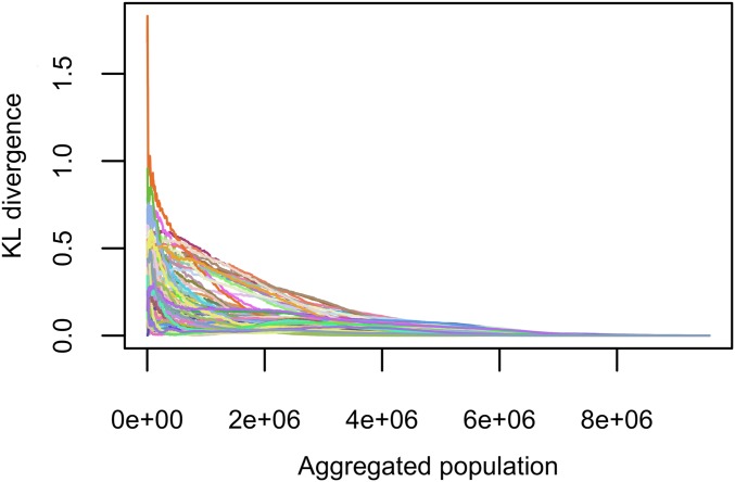
We formalize the idea of exploring a city at every scale, from every possible starting point. This is a generalization of a method introduced in ref. 23: Given a starting point and an aggregation procedure (e.g., a nearest-neighbor rule), one may sequentially aggregate all individuals in the city. The aggregated sequence then encodes the order in which someone, starting from that particular point, would encounter the city’s inhabitants.* If to each individual in the city one associates a characteristic of interest (ethnicity, income, …), then one may also compute the statistical distribution of that same characteristic at every “instant”—in terms of population—of the aggregated sequence. At the first point of the sequence, one has the distribution within the starting spatial unit, whereas at the final point, one has the distribution of the entire city, since all individuals have been aggregated. Instead of considering sequences of statistical distributions computed on ever-larger aggregated populations, one may measure the difference between these and that of the reference population in the entire city. Hence, for each starting point, we shall obtain a dissimilarity trajectory that eventually converges to zero. Furthermore, the trajectories will vary from one starting point to another, reflecting the fact that individuals have different experiences of the city according to where they live: The way each trajectory converges to 0 encapsulates, for each starting point, all information at every scale, from the most local one to the metropolitan one. In this sense, the set of trajectories obtained starting from all points constitutes a fingerprint of the city for the characteristic under consideration (see Fig. 2).

Fig. 2.

Trajectories for KL divergence, starting from some (10%) of the tracts in the Los Angeles area. Abscissae are expressed in terms of the aggregated population around the starting point. All trajectories converge to 0, but some do so quickly, while others reach 0 only at much larger scales.

We are interested here in a particular type of distributions, namely, multinomial. That is, we suppose we have $k$ groups in the population, $A_1,A_2,A_3,\dots ,A_k$. To measure the difference between distributions, we use the Kullback–Leibler (KL) divergence.

KL Trajectories.

The KL divergence (25) between two multinomial distributions $\left(q_1,\dots ,q_k\right)$, $\left(r_1,\dots ,r_k\right)$ is defined as

$$d_{\mathrm{K}\mathrm{L}}\left(q\mid r\right)=\sum _{i=1}^k{q}_i\ln \frac{q_i}{r_i},$$ [1]

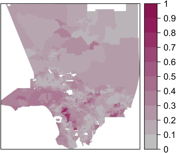
with the convention $0\ln 0=0$. The KL divergence quantifies the nonlinear variation in entropy incurred when substituting distribution $q$ for the reference one, $r$. Note that computing the KL divergence for each unit and then averaging over all units (weighting each unit by its size) leads to the $H$ index (8)—which is the so-called KL information (26). One may plot the value of the KL divergence for each spatial unit in a region. See, for instance, Fig. 1, where we have done so for the Los Angeles area (at the tract level).

Fig. 1.

A map of the Los Angeles area with tracts colored according to the KL divergence between their ethnic composition and that of the whole region. Darker colors represent greater divergence. Values have been normalized by their maximum, so that they scale from 0 to 1. (Four ethnic groups are considered: Whites, Hispanics, Asians, and Blacks. Data are from the 2010 US Census.)

Building upon the idea of trajectories previously introduced, we define, for every starting point in the city, its KL trajectory. This is obtained by computing the KL divergence between the distribution on the aggregated population and the reference population. As the aggregation process relies on a spatial nearest-neighbor rule, a KL trajectory is moving from the most local scale through to the whole region. It represents at each step the divergence between the distribution in the population met so far and the distribution in the full region. Mathematically, if $q^{i,1:u}$ is the statistical distribution of the population in the $u$ closest units to $i$, the KL trajectory associated to unit $i$ is simply the sequence

$$d_{KL}\left(\left.q^{i,1:u}\right|\hspace{0.17em}r\right),\hspace{1em}1\le u\le U,$$ [2]

where $r$ is the distribution in the full population and $U$ is the number of spatial units in the city.

By construction, every KL trajectory eventually converges to 0 (Fig. 2). However, trajectories differ widely from one starting point to another. Some converge quickly to 0, corresponding to areas where even relatively small aggregates present a reasonably good picture of the whole city. Other trajectories, on the contrary, converge very slowly to 0, corresponding to areas where segregation effects build up across scale and accumulate far beyond the local, tract level.

Focal Distances.

We are interested in quantifying the convergence of each trajectory, and the speed at which this occurs, as a mark of segregation of the corresponding starting point. If one fixes a convergence threshold $\delta$, it is then possible to compute, for each trajectory, the instant when it enters (and remains thereafter) in the interval $\left[0,\delta \right]$. This instant is the size of the population that one needs to aggregate, for a given starting point, to have a distribution of groups that remains within KL divergence $\delta$ of the reference distribution. In other terms, this is, for a given starting point, how far one needs to go in the aggregation process to see (with precision $\delta$) the city’s population as it is in its globality—the distance one needs to cover to get a relatively clear picture of the city. We call this convergence size the focal distance. Formally, the focal distance at point $i$, with precision $\delta$, is defined as

$$f_i\left(\delta \right)=\underset{u}{inf}\left\{n_{i,1:u}\hspace{0.17em}\hspace{0.17em}|\hspace{0.17em}\forall ũ\ge u,d_{KL}\left(\left.q^{i,1:ũ}\right|\hspace{0.17em}r\right)\le \delta \right\},$$ [3]

where $n_{i,1:u}$ is the size of the population in the $u$ closest units to unit $i$.

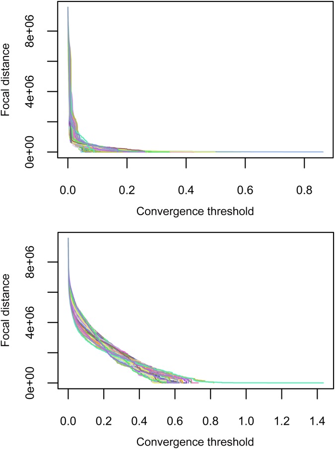
There is, of course, some arbitrariness in the choice of the convergence threshold $\delta$, but this may be circumvented by considering all its possible values. For any starting point $i$ and for $\delta =0$, convergence occurs only at the very end of the KL trajectory, so that $f_i\left(\delta \right)=N$ ($N$ is the total population). When $\delta$ is large (typically, larger than the maximum of the KL trajectory), convergence occurs immediately so that $f_i\left(\delta \right)=0$. One may then plot the variation of $f_i\left(\delta \right)$ as $\delta$ increases (Fig. 3). The higher the curve representing $f_i\left(\delta \right)$, the longer the focal distances for $i$, even at large values of $\delta$ (i.e., when convergence is easier). This helps identifying points in a city where spatial dissimilarities accumulate on multiple scales to create veritable “hotspots” of segregation. From these points, what one perceives of the city is very much altered, even on large scales, compared with what the city looks like in actuality. We formalize this concept into what we term distortion coefficients.

Fig. 3.

Focal distance curves, starting from some of the tracts in the Los Angeles area. Ordinates are focal distances expressed in terms of the aggregated population around the starting point. They represent aggregation sizes $f_i\left(\delta \right)$ at which the corresponding KL trajectories (Fig. 2) converge, for each value of the convergence threshold $\delta$. We give exemplars of two types of behavior. (Upper) Sharply decreasing curves correspond to points with short focal distances, even for small values of $\delta$. (Lower) Slower-decreasing curves correspond to points with long focal distances, even for larger values of $\delta$. The distortion coefficient at a given point in the city is then defined (Eq. 4) to be proportional to the area under the corresponding focal distance curve: The higher the curve, the larger the coefficient.

Distortion Coefficients.

We have defined for each point $i$ in the city a trajectory of focal distances $f_i\left(\delta \right)$ with $0\le \delta \le {\delta }_{i,max}$, where ${\delta }_{i,max}$ is the maximum value of the KL trajectory associated to unit $i$. Summing up focal distances $f_i\left(\delta \right)$ for all $\delta$ gives a measure of how distorted the perception of the city is, from point $i$. Formally, we are simply integrating the focal distance curves—that is, we define the distortion coefficient of unit $i$ as

$${\mathrm{\Delta }}_i={\int }_0^{{\delta }_{i,max}}\hspace{0.17em}{f}_i\left(\delta \right)\hspace{0.17em}d\delta .$$ [4]

To enable comparisons from one variable to another, or from one city to another, distortion coefficients should be independent of the size of the city and also of the average distribution in the city. With this in mind, we compute the normalized distortion coefficients ${\tilde{\mathrm{\Delta }}}_i={\mathrm{\Delta }}_i/\mathcal{N}$, where $\mathcal{N}$ is a normalizing constant. In practice, $\mathcal{N}$ is chosen as the maximum distortion coefficient in a theoretical extreme case of segregation. Theoretically, the maximal-segregation distortion coefficient is achieved when sorting the $k$ groups into $k$ ghettos, ordered by sizes, and then computing the coefficient for the most isolated person in the smallest group. This person would first meet all of the individuals of his own group, then all those of the second-most infrequent group, and so on, until having seen the entire population of the city. The normalized distortion coefficients ${\tilde{\mathrm{\Delta }}}_i$ take values between 0 and 1 and express the levels of distortion as a fraction of the perspective one has from the theoretical maximally segregated unit (for a given population size and for given group proportions).

To apprehend the meaning of the distortion coefficients, we generate several simple, synthetic configurations. A complete description of these experimental results is provided in SI Appendix. It shows how distortion coefficients integrate information across all scales and how this method captures hotspots of multiscalar segregation, as well as fine details of how multiscalar segregation varies across space, from points with low distortion to points with high distortion.

Ethnic Segregation in Los Angeles

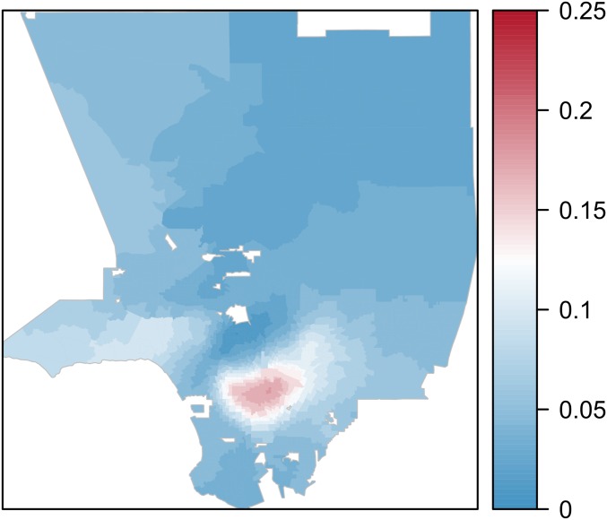
As an example, we studied the ethnic distribution in Los Angeles. We worked with 2010 US Census data and analyzed the four largest groups: Whites, Hispanics, Asians, and Blacks. For each tract in the city, the KL divergence between the multigroup distribution inside the tract and the multigroup distribution in the whole city is shown in Fig. 1. We then built the full set of KL trajectories^† (Fig. 2) and derived the corresponding focal distance curves (Fig. 3). Integrating these curves as in Eq. 4 and normalizing according to the equivalent completely segregated four-group population, we obtained the distortion coefficients for each tract, as shown in Fig. 4.

Fig. 4.

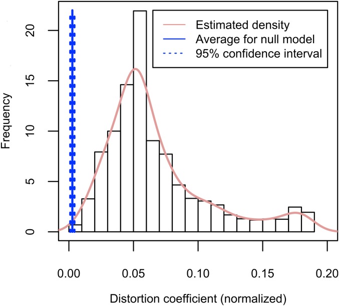
Histogram and estimated density (pink solid line) of normalized distortion coefficients in Los Angeles area. The solid blue vertical line corresponds to the average value of distortion coefficients in a null model obtained by random (spatial) permutations. The dashed line indicates a 95% confidence interval around the average in the null model.

First, let us note the order of magnitude of the distortion coefficients. These reach 0.15–0.20—that is, 15–20% of the maximal value one would obtain by completely separating the four groups into four “ghettos.” For comparison, a similar study carried out on different groups in large European cities led to values of only half a percent or a few percent (27). We may thus conclude that ethnic segregation in Los Angeles reaches moderately high levels across mesoscopic and macroscopic scales, not just at the tract level. This conclusion should, however, be considered with caution, since we still need to apply our method to other real data, to get a full perspective of what a highly segregated city should provide as distortion coefficients.

Second, the frequency distribution is particularly informative about spatial heterogeneity. Indeed, if the distribution is narrow and highly peaked at its average, then there is a high level of spatial homogeneity in the city. On the contrary, a broad distribution signals spatial heterogeneity, with multiscalar perceptions of the city varying greatly from one area to another. Frequency distributions may also exhibit more complex features, such as bimodality, suggesting the existence of subsets of segregated areas. In our case, the distribution is markedly skewed, with its peak at 6% of the theoretical maximally segregated value and a secondary mode close to the 20% mark.

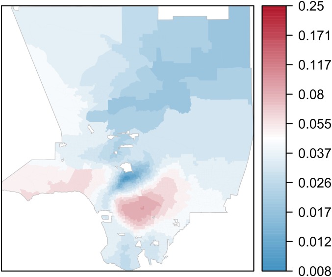
Note that finer details and fluctuations of distortion coefficients may be examined by switching to a logarithmic scale, as shown in Fig. 6. The logged representation is particularly interesting when distortion coefficients have a heavy-tailed distribution and span several orders of magnitude. While a linear scale highlights the tail of the distribution and the atypical, highly distorted units, it flattens the rest of the values, for which a logged map provides a better insight. Here, this allows us to access the secondary structure of multiscalar segregation in Los Angeles, with areas like Malibu in the west exhibiting notable levels. We also note that the tracts with the highest distortion and the ones with the lowest distortion appear to both be tightly grouped in different areas: There is a distinct group of contiguous darker blue tracts and a distinct group of contiguous darker red tracts. This is another sign of the level of spatial effects in ethnic segregation in Los Angeles.

Fig. 6.

Same as Fig. 5 but with a logarithmic color scale, allowing one to see finer details in the variation of distortion coefficients across space.

Furthermore, one may perform empirical statistical tests and check how much the given city configuration differs from a completely random one. The distribution under the null hypothesis may be easily generated by performing a large number of random permutations and then computing the associated distortion coefficients, their mean value, and a 95% confidence interval around it. According to Fig. 4, all distortion coefficients are greater than the right limit of the confidence interval for the null model, which means that the hypothesis of a completely random distribution of the four communities in Los Angeles is rejected. There is a clustered structure in the data, which means there is segregation, and the maps in Figs. 5 and 6 allow one to identify the most segregated and the most integrated areas.

Fig. 5.

A map of the Los Angeles area with tracts colored according to their distortion coefficients for the ethnic composition of the population.

Conclusion and Perspectives

The method that we have introduced in this paper offers powerful analytical and visual tools to study multigroup segregation in large urban areas.

We have shown here only a few of its capacities. Defining focal distances and distortion coefficients from the convergence of KL trajectories, we have focused on only one type of information that may be extracted from these trajectories. Indeed, other scales of interest may be obtained. Think, for instance, of the scale at which a given KL trajectory attains its maximum—this is the scale of the bespoke neighborhood that is maximally different from the city. On a more theoretical side, we note that a null model may be defined as was done in Ethnic Segregation in Los Angeles: by simply considering random permutations. Establishing the theoretical properties of this null model is not straightforward, as the trajectories obtained when moving from distributions to KL divergence are not readily modeled. In a simpler framework (23), when working with single-group proportions, one may approximate the corresponding trajectories by generalized Brownian bridges (28, 29) and transform the problem into a first-passage one for Brownian motion (30). The general version presented here does not seem amenable to the same techniques and poses an interesting mathematical challenge for future research.

Finally, we believe that this method may open new perspectives on the mechanisms driving segregation, in a well-formalized mathematical framework. Indeed, this technique can be further combined either with theoretical model-based simulations or with a broader empirical context (multiple cities, variables, or time instants), and thus further contribute into a fine understanding of segregation, of how it changes in time or across space, how microscopic and/or macroscopic interventions on the dynamics or on the spatial distribution may lead to significant changes in the trajectories and in the distortion coefficients, where these changes are the most prominent, and how they propagate over space.

References

- 1.Cowgill D. O., Cowgill M. S., An index of segregation based on block statistics. Am. Sociol. Rev. 16, 825–831 (1951). [Google Scholar]
- 2.Duncan O. D., Duncan B., A methodological analysis of segregation indexes. Am. Sociol. Rev. 20, 210–217 (1955). [Google Scholar]
- 3.Farley R., Taeuber K. E., Population trends and residential segregation since 1960. Science 159, 953–956 (1968). [DOI] [PubMed] [Google Scholar]
- 4.Cortese C. F., Falk R. F., Cohen J. K., Further considerations on the methodological analysis of segregation indices. Am. Sociol. Rev. 41, 630–637, (1976). [Google Scholar]
- 5.White M. J., The measurement of spatial segregation. Am. J. Sociol. 88, 1008–1018 (1983). [Google Scholar]
- 6.James D. R., Taeuber K. E., Measures of segregation. Sociol. Methodol. 15, 1–32 (1985). [Google Scholar]
- 7.Massey D. S., Denton N. A., The dimensions of residential segregation. Soc. Forces 67, 281–315 (1988). [Google Scholar]
- 8.Reardon S. F., Firebaugh G., Measures of multigroup segregation. Sociol. Methodol. 32, 33–67 (2002). [Google Scholar]
- 9.Brown L. A., Chung S.-Y., Spatial segregation, segregation indices and the geographical perspective. Popul. Space Place 12, 125–143 (2006). [Google Scholar]
- 10.Feitosa F. F., Camara G., Monteiro A. M. V., Koschitzki T., Silva M. P. S., Global and local spatial indices of urban segregation. Int. J. Geograph. Inf. Sci. 21, 299–323 (2007). [Google Scholar]
- 11.Fossett M., New Methods for Measuring and Analyzing Segregation (Springer Series on Demographic Methods and Population Analysis, Springer, New York, 2017), Vol. 42. [Google Scholar]
- 12.Olteanu M., Hazan A., Cottrell M., Randon-Furling J.. Multidimensional urban segregation - toward a neural network measure. arXiv:1705.03213 (9 May 2017).
- 13.Harris R., Johnston R., Measuring and modelling segregation–new concepts, new methods and new data. Environ. Plann. B Urban Anal. City Sci. 45, 999–1002 (2018). [Google Scholar]
- 14.Leckie G., Pillinger R., Jones K., Goldstein H., Multilevel modeling of social segregation. J. Educ. Behav. Stat. 37, 3–30 (2012). [Google Scholar]
- 15.Östh J., Clark W. A. V., Malmberg B., Measuring the scale of segregation using k-nearest neighbor aggregates. Geograph. Anal. 47, 34–49 (2015). [Google Scholar]
- 16.Louf R., Barthelemy M., Patterns of residential segregation. PLoS One 11, e0157476 (2016). [DOI] [PMC free article] [PubMed] [Google Scholar]
- 17.Clark W. A. V., Andersson E., Östh J., Malmberg B., A multiscalar analysis of neighborhood composition in Los Angeles, 2000–2010: A location-based approach to segregation and diversity. Ann. Assoc. Am. Geogr. 105, 1260–1284 (2015). [Google Scholar]
- 18.Jones K., Johnston R., Manley D., Owen D., Charlton C., Ethnic residential segregation: A multilevel, multigroup, multiscale approach exemplified by London in 2011. Demography 52, 1995–2019 (2015). [DOI] [PMC free article] [PubMed] [Google Scholar]
- 19.Manley D., Johnston R., Jones K., Owen D., Macro-, meso-and microscale segregation: Modeling changing ethnic residential patterns in Auckland, New Zealand, 2001–2013. Ann. Assoc. Am. Geogr. 105, 951–967 (2015). [Google Scholar]
- 20.Leckie G., Goldstein H., A multilevel modelling approach to measuring changing patterns of ethnic composition and segregation among London secondary schools, 2001–2010. J. R. Stat. Soc. Ser. A 178, 405–424 (2015). [Google Scholar]
- 21.Harris R., Owen D., Implementing a multilevel index of dissimilarity in R with a case study of the changing scales of residential ethnic segregation in England and Wales. Environ. Plann. B Urban Anal. City Sci. 45, 1003–1021 (2017). [Google Scholar]
- 22.Adrestani B. M., O’Sullivan D., Davis P., A multi-scaled agent-based model of residential segregation applied to a real metropolitan area. Comput. Environ. Urban Syst. 69, 1–16 (2017). [Google Scholar]
- 23.Randon-Furling J., Olteanu M., Lucquiaud A., From urban segregation to spatial structure detection. Environ. Plann. B Urban Analytics. City Sci., 10.1177/2399808318797129 (2018). [Google Scholar]
- 24.Ballester C., Vorsatz M., Random walk-based segregation measures. Rev. Econ. Stat. 96, 383–401 (2014). [Google Scholar]
- 25.Kullback S., Leibler R. A., On information and sufficiency. Ann. Math. Stat. 22, 79–86 (1951). [Google Scholar]
- 26.Chodrow P. S., Structure and information in spatial segregation. Proc. Natl. Acad. Sci. U.S.A. 114, 11591–11596 (2017). [DOI] [PMC free article] [PubMed] [Google Scholar]
- 27.Clark W., Olteanu M., Randon-Furling J., “Segregation, focal distances & neighbourhood scales for EU and non-EU migrants in European cities” in D4I Final Workshop (EU Joint Research Center, Brussels, Belgium, 2018). [Google Scholar]
- 28.Rosén B., Limit theorems for sampling from finite populations. Arkiv Matematik 5, 383–424 (1964). [Google Scholar]
- 29.Sen P. K., Finite population sampling and weak convergence to a Brownian bridge. Sankhyā Indian J Stat Ser A 34, 85–90 (1972). [Google Scholar]
- 30.Salminen P., Yor M., On hitting times of affine boundaries by reflecting Brownian motion and Bessel processes. Periodica Mathematica Hungarica 62, 75–101 (2011). [Google Scholar]
Associated Data
This section collects any data citations, data availability statements, or supplementary materials included in this article.